F3 Design of Control System for an Autonomous Racecar - Czech Technical University in Prague - wiki
←
→
Page content transcription
If your browser does not render page correctly, please read the page content below

Bachelor Project

                   Czech
                   Technical
                   University
                   in Prague
                   Faculty of Electrical Engineering
F3                 Department of Control Engineering

Design of Control System for an
Autonomous Racecar

Marek Boháč

Supervisor: doc. Ing. Martin Hromčík, Ph.D.
August 2020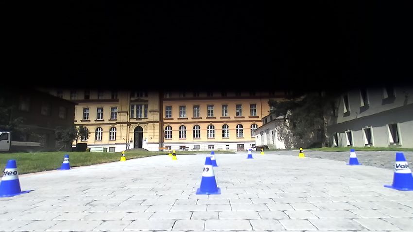
ii
BACHELOR‘S THESIS ASSIGNMENT

I. Personal and study details

  Student's name:                  Boháč Marek                                                           Personal ID number:                465967
  Faculty / Institute:             Faculty of Electrical Engineering
  Department / Institute:             Department of Control Engineering
  Study program:                   Cybernetics and Robotics

II. Bachelor’s thesis details
  Bachelor’s thesis title in English:
   Design of a Control System for an Autonomous Racecar

  Bachelor’s thesis title in Czech:
   Návrh řídícího systému autonomního závodního vozidla

  Guidelines:
   The goal is to develop new functionalities for the upcoming auton omous racing car of the eForce team of the FEE CVUT,
   related to trajectory planning and vehicle control. Specific tasks follow below.
   1) Create a mathematical model capturing key features of the kinematics and dynamics of racecar.
   2) Create a simulation environment for design and verification of the control system.
   3) Design a control system for longitudinal and lateral trajectory tracking.
   4) Implement the control system on the racecar operating system.
   5)Verify the controller experimentally.

  Bibliography / sources:
   [1] Dieter Schramm, Manfred Hiller, Roberto Bardini – Vehicle Dynamics – Duisburg 2014
   [2] Hans B. Pacejka - Tire and Vehicle Dynamics – The Netherlands 2012
   [3] Robert Bosch GmbH - Bosch automotive handbook - Plochingen, Germany : Robet Bosch GmbH ; Cambridge, Mass.
   : Bentley Publishers
   [4] Franklin, Gene F.; Powell, J. David; Emami-Naeini, Abbas, Feedback Control of Dynamic Systems, Global Edition,
   Pearson Education Limited, 2019, ISBN: 9781292274522

  Name and workplace of bachelor’s thesis supervisor:
   doc. Ing. Martin Hromčík, Ph.D.,                   Department of Control Engineering, FEE

  Name and workplace of second bachelor’s thesis supervisor or consultant:

   Date of bachelor’s thesis assignment: 31.01.2020                              Deadline for bachelor thesis submission: 14.08.2020

   Assignment valid until:
   by the end of winter semester 2021/2022

 ___________________________                          ___________________________                             ___________________________
     doc. Ing. Martin Hromčík, Ph.D.                         prof. Ing. Michael Šebek, DrSc.                           prof. Mgr. Petr Páta, Ph.D.
             Supervisor’s signature                              Head of department’s signature                                Dean’s signature

III. Assignment receipt
   The student acknowledges that the bachelor’s thesis is an individual work. The student must produce his thesis without the assistance of others,
   with the exception of provided consultations. Within the bachelor’s thesis, the author must state the names of consultants and include a list of references.

                               .
                         Date of assignment receipt                                                       Student’s signature

CVUT-CZ-ZBP-2015.1                                                                                           © ČVUT v Praze, Design: ČVUT v Praze, VIC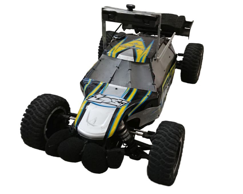
iv
Acknowledgements                         Declaration
Firstly, I would like to express my sin-          I declare that this work is all my own work
cere gratitude to my supervisor, doc. Ing.        and I have cited all sources I have used in
Martin Hromčík, Ph.D., for his advice             the bibliography.
while writing this thesis. Special thanks
                                                    Prague, August 13, 2020
belong to Ing. Jan Čech, Ph.D. for his
work for eForce Driverless as Faculty Ad-
visor. Without his advice and guidance
of the team, this thesis would not be pos-
sible. Also, my thanks go to Ing. Tomáš
Haniš, Ph.D. for initial guidance on the            Prohlašuji, že jsem předloženou práci
topic and his advice and help with adapt-         vypracoval samostatně a že jsem uvedl
ing car for RC car as the last step of this       veškerou použitou literaturu.
thesis.                                             V Praze, 13. srpna 2020
   Secondly, I would like to express my
gratitude to all my previous lecturers and
the Czech Technical University itself for
helping me gain invaluable academic and
practical experience. Last but not least, I
would like to thank the eForce Driverless
team for their hard work and collabora-
tion with me on this project.

                                              v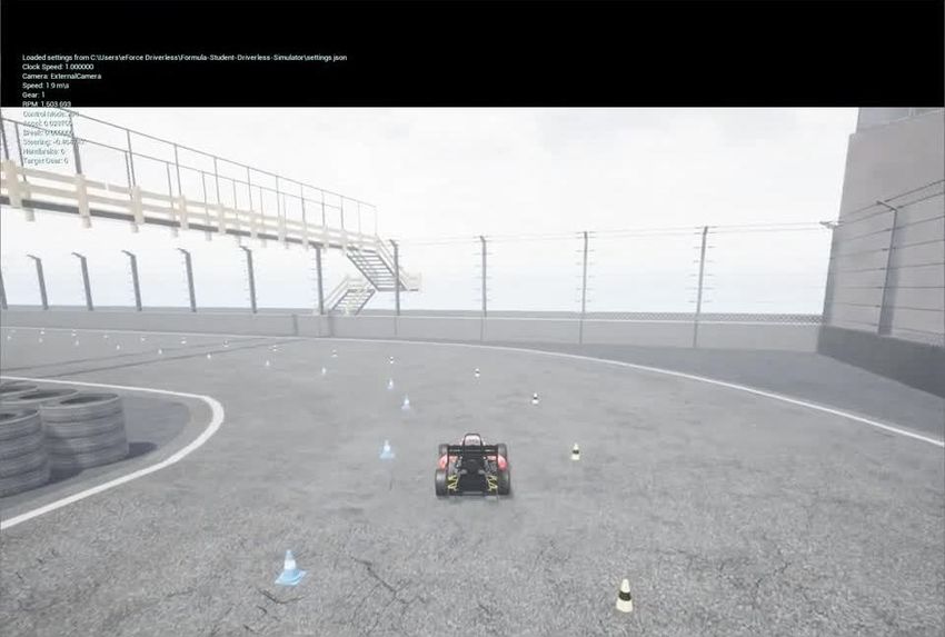
Abstract                Abstract
This thesis describes the design, develop-          V této práci se zabývám popisem návrhu,
ment, and implementation of the first au-           vývoje a implementace řídícho systému
tonomous racecar of team eForce Driver-             pro první autonomní závodní formuli
less for Formula Student competition. It            týmu eForce Driverless pro soutěž For-
is mainly focused on motion planning algo-          mula Student. Práce se zaměřuje ze-
rithms and trajectory tracking algorithms           jména na plánování pohybu, řízení vůči
and related topics such as vehicle dynam-           planované trajektorii a s tím související
ics, but it describes other systems as well.        témata jako je jízdní dynamika vozidel,
The motion planning algorithm consists              nicméně popisuje i jiné části systému.
of a path planning algorithm and a speed            Plánování pohybu spočívá v nalezení
reference generator. Trajectory tracking            cesty a následném vygenerování reference
uses Stanley control laws for lateral con-          rychlosti pro každý bod. Podélné řízení
trol and PI regulator for longitudinal con-         je poté zajištěno pomocí PI regulátoru
trol. As part of the thesis, the simulation         a příčné řízení zajišťuje implementovaný
environment was designed as well. The               řídící zákon vyvinutý na Stanfordské uni-
solution designed in this thesis was then           verzitě pro DARPA Challenge a auto poj-
used in Formula Student Online competi-             menované Stanley.
tion and implemented on a smaller plat-
form than the actual racecar to safely test         Keywords: autonomní vozidlo,
its behavior.                                       autonomní závodění, sledování
                                                    trajektorie, plánování pohybu, dynamika
Keywords: autonomous vehicle,                       vozidla, příčné řízení, podélné řízení,
autonomous racing, trajectory tracking,             formula student, formula student
motion planning, vehicle dynamics,                  driverless
lateral control, longitudinal control,
formula student, formula student                    Title translation: Návrh řídícího
driverless                                          systému autonomního závodního vozidla

Supervisor:   doc. Ing. Martin Hromčík,
Ph.D.

                                               vi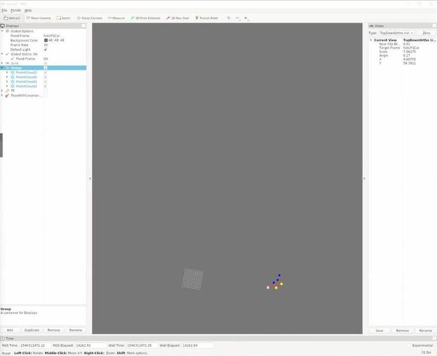
Contents
1 Introduction                                             1         10 Results                   41
1.1 Platforms . . . . . . . . . . . . . . . . . . . . .    1         11 Conclusions               43
 1.1.1 DV.01 . . . . . . . . . . . . . . . . . . . . .     2
 1.1.2 RC car . . . . . . . . . . . . . . . . . . . .      3         Acronyms                     45
1.2 Formula Student Driverless                                       Bibliography                 47
 Challenges . . . . . . . . . . . . . . . . . . . . . .    3         A DV.01 car parameters       49
2 Objectives                                               7         B ROS Simulator Parameters   51
3 Vehicle dynamics                                         9         C FSDS Parameters            53
3.1 Nonlinear single-track model . . . .                   9
3.2 Tire modeling . . . . . . . . . . . . . . . .         11         D RC Car Experiments         55
3.3 Friction circle . . . . . . . . . . . . . . . .       12         E Content of the CD          57
3.4 Model verification . . . . . . . . . . . .            13
4 Motion Planning                                         15
4.1 Path planning . . . . . . . . . . . . . . . .         16
4.2 Speed reference generator . . . . . .                 18
4.3 Simulation scenarios . . . . . . . . . .              19
5 Trajectory Tracking                             21
5.1 Lateral control . . . . . . . . . . . . . . . 21
5.2 Longitudinal control . . . . . . . . . . 22
6 System architecture                                     25
7 ROS based simulator                                     27
7.1 Steering simulation . . . . . . . . . . .             27
7.2 Vision simulation . . . . . . . . . . . . .           27
7.3 Vehicle simulation . . . . . . . . . . . .            28
7.4 Experiment with track . . . . . . . .                 29
8 Formula Student Driverless
Simulator                                               33
8.1 System adaptation . . . . . . . . . . . . 33
8.2 Results . . . . . . . . . . . . . . . . . . . . . . 35
9 Radio-controlled Car                                  37
9.1 System adaptation . . . . . . . . . . . . 37
 9.1.1 Cone detection . . . . . . . . . . . . 37
 9.1.2 Motion planning and trajectory
   tracking . . . . . . . . . . . . . . . . . . . . . . 38
9.2 Experiments . . . . . . . . . . . . . . . . . 39

                                                               vii
Figures Tables
1.1 FSE.07 car being rebuilt into 1.1 DV.01 hardware . . . . . . . . . . . . . . . 4
DV.01 [1] . . . . . . . . . . . . . . . . . . . . . . . 2 1.2 RC car hardware . . . . . . . . . . . . . . 5
1.2 Sensors placement - Top view 1, 2 -
Realsense; 3 - OS-64; 4 - ZED . . . . . 3 A.1 DV.01 model parameters . . . . . . 49
1.3 Adapted Radio-controlled (RC) car A.2 DV.01 drivetrain limitation . . . . 49
Losi Desert Buggy [2] . . . . . . . . . . . . 5 A.3 DV.01 tire parameters . . . . . . . . 50
3.1 Single track model coordinates . 10 B.1 ROS simulator parameters for
3.2 Tire model . . . . . . . . . . . . . . . . . . . 10 trajectory tracking and motion
3.3 Friction ellipse for normalized planning . . . . . . . . . . . . . . . . . . . . . . . 51
forces . . . . . . . . . . . . . . . . . . . . . . . . . 12 B.2 Noise standard deviations used in
3.4 Car position with respect to global simulation . . . . . . . . . . . . . . . . . . . . . 52
coordinates . . . . . . . . . . . . . . . . . . . . 13
C.1 FSDS parameters for trajectory
3.5 Torque command for each wheel
tracking and motion planning . . . . 53
and velocity response . . . . . . . . . . . . 14
3.6 Steering step command and yaw D.1 World-image correspondences . . 55
rate response . . . . . . . . . . . . . . . . . . . 14
E.1 CD Content . . . . . . . . . . . . . . . . . 57
4.1 Motion planning algortihm results
under different conditions . . . . . . . . 20
6.1 Base system architecture as used in
DV.01 . . . . . . . . . . . . . . . . . . . . . . . . . 26
7.1 ROS based simulator high-level
architecture . . . . . . . . . . . . . . . . . . . . 28
7.2 Steering simulation . . . . . . . . . . . 29
7.3 Autocross track and logged
position of the car . . . . . . . . . . . . . . 30
7.4 Car speed and torque command 31
7.5 Car steering angle and command 31
8.1 Formula Student Driverless
Simulator (FSDS) high-level
architecture . . . . . . . . . . . . . . . . . . . . 34
8.2 FSDS simulator . . . . . . . . . . . . . . 35
8.3 Rviz visualization . . . . . . . . . . . . . 36
9.1 OpenLabeling open-source labeler 38
9.2 Setup and picture used to obtain
coordinates in picture . . . . . . . . . . . 39
9.3 Motion planning validation . . . . 40
viiiChapter 1
Introduction
This thesis describes the development of a control system for the first fully
autonomous racing car for the Formula Student team eForce Driverless.
Formula Student competition is an international competition founded in
1981 by Society of Automotive Engineers (SAE). Since the foundation, the
competition spread all over the world. It was first held in Europe in 1998. In
2017, a new vehicle class was added to the competition introducing Driverless
Vehicle. In 2019, team eForce Driverless was founded as the second Formula
Student (FS) team on the Faculty of Electrical Engineering. Later that year
the biggest competition in Europe, Formula Student Germany (FSG), made a
strategic announcement about merging all three classes (Combustion Vehicles,
Electric Vehicles, and Driverless Vehicles) to a single class, meaning every
team willing to attend FSG competition will need to be capable of autonomous
racing otherwise there will be penalization. This announcement enhanced a
need for an autonomous racecar capable of attending FSG competition on
the Faculty of Electrical Engineering.
1.1 Platforms
For multiple reasons, the developed system was adapted for multiple platforms.
The eForce driverless ancestor, eForce FEE Prague Formula, provided FSE.07
car, which is the 7th generation of formula racecar that has been built together
with a knowledge the team had already gathered to speed up the development
process. eForce Driverless can only focus on adapting the car and developing
the autonomous system. The new car is named DV.01.
Unfortunately, due to the world pandemic in 2020, DV.01 was not finished
on time, and algorithms could not be validated on the racecar. However, as the
whole world adapted to the pandemic, so did Formula Student competition.
Formula Student Online (FSO) was founded and developed its own simulator
[3]. Furthermore, because the entire system is running on Robot Operating
System (ROS), thus the entire autonomous system can be easily adapted
and validated on another platform. The suitable platform was found in
the Department of Control Engineering, RC car Losi Desert Buggy adapted
for autonomous driving with the identical computational unit and primary
camera.
11. Introduction .....................................
Figure 1.1: FSE.07 car being rebuilt into DV.01 [1]
1.1.1 DV.01
The main control unit for the autonomous system is NVIDIA Jetson Xavier
with ROS as a high-level framework [4]. NVIDIA Jetson Xavier is used solely
for the autonomous system. Other systems (safety systems and fundamental
systems) use their Microcontroller Unit (MCU), either adapted or developed.
Additional two NVIDIA Jetson Nano computational units are used for higher
computational performance.
The car is equipped with multiple sensors. The main sensors for the
perception are three stereo-cameras - a Stereolab ZED and two Intel Realsense
D435. The car is also equipped with an Ouster OS1-64 LiDAR. Stereolab
ZED stereo-camera is mounted on the top of the main hoop, and two Intel
Realsense D435 are mounted on sides of the front wing to provide a more
detailed view of cones closer to the car and those in tight corners. The Ouster
OS1-64 LiDAR is used for the more precise location of the cones used to mark
the track. Figure 1.2. The odometry is provided by SBG systems Ellipse-N
Inertial Navigation System (INS).
As stated in the rules [5] car must be equipped with Emergency Braking
System (EBS) for safety reasons. EBS is a pneumatic system attached to
the brake pedal. Two Lenze Schmidhauser DCU 60/60 motor controllers are
used. Each controller has two channels for the two motors, thus allowing
all-wheel drive. Controllers are connected via Controller Area Network (CAN
bus). Controllers can receive a set-point of torque for each motor. The
autonomous system will use the motor to break, but the car is also equipped
with redundancy to the EBS. Three SAVOX SB-2230SG servos connected to
the brake pedal. For steering, a universal power steering kit by Kartek was
2........................ 1.2. Formula Student Driverless Challenges
Figure 1.2: Sensors placement - Top view
1, 2 - Realsense; 3 - OS-64; 4 - ZED
used. Table 1.1
1.1.2 RC car
As well as DV.01, the RC car is equipped with NVIDIA Jetson Xavier. Only
a Stereolab ZED camera is used on this platform, and it lacks LiDAR as well.
Odometry is provided by the Global Navigation Satellite System (GNSS)
receiver and inertial measurement unit (IMU) Navio2. Raspberry Pi 3 is used
to control motors and steering. These are connected to the NVIDIA Jetson
Xavier via serial communication. Table 1.2
1.2 Formula Student Driverless Challenges
In this thesis, I will focus on developing a system for the 2020 edition of FSG.
The competition consists of four main dynamic events. In general, it can be
stated that the track is marked with four types of cones - a blue, a yellow, an
orange, and a big orange. Blue cones are used to mark the left side of the
track; yellow cones are used to mark the right side of the track, orange (both
small and big) are used to mark the start or the end of the track. Details
about cones can be find in [6, p. 12-14]. FSO has almost the same rules as
FSG. The difference is in the simplified state machine and only two but the
most challenging dynamic events (autocross and track-drive).
There are four main dynamic events - skid-pad, acceleration, autocross,
and track-drive. The skid-pad track consists of two pairs of concentric circles
whose outer diameter is 21.25 meters, and the inner diameter is 15.25 meters.
31. Introduction .....................................
Name Manufacturer Description
Jetson AGX Xavier NVIDIA The main computa-
tional unit
Jetson Nano NVIDIA Two additional compu-
tational units used to
preprocess images
ZED Stereo Camera Stereolabs Main camera placed
on the top of the car
(mainhoop)
Realsense D435 Intel Two additional cam-
eras on outer sides of
the front wing
OS1-64 Ouster LiDAR placed in the
middle of the front
wing
Ellipse-N SBG Odometry sensor
DCU 60/60 Lenze Schmidhauser Two dual channel
motor-controllers
Universal Power Steer- Kartek Steering servo
ing Kit
SB-2230SG SAVOX Redundancy break for
EBS, can be used by
the autonomous sys-
tem
Table 1.1: DV.01 hardware
The two of the pair are placed 18.25 m apart from each other. The car makes
two turns on each side, starting on the right side. Only the second turn
on each side is timed [5, p. 120-122]. The acceleration track is a straight
line with a length of 75 meters from the starting line to the finish line [5,
p. 122]. The autocross and the track-drive track layout are not known in
advance. It is the hardest part of the driverless challenge. However, there are
some constraints to the track. It is always closed-looped track consisting of
straight sections with a maximum length of 80 m, constant turns up to the
diameter of 50 m, or hairpin turns with minimum outer diameter of 9 m. One
lap is approximately 200 to 500 m. Autocross and track-drive use the same
track; the only difference is that autocross consists of one lap, and track-drive
consists of ten laps.
Because the track of skid-pad and acceleration is known in advance, these
are considered a minor issue. A defined path can be used, and the trajectory
tracking algorithm can remain unchanged. Most of this thesis and efforts will
be inserted into navigating trough an unknown environment as it is in the
autocross and track-drive.
4........................ 1.2. Formula Student Driverless Challenges
Figure 1.3: Adapted RC car Losi Desert Buggy [2]
Name Manufacturer Description
Jetson AGX Xavier NVIDIA The main computa-
tional unit
ZED Stereo Camera Stereolabs Main camera placed on
the top of the car
Raspberry Pi 3 Raspberry Pi Motor controller and
base for Navio2
Navio2 Emlid Odometry sensor
Table 1.2: RC car hardware
56
Chapter          2
     Objectives
Based on the problem definition in the previous chapter, these objectives
arise.
  The main goal for the first system developed is the capability to finish
the race and stability on all tracks. With respect to the results in previous
seasons, the hardest challenge for most teams is to finish the race. This thesis,
neither the team efforts are focused on the development of a highly optimized
system. Main goals can be summarized as

 .   Implementation of the motion planning algorithm

   ..        Implementation of path planning algorithm
             Development of speed reference generator

 .   Design and implementation of the trajectory tracking algorithm

    ..       Design and implementation of lateral controller
             Design and implementation of longitudinal controller

 .   Development of the testing framework in ROS

     ..      Vehicle dynamics simulation

      ..     Perception simulation
             Steering mechanism simulation
             All simulations must include noise in its output

 .   Verification of the system using ROS framework using simulation

       ..    Verify all simulation parts individually
             Verify trajectory tracking using full simulation framework

 .   Adaptation of the system for FSO competition

        ..   Adaptation of the system for the FSDS

         .   Adaptation to the rules changes
             Validation of the system architecture using FSDS

                                         7
2. Objectives ......................................
. Adaptation of the system for RC car and validate it under real-world
conditions
.. Adaptation of the system to the HW of the RC car
Validation of the system with experiments in the real world
8Chapter 3
Vehicle dynamics
Vehicle dynamics is a well-described problem that has been studied for many
decades. Multiple mathematical models were derived throughout the years,
varying in complexity and fidelity. Multiple simulators with high fidelity
models already exist as well.
In this thesis, nonlinear single-track model with 3 degrees of freedom (DOF)
is used [7]. Although more complex models with higher fidelity exist and can
be implemented for the sake of this thesis more complex model is not necessary.
Also, a more complex model requires higher computational performance or
specialized software, which is contradictory to the objective of creating simple
real-time simulation inside of the ROS framework.
Tire dynamics will be modeled using simplified Pacejka Magic Formula [8].
3.1 Nonlinear single-track model
A classical single track model is used. Car has two single axes. Front axis has
distance from the Center of Gravity (CoG) lf , respectively lr is used for the
rear axis. Only front axis can be steered by steering angle of δ. Motion of the
vehicle is considered planar and the vehicle is assumed to be rigid body. The
vehicle has a mass m and a moment of inertia Iz and it is represented as a
single point in its CoG. Both tires on single axis are assumed to act same and
are virtually represented by tire in the center of axis. The aligning torque
is neglected. This 3 DOF model is expressed in Newton-Euler equations as
follows.
Fx = Fx,r + Fy,f cos δ − Fy,f sin δ − Fx,aero (3.1)
Fy = Fy,r + Fy,f cos δ + Fx,f sin δ (3.2)
Mz = lf Fx,f sin δ + lf Fy,f cos δ − lr Fy,r (3.3)
Fx/y,f /r is force acting on the f front or r rear axis in direction of axis x or
y with respect to the tire coordinate frame. These forces are transformed
using steering angle δ to the car coordinate frame resulting in combined forces
Fx and Fy forces acting on the CoG of the car in direction of axis x and y
respectively with respect to the car coordinate frame. Mz represent torque
93. Vehicle dynamics ...................................
CoG
Figure 3.1: Single track model coordinates
Figure 3.2: Tire model
about z-axis. Fx,aero is aerodynamic drag of the vehicle.
Fx,aero = ρAref CD v 2 (3.4)
ρ is the air density, Aref is the aerodynamic area, CD is the drag coefficient
and v is the velocity of the vehicle.
10................................... 3.2. Tire modeling
The equations are then further transformed to following state-space
Fx
ẍ = (3.5)
m
Fy
ÿ = (3.6)
m
Mz
ψ̈ = (3.7)
I
τf − RFx,f
ω˙f = (3.8)
J
τr − RFx,r
ω˙r = (3.9)
J
where τf and τr is torque on front and rear wheel respectively. Additional
two states are added to represent state of each wheel. These are used to
calculate slip ratio. Vehicle slip angle β is calculated as follows
ẏ
β = arctan (3.10)
ẋ
Magnitude of vehicle’s velocity and velocity with respect to the world
coordinates
q
v= ẋ2 + ẏ 2 (3.11)
Ẋ = v cos(ψ + β) (3.12)
Ẏ = v sin(ψ + β) (3.13)
3.2 Tire modeling
Mathematical description of the force interaction between the surface and
the tire is a major challenge in vehicle modeling. Due to the elasticity of the
tire, a mathematical description is very complicated. Hans B. Pacejka was
studying the tire dynamics his entire life. As a result, he invented the Pacejka
magic formula [8]. The formula is based on pure empirical methods and has
no connection to the actual physics of the tire. However, it is reasonably
accurate and commonly used in complex high-fidelity models as well as in
the games industry for its low processing time.
There are two models differing in the number of parameters used to describe
the tire. In this thesis, tires are represented by four parameters A, B, C and
D. Pacejka magic formula in this case is
h i
F (Fz , α) = Fz D sin {C tan−1 Bα − E(Bα − tan−1 Bα) } (3.14)
where α is slip parameter and Fz is downforce acting on the tire. The base
formula is same for both longitudinal and lateral dynamics but parameters
for each of them differ.
Slip parameter for longitudinal variant is called slip ratio and it is calculated
as follows
ωR − vx
λ= (3.15)
|vx |
113. Vehicle dynamics ...................................
Figure 3.3: Friction ellipse for normalized forces
where ω represents angular speed of wheel, vx is velocity of tire in direction
of axis x with respect to the tire coordinate frame and R is wheel radius.
The calculation of the wheel slip ratio is a major issue with Pacejka magic
formula when it comes to lower speeds. As seen in the equation, slip ratio
has a singular value of vx = 0 thus being unreliable for low speeds. This
is avoided using another method to calculate slip ratio which is applied for
velocities near zero. For velocities v < following is applied
2(ωR − vx )
λ= vx2
(3.16)
+
The slip parameter for lateral variant is called slip angle and it is calculated
as follows
v sin β + lf ψ̇
α = δ − tan−1 (3.17)
v cos β
Since rear axis is not steerable, first element of the sum is always zero for
calculation of the slip angle of the rear tire. There is no singularity in this
case thus this equation is valid all the time.
3.3 Friction circle
The friction circle, also referenced as Kamm’s circle or Friction ellipse or circle
of forces, is an ellipse expressing maximum tire traction. The magnitude of
combined forces of traction is limited by the vertical force acting on the tire.
Fz = mg + ρAref CL v 2 (3.18)
v
Fy2
u 2
uF
F = t x2 + 2 ≤ µFz (3.19)
D D
x y
12................................. 3.4. Model verification
Cars postion
14
12
10
8
y [m]
6
4
2
0
490 495 500 505 510
x [m]
Figure 3.4: Car position with respect to global coordinates
µ is friction coefficient for tire-road interaction, D is a parameter from Pacejka
magic formula. Vertical force is calculated using vehicle mass and aerodynamic
lift.
When combined force v
Fy2
u 2
uF
F = t x2 + 2 (3.20)
Dx Dy
exceeds friction circle, longitudinal force and lateral force must be scaled to
match actual tire performance. Forces are scaled using algorithm described
in [9].
3.4 Model verification
To verify simulation, a simple experiment is proposed. The steady car receives
a step of torque command. The command is constant for a few seconds, and
then torque request is reset. After a few seconds, step command is sent to
the steering. Results are in Figures 3.4, 3.5 and 3.6
Based on these results, it is verified that the car behaves as expected.
133. Vehicle dynamics ...................................
Velocity and torque command
18 25
16
20
14
12
-1
]
15
Torque [Nm]
10
Speed [ms
8
10
6
4
5
2
0 0
0 10 20 30 40 50 60
Time [s]
Figure 3.5: Torque command for each wheel and velocity response
Steering angle command and yaw rate
1.2 0.7
0.6
1
Steering angle command [rad]
0.5
0.8
]
-2
0.4
Yaw rate [s
0.6
0.3
0.4
0.2
0.2
0.1
0 0
0 10 20 30 40 50 60
Time [s]
Figure 3.6: Steering step command and yaw rate response
14Chapter 4
Motion Planning
The motion planning algorithm is used to generate path and speed reference
for the trajectory tracking algorithm. As stated in 1.2 some of the tracks
are known in advance. These are not to be planned by this algorithm, but
the trajectory will be precomputed and using related topics published by
the motion planning node. ROS allows this diversity inside the motion
planning node without causing trouble to the rest of the pipeline. Also in
1.2 were specified constraints to the unknown tracks [5]. For the clarity, let
me summarize the constraints here again It is always closed-looped track
consisting of straight sections with a maximum length of 80 meters, constant
turns up to a diameter of 50 meters, or hairpin turns with a minimum outer
diameter of 9 meters. One lap is approximately 200 to 500 meters. Autocross
and track-drive use the same track; the only difference is that autocross
consists of one lap, and track-drive consists of ten laps.
. The track is a closed-loop
. The length of one lap is 200 meters to 500 meters
. Straight segments are no longer than 80 meters
. Constant turns have a diameter up to 50 meters
. Hairpin turns have a minimum outside diameter of 9 meters
. Minimum track width is 3 meters
. Right side is marked with yellow cones
. Left side is marked with blue cones
Many algorithms were designed and described in different papers, but we
have decided to develop our own algorithm. The algorithm was developed
with respect to these objectives.
. The path must always be found on tracks defined by the rules and
summarized at the beginning of this chapter
. The path must be found based on cones coordinates
154. Motion Planning ...................................
. The number of cones on each side can differ
. The path must be found on any number of cones (full track or just one
frame)
. The speed reference must ensure that the car is able to track the path
precisely
The current implementation of the motion planning does not generate race
track in terms of the fastest way through the track. The motion planning
has two steps. First, it finds an approximation of the center-line, thus
creating path. Second, it assigns reference speed to each waypoint base on
the dynamics of the vehicle creating trajectory. In the ROS, the motion
planning algorithm is implemented in motion_plannning node. It receives the
autonomous mission and status, detected cones in the car-fixed coordinates,
and the information about the pose of the vehicle at the moment when the
cones were captured. It publishes trajectory expressed as waypoints and
speed and heading reference at each of them in the global coordinates.
4.1 Path planning
In this section, the path planning algorithm is described. The algorithm was
not developed by the author of the thesis, but it must be introduced to let
the reader understand the system. Also, implementation in the ROS was
made by the author as well as some adjustments to the algorithm itself. The
algorithm is written in 1
It can be seen that the algorithm can be run properly only when at least
one blue cone and one yellow cone are detected. This was later found an
issue when tested on real data using only the primary camera (ZED). In
tight turns, the algorithm was never activated due to the limited field of
view (FOV) of the primary camera, which was capturing only one side of the
track. To improve the path planning behavior and to enable it to find the
path in these tight corners when only one side of the cones is visible, we took
advantage of the track constraints. Virtual cones were added to the other
side of the track in the distance of 3 m to the paired cone.
In order to correctly add cones, at least three cones of one color were
required. When only yellow cones were seen, virtual cones were added to
the left side. When only blue cones were seen, virtual cones were added to
the right side. The first virtual cone was added in the direction of a vector
perpendicular to the vector from the first actual cone to the second actual
cone. The second cone was added in the direction of the sum of the vector
from the second actual cone to the first and third. The third cone was added
similarly to the first cone in the direction of the perpendicular vector from
the second actual cone to the third one. While using these virtual cones, the
path planning algorithm successfully created the path, and the car was able
to navigate through the corner to the point where it detected both colors
again.
16................................... 4.1. Path planning
Algorithm 1: Path planning algorithm
Result: Path
B ← set of points in 2D representing blue cones;
Y ← set of yellow in 2D representing yellow cones;
k ← 1;
P ath(k) ← starting point;
while True do
if k = 1 then
b ← B (argmin (kB − P ath(k)k));
y ← Y (argmin (kY − P ath(k)k));
else
p ← line defined by normal vector (P ath(k) − P ath(k − 1))
and point P ath(k);
ρ ← half-plane defined by line p and direction of vector
(P ath(k) − P ath(k − 1));
B̂ ← B ∩ ρ;
Ŷ ← Y ∩ ρ;
if B̂ = ∅ or Ŷ = ∅ then
break;
else
b ← B argmin B̂ − P ath(k) ;
y ← Y argmin Ŷ − P ath(k) ;
end
end
P ath(k + 1) ← mean(b + y);
k ← k + 1;
end
Another improvement discovered during the testing is keeping only the
longest path. The trajectory is only generated when it has more waypoints
than few last iterations had. The trajectory tracking does not delete its
reference until it receives a new one. Because the trajectory is in the global
coordinate system, the car will navigate on the last sent trajectory. Because
of the limited FOV, car has a better view of the corner before it enters the
corner. Keeping the longer trajectory improves speed reference generation
and its tracking. Another effect is that the car does not receive slightly
different path too often. Due to the imperfection of the detection algorithms,
even when the car is in a steady-state, the reference trajectory differs on
every frame.
When the path was successfully determined, it was generated only on
one frame, and it had at least four waypoints, it is interpolated using third-
order B-spline to smoothen curvature and create more points that improved
behavior of the speed reference generator and trajectory tracking algorithm.
174. Motion Planning ...................................
4.2 Speed reference generator
An existing speed reference generator, as well as slight changes to it, are
presented in this chapter. The speed reference has to be generated for every
point of the path. The challenge is to maximize speed while keeping the car
stable and safely navigating through the track. In this thesis, I utilize the
algorithm from [10]. The generator makes two passes through the path. The
first pass starts at the end of the path. It determines speed for every previous
point as the minimum of maximum cornering speed and the maximum speed
for the car to safely decelerate to the current point. The second pass goes
through the path in a forward direction, and it can only lower speeds from
the previous pass. At each point, it is determined if the speed in the following
point is kept or it is lowered so that the car can safely accelerate to that point.
This method is maximizing tire traction by reaching the limit of Kamm’s
circle at each point but not exceeding it. Backward pass algorithm can be
found in 2 and forward pass algorithm can be found in 3.
Algorithm 2: Speed reference generator - backward pass
Data: κ(k), vlim , ∆s(k)
Result: vbwd (k)
k ← length(N );
1
vbwd (k) ← min( √mκ , vlim ) ;
while k > 1 do
1
vmax (k − 1) ← min( √mκ , vlim ) ;
alim ← [vmax (k − 1)2 − vbwd (k)2 ]/[2∆s(k)] ;
a(k − 1) ← min(−h(k(κ), vbwd (k), −1), alim ;
p
vbwd (k − 1) ← vbwd (k)2 + 2a(k − 1)∆s ;
k ←k+1 ;
end
Algorithm 3: Speed reference generator - forward pass
Data: κ(k), vbwd , ∆s(k)
Result: vf wd (k)
k←1;
vf wd (k) ← vbwd (k) ;
while k > 1 do
alim ← [vbwd (k + 1)2 − vbwd (k)2 ]/[2∆s(k)] ;
a(k) ← min(h(k(κ), vbwd (k), 1), alim ;
q
vf wd (k + 1) ← vf wd (k)2 + 2a(k − 1)∆s ;
k ←k+1 ;
end
The function h(v, κ, d) for calculating maximum acceleration respectively
18................................ 4.3. Simulation scenarios
deceleration is given by
r
1 1 Fy2 (v,κ)
−Fdis + Dx min µ2 Fz2 (v) − , Facc,max , if d = +1
m Dy2
h(κ, v, d) = r
1 1 Fy2 (v,κ)
−Fdis − Dy min µ2 Fz2 (v) − , Fdec,max , if d = −1
Dy2
m
(4.1)
This adaptation makes full advantage of friction ellipse as described in 3
instead of simple circle. Dx and Dy constants are usually greater than one
for racecars and simplifying this would neglect effect of racing tires. It also
models limitation of braking force which improves behaviour in tight corners.
Another advantage is in lowering overall acceleration and deceleration thus
giving maneuver capability for used feedback control as it will always react
later and will tend to brake harder than planned.
The speed reference generator calculates speed accordingly to the friction
coefficient µ. Team eForce FEE Prague Formula already designed a system
that calculates the friction coefficient during the race based on data from
IMU and information about RPM of the wheels. An autonomous vehicle gave
an excellent opportunity for this system to further improve its performance.
Most of the autonomous vehicles are equipped with a camera as it is in the
case of eForce Driverless. Using deep-learning and other image processing
techniques, a newly developed algorithm can be based on images from camera
identifying segments of the road such as wet tarmac with the different friction
coefficient and providing this information to the speed reference generator to
further improve its reliability.
4.3 Simulation scenarios
The motion planning was validated on simulated scenarios. These scenarios
were designed to validate that system achieved specified objectives in the
beginning. Both single frame detection and full-track were tested. Also single
frame detection with missing cones was tested. Results are in Figure 4.1.
194. Motion Planning ...................................
(a) : Single frame without missing cones (b) : Single frame with missing cones
(c) : Full track
Figure 4.1: Motion planning algortihm results under different conditions
20Chapter 5
Trajectory Tracking
Trajectory tracking or control system is divided into two parts according to
the axis in which the system acts. These categories are longitudinal and
lateral control. Already existing algorithms are implemented for both. Lateral
control is a geometrically based law acting as feedback control. Longitudinal
control is done with a simple feedback PI regulator.
Controllers are implemented as two individual nodes, thus two individual
processes. Both subscribe to the trajectory and the pose of the car. Their
output topic and message types differ in each application. It can be found in 6
where full graph is shown or is described in chapters related to platforms used
(7, 8 and 9). In general, lateral controller outputs steering angle set-point
and longitudinal controller outputs desired torque, which is then distributed
evenly over all motors.
Both of these controllers will be part of the future development to be
converted to more complex laws for improved performance. Although, as
defined in chapter 2, it is not a subject to this season development nor this
thesis. Both lateral and longitudinal control is implemented with respect to
objectives defined in chapter 2.
5.1 Lateral control
In 2005 Standford university won DARPA Grand Challenge with its au-
tonomous car named Stanley. As the only car in the competition, Stanley
was able to pass all gates in all runs. The car was controlled based on newly
developed lateral control laws described in [11]. It is a geometric control law,
and its stability was proven by the authors in [11]. Full control law follows
kec
δ = eh − kss v 2 κ + arctan + kd,yaw ψ̇ − vκ (5.1)
ksof t+v
eh = ψ − ψref (5.2)
(5.3)
where δ is the steering angle, ψ is the vehicle’s yaw angle (heading), κ is the
curvature of the trajectory at the reference point, v is the vehicle speed and
215. Trajectory Tracking ..................................
ec is the crosstrack error. Constants k, ksof t and kd,yaw are tunable. Constant
kss is derived from simplified tire model as
m
kss = lf
(5.4)
Cy (1 + lr )
The first member of the sum performs heading control. Direct input of the
heading error steers the car parallel to the curvature while member kss v 2 κ
improves performance on curvy tracks by setting non zero yaw reference to lead
the vehicle more towards the center of the curve. The second member performs
offset control. When cross-track error is high, arctan function saturates at ± π2 .
When the cross-track error is small solution is approximately ec (t) = e−kt
resulting in exponential converging to the trajectory. The last member of the
sum is yaw damper. It is a simple feedback yaw damper that compensates
for the diminishing damping effect of the tires at high speeds.
The control law was proven stable by the authors in the original paper [11],
and it was proven as well in our simulation on different platforms, which will
be described in the following chapters. In future development, a non-linear
controller might be tested, but Stanley control laws met objectives for this
season and are considered a strong baseline for future development.
5.2 Longitudinal control
For longitudinal control, feedback PI regulator was implemented. Control
law is
2
torque = kp ė + ki e (5.5)
3
ė = vref − v (5.6)
where kp and ki is tunable.
The DV.01 is an electric vehicle, thus allowing regenerative braking. Nega-
tive torque requests can then be used directly to the motors causing motors
to break the car and regenerating power at the same time. However, it must
be taken into account that we are rebuilding the FSE.07 car, which was not
build to withstand full-time braking using its powertrain. The powertrain
cooling system is able to keep the powertrain cool when used only for an
acceleration. For safety reasons, the car would not be pushed to its limits
lowering cooling requirements, but at the same time lowering speed will
result in lower airflow, thus lower cooling efficiency. If it is necessary, the
longitudinal controller can be adapted such that torque reference will be
normalized and then transformed into torque command if torque reference is
positive (acceleration) else it will be translated into a braking command for
the hydraulic brake system.
Neither Anti-lock braking system (ABS) nor Traction control system (TCS)
was designed or implemented. The speed reference generator calculates speed
reference with respect to the tire traction capacity thus neglecting the need
for these systems when a longitudinal controller is tuned optimally. Because
22................................ 5.2. Longitudinal control
the controller is designed only as feedback controller, in some situations
ABS or TCS might be useful. However, this need is further lowered by
user-specified maximal (minimal) force artificially lowering friction ellipse,
thus giving maneuvering capability for the longitudinal controller.
2324
Chapter        6
    System architecture

In this chapter, the autonomous system architecture is derived. The base
autonomous system consists of multiple subsystems, and to fulfill its mission,
it must have access to the peripherals. ROS was found to be the best choice
for our purpose.
   ROS [4] is a framework and set of libraries and state-of-the-art algorithms
created to ease robot development. The implementation of the ROS is a set
of so-called nodes and topics. Each node is a process which can subscribe or
publish data as a message to a topic. Receiving a message from the topic is
acting as an interrupt activating callback with the message as an argument.
A message is not a single value or an array. A message can consist of multiple
arrays or single values of multiple datatypes. ROS node can be written in
C++ or Python. All packages implemented are based on ROS 1 (commonly
referenced as ROS).
   The base topology of the system, as used in car DV.01, can be found in
6.1. It is simplified ROS graph. Each package is represented as a box, and
topics are simplified as arrows. Each package can consist of multiple nodes,
and each arrow may represent multiple topics. Arrow also represents the
direction of the communication.
   Autonomous state machine implements the state machine described in [5,
p. 92-93], which is subscribed by most nodes, and it is superior to the car
operation. The state machine can accesses peripherals via CAN. It accepts
and sends system critical signals. This node will not be further described in
this thesis.
   The cone detector publishes messages with cones’ positions with respect to
car-fixed coordinates at the moment of capturing it. For further processing,
the message also contains the pose of the car when cones where captured.
In the current implementation, only the camera image is processed. The
cone detector was not developed by the author of the thesis. However, for
real-world testing, another platform was used, and for this purpose, the image
processing algorithm must have been adapted by the author. Details about
this are in 9.
   The motion planning subscribes cone positions published by the cone detec-
tor. Immediately upon receiving a message, it calculates a path and generates
a speed reference for each point. The generated path is an approximation

                                     25
6. System architecture ..................................
Peripherals
Trajectory
Cone Detector Odometry
Tracking
Motion
Planning
Autonomous
State Machine
Figure 6.1: Base system architecture as used in DV.01
of the center-line. The path generating algorithm was not developed by the
author of the thesis. ROS implementation, extrapolation, and speed reference
generator were created by the author. The node and related algorithms were
described in 4. The node publishes generated path and speed reference with
respect to the global coordinates. When path planning runs on a single frame,
transformation to the global coordinates is done with respect to the pose at
the moment of capturing the image.
The trajectory tracking subscribes to the trajectory and odometry topic.
Signals to steering mechanism are calculated based on the Stanley control
laws. The second output of this node is a torque set-point for each motor
generated by a PI controller. The development and functionalities of this
node are described in 5.
26Chapter 7
ROS based simulator
ROS framework was used to implement a vehicle simulator to validate motion
planning and trajectory tracking algorithm before deployed to the real car. It
is common and necessary to do these tests in a simulator for two main reasons.
First, when testing under real-world conditions, there is a probability of an
accident, possibly damaging property or hurting people. The second reason is
pure economics. It is less costly to run a simulation. However, the real-world
cannot be simulated precisely, and tests under real-world conditions are still
required before final deployment. High level architecture is in the Figure 7.1.
For purposes of this thesis, the single-track model described in 3 was
implemented as a single node in ROS simulating physics. It is assumed that
DV.01 steering will not reach the set-point immediately. To implement this
imperfection, steering simulation is implemented as a first-order system in
another node. Another issue withstands when trying to simulate dynamic
events with an unknown track. For this reason, a vision node is implemented
to provide information about visible cones.
7.1 Steering simulation
The steering simulation implements following law
δ̇ = k(δref − δ) (7.1)
where δ is the steering angle, δref is set-point and k is estimated gain but it
is to be identified to much actual system when it is finished.
Gaussian noise is added to the final steering angle and sent to the other
topics to simulate real-world inaccuracy in the measurements of the steering
angle.
7.2 Vision simulation
In this section, I will describe the vision simulation. In order to simulate
vision, I do not use any visual input to the cone detection algorithms. Based
on the knowledge of the car pose and information about the location of
277. ROS based simulator .................................
ROS Based Trajectory
Simulator Tracking
Motion
Planning
Figure 7.1: ROS based simulator high-level architecture
all cones, simply cones in predefined range and field of view are considered
detected and output.
To model the imperfection of the real system, noise is added to both x
and y coordinates of the detected cones. Furthermore, real-world detections
are less precise when detecting objects further from the car. For this reason,
noise is scaled based on distance from the car.
This node could be further improved by implementing false positive and
false negative detections. For the sake of the simplicity of the simulator
environment, these are currently neglected because the character of false
detections is more complicated than just simple Gaussian noise. After further
investigation, the node can be modified to this behavior as a part of future
work.
In the future development, it can be used to simulate multiple sensors with
different accuracy for testing of the Simultaneous Localization and Mapping
(SLAM) and other mapping functionalities.
7.3 Vehicle simulation
The last part of the simulator is the vehicle dynamics simulation itself. The
simulator is based on the model introduced in 3. As in the previous part of
the simulation, Gaussian noise is added to the output of the node to model
the sensor’s imperfection. The output of the model is the pose of the car (x
coordinate, y coordinate, and heading), speed and yaw rate with respect to
the global coordinates.
28............................... 7.4. Experiment with track
Steering simulation
0.7
0.6
0.5
0.4
Angle [rad]
0.3
0.2
Steering angle with noise
Actual steering angle
0.1
Steering command
0
-0.1
0 0.5 1 1.5 2
Time [s]
Figure 7.2: Steering simulation
7.4 Experiment with track
In this section, I will focus on the autocross track. All nodes from the previous
section are used in order to simulate vehicle and sensors behavior. During
the autocross mission, the car will drive in the track based on a single frame.
Although by proving system working in autocross mission, the system is
proven to be working in a track-drive mission as well. Both missions use the
same track constraints, and the only difference is the number of laps. When
SLAM [12] is implemented, teams can gain the advantage of the knowledge
of the track from the first track. This is not implemented in the DV.01
autonomous system yet. However, algorithms in 4 are not dependent on the
length of the track, and it is assumed they will work on full track as well.
This was proven in FSO, and it is described further in this thesis in 8.
The motion planning and trajectory tracking were validated on track in
Fig. 7.3. The start and finish of the track are at the point (0, 0), and the car
has the initial heading of zero. It is in the positive direction of the x-axis.
In the figure is visible ground truth for the cones positions and of the car
position. All simulations were running according to the description in this
chapter, so none of them had access to information plotted in the figure. The
noise was added to the odometry and cones detections. Even after this car
297. ROS based simulator .................................
was able to successfully navigate through the track.
150
100
50
0
-80 -60 -40 -20 0 20 40 60 80
Figure 7.3: Autocross track and logged position of the car
However, it can be seen that it slightly overshot the last corner. The
hairpin corner has the smallest diameter allowed in the rules. Usually, in the
tight corners, the track gets wider, which would improve performance. For
simplicity of the track generation and to reach the best performance at any
time, the generated track has a constant track width. Relatively speaking,
with respect to the speed the car was able to navigate through the track, this
overshoot is okay.
As seen in Fig. 7.4, car exceeded the minimum average speed on the track.
The minimum average speed is defined in the rules as 4 m s−1 .
30............................... 7.4. Experiment with track
Velocity and torque command during autocross
7.4 25
7.2
20
7
6.8 15
-1
]
6.6
Torque [Nm]
10
Speed [ms
6.4
5
6.2
6 0
5.8
-5
5.6
5.4 -10
0 10 20 30 40 50 60 70 80 90
Time [s]
Figure 7.4: Car speed and torque command
Actual steering angle and command during autocross
0.8 0.8
0.6 0.6
0.4 0.4
Steering angle command [rad]
Steering angle [rad]
0.2 0.2
0 0
-0.2 -0.2
-0.4 -0.4
-0.6 -0.6
-0.8 -0.8
0 10 20 30 40 50 60 70 80 90
Time [s]
Figure 7.5: Car steering angle and command
3132
Chapter        8
    Formula Student Driverless Simulator
A concept of FSO was introduced in March 2020 as a reaction to world
pandemic and cancellation of competitions all over the world. The goal was
to keep FS racing spirit alive even when teams could not meet and compete
physically. As platform for Driverless competition, team of students from
Delft University of Technology (TU Delft) and Massachusetts Institute of
Technology (MIT) developed FSDS [3].
  The organizers of the competition decided to use AirSim by Microsoft
Corporation [13], which is a simulator built on Unreal Engine 4 (UE4) [14].
Rules for the Virtual Driverless Event were derived from FSG rules [15]. The
Virtual Driverless Event consists of only track-drive and autocross as the
most challenging dynamic events in the competition. Main constraints to the
tracks, as presented in 1.2 remained unchanged.

    8.1     System adaptation

Each of the teams could have selected multiple cameras and LiDARs. Both
numbers and parameters of these sensors were limited by the rules. Team
eForce Driverless decided to use one camera on top of the car and one LiDAR
in the middle of the front wing.
   Unfortunately, competitors could not upload their own parameters for
vehicles; thus, the only one provided by the organizers was used. Moreover,
not all of the parameters were shared with the competitors. As most critical
parameters were identified mass of the vehicle, the friction coefficient, the
maximum acceleration and deceleration as these are used in speed reference
generator 4. Out of these, only the mass of the vehicle was shared with
the teams. Because only limited outputs from the simulator were provided
- odometry and visual data, other parameters used by the speed reference
generator were simplified or neglected. The aerodynamics of the car was
neglected, and Dx and Dy parameters were simplified to one simplifying
friction ellipse into friction circle.
   Adjustments had to be also made to the trajectory tracking algorithm. The
minor one was changing the maximum steering angle of the car. All other
coefficients used by the lateral controller had to be tuned experimentally in
accordance with FSDS. Quite unrealistic behavior was spotted in the speed

                                     33
8. Formula Student Driverless Simulator ..........................
Formula Student Driverless Simulator
Trajectory
Cone Detector Odometry
Tracking
Motion
Planning
Autonomous
State Machine
Figure 8.1: FSDS high-level architecture
and accuracy of the steering mechanism. After further investigation, it was
found that the steering mechanism reacts almost immediately to set-point
without overshooting it. This potentially improves the performance of the
lateral controller. Another minor change was normalizing the output into
range (−1, 1).
The longitudinal controller had to be tuned experimentally for the FSDS.
Same as for lateral controller, requested output was in range (−1, 1) where
negative values were used as normalized breaking, and positive were used as
torque command.
The perception was also changed. The LiDAR was used instead of the
camera as the main source for its more accurate detections. SLAM was not
implemented before the final submission of the code for the simulator, so only
one sensor was used. In order to improve performance on the track-drive, a
simplified method was used. It was found that odometry had near-zero error.
For the track-drive mission logged positions from the first lap were used as a
path in remaining laps instead of detecting cones and planning path on every
single frame. The speed reference generator remained unchanged.
This solution is not ideal, although it was easy to implement and it improved
results significantly. In the future, this should be done using SLAM algorithm
and sensor fusion.
Fully adjusted pipeline for the FSO competition in the ROS framework
can be found in the figure 8.1.
34...................................... 8.2. Results
Figure 8.2: FSDS simulator
8.2 Results
There were three competition days. Each day the difficulty of the track
increased as well as points awarded. The team was able to finish the autocross
mission every competition day. But due to the bug in the state machine, we
did not finish the track-drive mission because the car was unable to transition
to a different mission. Last day, the team finished all missions, and it was
the only team able to finish track-drive that day.
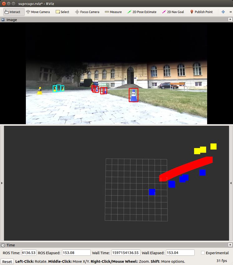
Example of the system can be found in Figures 8.2 and 8.3. The first one
captures the simulator itself. The second one captures visualization using
Rviz tool of what car sees and plans.
All days were live-streamed on the official FSO YouTube channel and can
be still accessed [16].
358. Formula Student Driverless Simulator ..........................
Figure 8.3: Rviz visualization
36Chapter 9
Radio-controlled Car
As a final platform used to validate the presented system and mainly control
algorithms, RC car was used. The ROS framework had to be adapted to this
platform again. The goal was to prove current system architecture working
with a focus on motion planning and trajectory tracking algorithm, so only
minor changes to the architecture were done.
9.1 System adaptation
The system in this application lacks an autonomous state machine because
it is redundant. CAN bus interface is replaced by interface for the RC car
which does not use CAN bus. For motion planning and trajectory tracking,
physical constants and tunable coefficients had to be changed. These were
done with respect to [2] where these were identified and tuned in simulation.
In the base architecture, cone detection is done using cameras and LIDAR.
The RC car is equipped only with one of the three cameras and has no LIDAR.
ZED camera, which is installed on both vehicles, is not at the same spot;
thus, the base system could not be used. Two significant changes had to be
made. The first was to gather images from the track from the new position of
the camera, label them, and train Neural Network (NN) using these pictures.
9.1.1 Cone detection
Cone detection is done with the YOLOv3 [17]. YOLOv3 offers a large number
of objects it detects. These are redundant in this specific use case, and desired
categories (blue, yellow, orange, and big orange cones) that are desired are
not part of the YOLOv3 output. As a standard procedure, the YOLOv3 was
changed, so it outputs only desired categories and then trained using a shared
database of labeled cones [18]. The approximate size of the training set is
8000 pictures. This NN is trained again using pictures obtained with RC car
to adapt to a new position, which is not represented in FSOCO database [18].
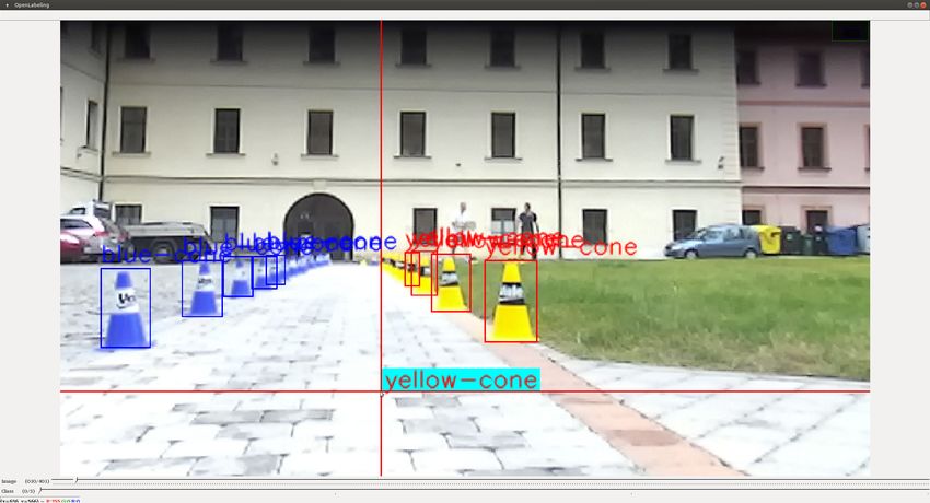
Over 350 images were captured and then manually labeled using OpenLa-
beling open-source labeler as labeling environment [19]. An example of the
environment is in Fig. 9.1.
37You can also read