Flow Simulation in a combined Region
←
→
Page content transcription
If your browser does not render page correctly, please read the page content below
E3S Web of Conferences 264, 01016 (2021)                                 https://doi.org/10.1051/e3sconf/202126401016
CONMECHYDRO - 2021

      Flow Simulation in a combined Region
      Umurdin Dalabaev*

      University of World Economy and Diplomacy, Tashkent, Uzbekistan

                    Abstract. The article deals with the flow in a complex area. The
                    composition of this region consists of a porous medium through the pores
                    of which the liquid moves and a zone without a porous framework (free
                    zone). The flow is modeled using an interpenetrating heterogeneous model.
                    In the one-dimensional case, an analytical solution is obtained. This
                    solution is compared with the solution learned by the move node method.
                    An analysis is made with experimental data with a Brinkman layer. A
                    numerical solution of a two-dimensional problem is also obtained.

      1 Introduction
      The flow of a liquid or gas in various media (porous and non-porous) occurs in a variety of
      applications. Such flows include, for example, the flow of gas and oil in and over a porous medium,
      underground hydrology, blood flow with stenosis, processes associated with movement through a
      rough surface, etc. e. Modeling the flow of such problems can be divided into two directions.
          The first direction is associated with Darcy's law for a porous layer and the Navier-Stokes
      equation in the pure region. In [1-6], the flow in the combined region was investigated using the
      Darcy and Stokes/Navier-Stokes model. In the Darcy model, it is believed that the flow inertia is
      small, and in the case of highly porous media and in large Reynolds numbers, the results of this model
      give large errors. At the interface between the porous medium and the isotropic region, the boundary
      conditions are set [7-10]. In the second approach, which is called one regional, the flow is described
      by a single equation (equations of the Darcy-Brinkman type) [11-16].
          In [17], the flow in the combined region is investigated by a numerical method and with the help
      of Darcy Brinkman, and a voluminous review of this topic is given.
          An experimental study is devoted to [18-19], in which the thickness of the interboundary layer is
      analyzed.
          Here it is proposed to describe the flow inside and outside the porous medium with a single
      equation using the model of two-phase media

      2 Methods
      Let us consider an interpenetrating model describing the flows of two-phase media [18-19], where the
      velocity of the discrete phase is neglected. Then the flow of the liquid phase is described by a system
      of equations (two-dimensional case):

      *Corresponding author: udalabaev@mail.ru

© The Authors, published by EDP Sciences. This is an open access article distributed under the terms of the Creative Commons
Attribution License 4.0 (http://creativecommons.org/licenses/by/4.0/).
E3S Web of Conferences 264, 01016 (2021) https://doi.org/10.1051/e3sconf/202126401016
CONMECHYDRO - 2021
u j 2 u j p 2 1
u j
u k f kj 1 f
t k 1 xk x j k 1 3 xk x k
(1)
5 u3 j
2
1 kj f Ku j g j ,
k 1 3 xk x3k
2 fuk
0. (2)
k 1 xk
Here, u j is the j-th component of the flow velocity, p is fluid pressure, f is volume
concentration, kj is the Kronecker symbol, is fluid viscosity, K is interaction
coefficient, is fluid density, g j is force terms accounting for gravity.
Suppose the equations are transformed into the integral form of representation, then on their basis. In
that case, it is possible to study flows both inside and outside porous media, since when f 1 we
obtain the Navier - Stokes equations for an incompressible fluid. Moreover, these equations
are suitable for the entire area under consideration.
3 Results and Discussion
Let us consider some one-dimensional problems of applying the model (1), (2).
3.1. Exact solution
Let a liquid flow in a flat pipe partially filled with a porous medium. The lower part of the horizontal
pipe is filled with a porous medium with height h (pipe height H). Assuming the flow to be one-
dimensional and stationary, we obtain from (1), (2)
du du dp
f Ku
f (3)
dy dy dx
In (3), for the parameter K, we use the Carman- Kozeny relation as adopted in porous media:
2
f
K (4)
k
2 3
d f
Where k 2
, permeability, d is the characteristic size of the porous
180(1 f )
medium.
2
rU
Let us pass to dimensionless variables by setting
u uU
, y yH , x xH , p p.
Re
Then equation (3) in dimensionless form at f const , has the form:
2E3S Web of Conferences 264, 01016 (2021) https://doi.org/10.1051/e3sconf/202126401016
CONMECHYDRO - 2021
2
d u dp
Au 2 (5)
dy dx
2 2 2
Here, A 180 H / d
(1 f ) / f .
In the free zone, the one-dimensional flow satisfies the equation
2
d u dp
(6)
2
dy dx
Further, in equations (5-6), drop the dash above the variables.
Equation (5) is considered when 0 y h0 , and equation (6) in h0 y 1 . Equations
are solved under the following boundary conditions. The no-slip conditions for equation (5)
in the lower wall and for equation (6) in the upper wall:
u (0) 0,
u(1) 0. (7)
In the interfacial condition, we set the conditions for flow continuity and equality of the
shear stress:
du ( h0 0) du ( h0 0)
u ( h0 0) u ( h0 0), (8)
dy dy
It is easy to obtain an analytical solution to (5) and (6) with the above boundary
conditions. Figure 1 shows the analytical solution. The dimensionless pressure drop is taken
so that it corresponds to a flow without a porous layer, a unit flow rate. The dotted line
corresponds to the solution obtained with a porosity of 0.3; the dotted line is 0.5.
Fig.1. Exact solution: velocity distributions Fig.2. Comparison of the results of accurate and
at different porosity values numerical results at different values of porosity
3.2 Numerical solution
Consider Eq. (5) for the entire region, and put
f
at 0 y h0
1 at h0 y 1
(9)
3E3S Web of Conferences 264, 01016 (2021) https://doi.org/10.1051/e3sconf/202126401016
CONMECHYDRO - 2021
In this case, equation (5) in the pure region takes the form (6). Thus, equation (5) can be
used in the entire region, with porosity (9), while the boundary conditions are fulfilled
automatically (in the porous layer, the porosity is taken equal to ). For this purpose, a
finite-difference approximation of equation (5) was made, and the calculation was
performed using the sweep method (using a special linear system solver designed to take
advantage of the tridiagonal structure of the coefficient matrix) in the combined domain.
Figure 2 shows the results of numerical calculations (solid curves, analytical solution,
point data, numerical results). This shows that it is possible to make an end-to-end
calculation without highlighting the borderline condition.
3.3 Influence of the pipe roughness thickness on the pressure drop
To influence the pipe roughness thickness on the pressure drop, we use a solution using an
analytical solution. To ensure a unit flow rate of liquid with a unit height of the flow based
on Poiselle's law for smooth pipes, it turns out that. Figure 3 shows graphs of the pressure
drop depending on the thickness of the porous layer.
Based on figure 3, it can be concluded that the nature of the change in the pressure drop
relative to the layer thickness does not depend on the porosity of the layer: it behaves like
an "S" shaped function. However, the range of variation strongly depends on the porosity.
3.4 An approximate analytical solution using a movable node.
Using the method of movable node [21], one can find an approximate analytical solution to
the problem.
a) f 0.8 b) f 0.5 v) f 0.3
Fig.3. Pressure drop versus layer thickness
Equation (5.6) is approximated by difference relations:
uG u u
2 dp
Au (9)
h h0 y y dx
0
2 u u uG dp
(10)
1 h0 1 y y h0 dx
4E3S Web of Conferences 264, 01016 (2021) https://doi.org/10.1051/e3sconf/202126401016
CONMECHYDRO - 2021
In the difference equations (9, 10), the no-slip boundary conditions are used. In
equations (9, 10) uG is the value of the unknown function on the interfacial boundary. To
find uG we use the second interfacial condition (8). Put in (9) y h0 0 , then we have
2
du u
dp
AuG (11)
h0 dy h 0 h0 dx
0
If in (10) y h0 0 then we have:
2 uG du dp
(12)
1 h0 1 h0 dy h0 0 dx
Using (8), we obtain
h0 (1 h0 ) dp
uG (13)
2
2 h0 (1 h0 ) dx
Using (13) from (9) and (10), we determine the distribution of velocities in the porous
y 2(1 h0 ) dp
u h0 y . (14)
2 h0 (1 h0 )
2
2 Ay ( h0 y )
dx
and free zones
1 y (1 h0 )( y h0 ) h0 (1 h0 ) dp
u
(15)
2
1 h0 2 2 Ah0 (1 h0 ) dx
In fig. 4, the exact and approximate solutions are compared (the solid line is the exact solution,
and the dotted line is approximate, obtained using (14) and (15)
at A 40000,
h0 0.2 ).
Fig.4. Comparison of solutions Fig.5. Comparison with experimen
5E3S Web of Conferences 264, 01016 (2021) https://doi.org/10.1051/e3sconf/202126401016
CONMECHYDRO - 2021
3.5 Comparison with experiment
In [22], the thickness of the Brinkman boundary layer was experimentally investigated. In
this layer, which is located between the Darcy layer and the layer with a pure region, based
on experimental data, an empirical formula is obtained
u uD
u exp( ( y 1)) (16)
uint u D
Here is u D the Darcy velocity, uint is the interfacial velocity,
3 4( y 1) ,
Figure 5 shows a comparison of the results obtained based on (5) and (6) (solid
line) and (16) for the transition layer.
To obtain a visual representation of the solution to the problem in the combined domain,
a numerical calculation was performed using equations (1-2) based on a similar SIMPLE
algorithm [19].
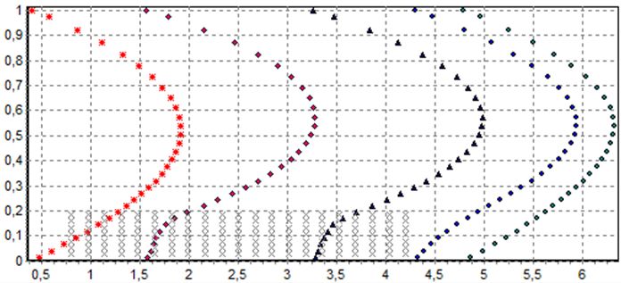
Fig.6. Longitudinal velocity profiles at different sections ( f 0.4).
In figure 6, the porous layer is located in the region 0.8 x 4.2; 0 y 0.1
porosity f 0.4. At the entrance, a parabolic law is given; in the sections inside
the porous layer, the profile is flattened, and a rapid increase in velocity begins to
occur (Re 21).
6E3S Web of Conferences 264, 01016 (2021) https://doi.org/10.1051/e3sconf/202126401016
CONMECHYDRO - 2021
Fig.7. Longitudinal velocity profiles at different sections ( f 0.8).
In figure 7 numerical results, the porosity of the layer is 0.8. In this case, Darcy's law does
not hold inside the layer. The irregularity of the velocity profile covers the entire porous
region. Visual comparison with experiment [23] gives good results concerning the
interfacial layer.
4 Conclusions
Rakhmatulin's model can be successfully applied to describe the flow in the combined
region. An approximate analytical solution obtained on the basis of the method of movable
nodes can be used to describe the flow for one-dimensional problems; to obtain more
accurate approximate solutions, it is possible to achieve multipoint movable nodes. The
results of the study are in good agreement with the experimental results. The results of test
calculations and the influence of grid parameters, reflecting the validity of the application
of the model and the proposed numerical approach, are presented.
References
1. William Jj. Llayton,, Friedhelm Schieweck,, and Ivan Yotov, Coupling fluid flow with
porous media flow, SIAM J. NUMER. ANAL., 40(6), pp. 2195–2218
2. Dayle Jogie1, Balswaroop Bhatt, Flow of immiscible fluids in a naturally permeable
channel, International Journal of Pure and Applied Mathematics, 78(3),pp 435-449
(2012)
3. Kirill Tsiberkin, Ekaterina Kolchanov, and Tatyana Lyubimov, Verification of the
boundary condition at the porous medium–fluid interface, EPI Web Conferences 114,
02125 (2016) DOI: 10.105/epjconf/ 201611402125. (2016).
4. Philippe Angot, Well-posed stokes, brinkman and stokes/darcy coupling revisited with
new jump interface conditions, Mathematical Modelling and Numerical Analysis,
ESAIM: M2AN 52 pp 1875-1911, https://doi.org/10.1051/m2an/2017060. (2018)
5. Matthias Ehrhardt, An Introduction to Fluid-Porous Interface Coupling, Progress in
computational physics, 2:3–12, 2000..
6. Fernando A. Moralesa,, Ralph E.Showalterb, A Darcy–Brinkman model of fractures
in porous media, Journal of Mathematical Analysis and Applications, J. Math. Anal.
Appl. 452 pp 1332–1358. (2017).
7. Beavers G. S., Joseph D. D., Boundary conditions at a naturally permeable wall, J.
Fluid Mech., 30 pp. 197-207. (1967),
7E3S Web of Conferences 264, 01016 (2021) https://doi.org/10.1051/e3sconf/202126401016
CONMECHYDRO - 2021
8. Saffman P. G. On the Boundary Condition at the Surface of a Porous Medium. Stadies
in Applied Mathematics, pp.93-101, https://doi.org/10.1002/sapm197150293. (1971)
9. J. Alberto Ochoa-Tapia, J. Whitaker.S. Momentum transfer at the boundary between
a porous medium and a homogeneous fluid-I. Theoretical development, International
Journal of Heat and Mass Transfer, 38(14), September 1995, pp 2635-2646,
https://doi.org/10.1016/0017-9310(94)00346-W. (1995)
10. J. Ochoa-Tapia, J.A., Whitaker, S., Momentum jump condition at the boundary
between a porous medium and a homogeneous fluid: inertial effect. J. Porous Media 1,
pp 201–217. (1998).
11. Yu, P., T.S., Zeng, Y. Low, Y. T. , A Numerical for flows in porous and homogenous
fluid domains coupled at the interface by stresss jump. Int. J. Numer. Meth. Fluids 53,
pp 1755-1775, https://doi.org/10.1002/fld.1383
12. Oleg Iliev and Vsevolod Laptev. On numerical simulation of flow through oil filters.
Computing and Visualization in Science, 6(2) pp 139–146, Mar 2004. ISSN 1433-
0369. doi: 10.1007/s00791-003-0118-8. URL https://doi.org/10.1007/s00791-003-
0118-8. (2004).
13. Ershin Sh. A, Zhapbasbayev U. K., Model of Turbulent Motion of Incompressible
Liquid in Apparatus with a Permeable Partition, Publishing House of the SB RAN:
Applied Mechanics and Technical Physics
14. Gaev E. A. Shikhaliev S. Z, Numerical study of fluid inlet into a channel with a linear
easily permeable roughness, Applied hydrodynamics, 4, (76), pp. 32-39.( 2002).
15. Dalabaev, U, Numerical investigation of the character of the lift on a cylindrical
particle in Poiseuille flow of a plane channel, 6 November 2011,
https://doi.org/10.1007/s10891-011-0609-2. (2011).
16. Dalabaev, U. Structure of flow through an immovable granular layer. J Eng Phys
Thermophys 70, pp 379–382 https://doi.org/10.1007/BF02662134. (1997).
17. Kazunori Fujisawa, Akira Murakami, Numerical analysis of coupled flows in porous
and fluid domains by the Darcy-Brinkman equations, Soils and Foundations, 58, (5),
October 2018, pp 1240-1259 https://doi.org/10.1016/j.sandf.2018.07.003. (2018).
18. Faizullaev, D. F, Laminar Motion of Multiphase Media in Conduits, Springer
US, ISBN 978-1-4899-4832-8 (1969).
19. Nigmatulin, R. I., Fundamentals of the mechanics of heterogeneous media, Moscow,
Izdatel'stvo Nauka, p 336. In Russian. (1978).
20. Patankar S. Numerical Heat Transfer and fluid Flow, ISBN 9780891165224 Published
January 1, by CRC Press.( 1980).
21. Dalabaev U. Computing Technology of a Method of Control Volume for obtaining of
the Approximate Analytical Solution one-dimensional Convection-diffusion
Problems. Open Access Library Journal, 5: 1104962..
https://doi.org/10.4236/oalib.1104962 (2018).
22. Mohammad Reza Murad, Arzhang Khalili, Transition layer thickness in a fluid-porous
medium of multi-sized spherical beds, Exp. Fluids 46:323-330, DOI 10/1007/s00348-
008-0562-9. (2009)
23. Afshin Goharzadeh, Arzhang Khalili, and Bo Barker Jorgensen, Transition layer
thickness at a fluid-porous interface, Physics of fluids 17: 057102, DOI
10.1063/1.1894756. (2005)
8You can also read