Growing synthetic data through differentially-private vine copulas
←
→
Page content transcription
If your browser does not render page correctly, please read the page content below
Proceedings on Privacy Enhancing Technologies ; 2021 (3):122–141

Sébastien Gambs, Frédéric Ladouceur, Antoine Laurent, and Alexandre Roy-Gaumond*

Growing synthetic data through
differentially-private vine copulas
Abstract: In this work, we propose a novel approach for           data portal3 and the American data portal4 , respec-
the synthetization of data based on copulas, which are            tively each with 83 460 and 209 765 datasets. The open
interpretable and robust models, extensively used in the          data movement has also led cities to open more and
actuarial domain. More precisely, our method COPULA-              more data. Concrete examples are the cities of Mon-
SHIRLEY is based on the differentially-private training           tréal5 and Toronto6 , with around 350 datasets each.
of vine copulas, which are a family of copulas allow-                  The major drawback of this augmentation in the
ing to model and generate data of arbitrary dimensions.           availability of data is that it is accompanied by the in-
The framework of COPULA-SHIRLEY is simple yet flex-               crease in privacy risks for the individuals whose records
ible, as it can be applied to many types of data while            are contained in the shared data. Such privacy risks
preserving the utility as demonstrated by experiments             have been demonstrated many times in the literature,
conducted on real datasets. We also evaluate the pro-             even in the situation in which the data was supposed
tection level of our data synthesis method through a              to be anonymized. For instance, in the context of mo-
membership inference attack recently proposed in the              bility data, researchers have shown that any individual
literature.                                                       is unique in a population with respect to his mobil-
                                                                  ity behaviour simply given three to five points of in-
Keywords: Synthetic data, Copulas, Differential privacy,
                                                                  terests (i.e., frequently visited locations) [17]. Follow-
Privacy evaluation.
                                                                  ing the same approach but in the context of financial
DOI 10.2478/popets-2021-0040                                      data, another study has demonstrated that five credit
Received 2020-11-30; revised 2021-03-15; accepted 2021-03-16.     card transactions are sufficient to uniquely pinpoint an
                                                                  individual [18]. Finally, even data that appears to be
                                                                  “harmless” at first sight such as movie ratings could
1 Introduction                                                    lead to privacy risks as illustrated by Narayanan and
                                                                  Shmatikov [48, 59].
With the advent of Big Data and the widespread de-                     To address these issues, multiple anonymization
velopment of machine learning, the sharing of datasets            techniques have been developed in the last two decades.
has become a crucial part of the knowledge discovery              Among these, there has recently been a growing interest
process. For instance, Kaggle1 , a major actor in the             in generative models and synthetic data. A key prop-
data portal platforms, supports more than 19 000 pub-             erty of generative methods is their ability to mince even
lic datasets and the University of California at Irvine           more the link between identities and the data shared in
(UCI)2 repository is another important data portal with           comparison with other anonymization techniques. This
more 550 curated datasets that can be used for ma-                property is due to the summarization of the data to
chine learning purposes. Numerous public institutions             probabilistic representations that can be sampled to
also publicly share datasets such as the Canadian open            produce new profiles that are not associated with a par-
                                                                  ticular identity. Nonetheless, generative models as well
                                                                  as the synthetic data they produce, can still leak infor-
                                                                  mation about the dataset used to train the generative
Sébastien Gambs: UQAM, E-mail:
gambs.sebastien@uqam.ca
                                                                  model and thus lead to privacy breaches. In particular,
Frédéric Ladouceur: Ericsson Montréal, E-mail:                    a recent study by Stadler, Oprisanu and Troncoso [62]
ladouceu@stanford.edu                                             have demonstrated that generative models trained in
Antoine Laurent: UQAM, E-mail: lau-
rent.antoine@courrier.uqam.ca
*Corresponding Author: Alexandre Roy-Gaumond:
UQAM, E-mail: roy-gaumond.alexandre@courrier.uqam.ca              3   https://open.canada.ca/en/open-data
                                                                  4   https://www.data.gov/
1 https://www.kaggle.com/datasets                                 5   https://donnees.ville.montreal.qc.ca/
2 https://archive.ics.uci.edu/ml/datasets.php                     6   https://open.toronto.ca/
Growing synthetic data through differentially-private vine copulas 123
a non-private manner provide little protection against ing data in a private manner. Most of these methods
inference attacks compared to simply publishing the rely on generative models that condense the information
original data. They also showed that generative models in probabilistic models, thus severing the link between
trained in a differentially-private manner did not im- identity and data through randomness and abstrac-
prove the protection. tion. Common generative models include Bayesian net-
Thus, in addition to being based on a formal model works [32], Markov models [63] and neural networks [4].
such as differential privacy, we believe that data synthe- It is possible to roughly distinguish between two types
sis methods should be assessed with a privacy evalua- of synthesis methods: partial and complete.
tion based on inference attacks to further quantify the Partial data synthesis. Partial synthesis implies
privacy protection provided by the synthesis method. that for a given profile, some attributes are fixed while
In this paper, we propose a copula-based approach to the rest is sampled by using the generative model. As
differentially-private data synthesis. Our approach aims a consequence partial synthesis requires both the access
at providing an answer to the following conundrum:How to part of the original profiles and the trained generative
to generate synthetic data that is private yet realistic model.
with respect to the original data? A seminal work on partial data synthesis is done by
The proposed generative model is called COPULA- Bindschadler, Shokri and Gunter in [11], in which they
SHIRLEY, which stands for COPULA-based genera- develop a framework based on plausible deniability and
tion of SyntHetIc diffeRentialL(E)Y-private data. In a differential privacy. The generative model used is based
nutshell, COPULA-SHIRLEY constructs a differentially- on differentially private Bayesian networks capturing
private vine copulas model that privately summarizes the joint probability distribution of the attributes. In a
the training data and can later be used to generate syn- nutshell, the “seed-based” synthesis of new records takes
thetic data. We believe that our method has the follow- a record from the original dataset and “updates” a ran-
ing strengths: dom subset of its attributes through the model. Their
– Simple to use and deploy - due to the nature of the approach releases a record only if it passes the privacy
mathematical objects upon which it is based, which test of being similar to at least k records from the orig-
are mainly density functions. inal dataset, hence the plausible deniability. A notable
– Flexible - due to the highly customizable framework drawback of this approach is the high computational
of copulas and their inherent ability to model even time and the large addition of noise, which makes it dif-
complex distributions by decomposing them into a ficult to scale to high-dimensional datasets as pointed
combination of bivariate copulas. out in [15].
– Private - due to the use of differential privacy to In contrast, complete synthesis methods output new
train the generative model as well as the privacy profiles directly from the generative model. Hereafter,
test for membership inference. we focus on complete data synthesis methods.
Statistical-based generation. The PrivBayes ap-
The outline of the paper is as follows. First, we re- proach [77] has become one of the standards in the lit-
view the literature on differentially-private data syn- erature for complete data synthesis through Bayesian
thesis methods in Section 2 before presenting the back- networks. PrivBayes integrates differential privacy in
ground notions of differential privacy and copulas theory each step of the construction of the Bayesian network
in Section 3. Afterwards, we describe in detail in Sec- while optimizing the privacy budget. More precisely, the
tion 4 the synthesis based vine copulas that we propose construction applies the Exponential mechanism on the
COPULA-SHIRLEY, followed by an experimental evalu- mutual information between pairs of attributes and the
ation of the utility-privacy trade-off that it can achieve Laplace mechanism to protect the conditional distribu-
on three real datasets in Section 5 before concluding. tions [22]. Moreover, the privacy of the method relies
solely on the use of differential privacy and no inference
attacks are provided. In addition, the greedy construc-
tion of the Bayesian network is time consuming, which
2 Related work on private data makes it impractical for high-dimensional data.
synthesis Gaussian models are widely used for data mod-
elling, independently of the properties of the data it-
Although the literature on anonymization methods is self, as the structure of the data can be accurately
huge, hereafter we focus on the methods for synthesiz- estimated with only the mean and covariance of theGrowing synthetic data through differentially-private vine copulas 124
data. Recently Chanyaswad, Liu and Mittal have pro- GAN-based generation. Since the influential
posed a differentially-private method to generate high- work of Goodfellow and collaborators [28] on Genera-
dimensional private data through the use of random tive Adversarial Networks (GANs), this approach has
orthonormal projection (RON) and Gaussian models been leveraged on for private data generation [24, 34,
named RON-Gauss [15]. RON is a dimensionality reduc- 67, 70, 75] to name a few. For instance, the work of Jor-
tion technique that lowers the amount of noise added to don, Yoon and van der Schaar has introduced PATE-
achieve differential privacy and achieves the Diaconis- GAN [34], which combines two previous differentially-
Freedman-Meckes (DFM) effect stating that “under private machine learning techniques of machine learn-
suitable conditions, most projections are approximately ing, namely Private Aggregation of Teacher Ensembles
Gaussian”. With the DFM effect, Gaussian generative (PATE) [50] and Differentially Private Generative Ad-
models are then well suited to model the projected data versarial Network (DPGAN) [74]. The combination of
and are easily made differentially private. The authors these two is done by using a “student” layer that learns
have implemented the membership inference attack de- from the differentially-private classifier PATE as the dis-
scribed in [58] as a privacy test and shown that with a criminator in the DPGAN framework, thus enabling the
privacy budget < 1.5 the success of the attack is no training of both a differentially-private generator and
better than a random guess. discriminator. The work of [34] advocates the privacy
Copula-based generation. Comparable works to of their synthetic records because of the use of differen-
our use copula functions as generative models [6, 36]. To tial privacy but do not use any privacy tests to validate
the best of our knowledge, the first differentially-private it. The main disadvantages of using techniques such as
synthesis method based on copulas is by Li, Xiong and GANs are that they need a large quantity of data, a fine-
Jiang and is called DP-COPULA [36]. The authors have grained tuning of their hyper parameters and they have
used copulas to model the joint distributions based on a high complexity, which makes them inappropriate for
marginal distributions. They use differentially-private a number of real-life applications.
histograms as marginal distributions and the Gaussian Privacy evaluation. The amount of data synthe-
copula to estimate the joint distribution. No privacy sis methods based on generative models trained in a
tests on their differentially-private synthetic data was differentially private manner as grown significantly in
considered by the authors and much like RON-Gauss recent years. However, a fundamental question to solve
[15], they simplify the structure to a Gaussian model. when deploying these models in practice is what value
However, some authors have shown that some tail de- of to choose to provide an efficient protection. While
pendencies are not fully capture by Gaussian models, there is currently no consensus on the “right value” of
which can lead to an important loss of information [38]. , often researchers set ∈ (0, 2] but it can sometimes
In contrast, as described in Section 3.2, vine copulas, be greater than > 105 [37, 46, 50]. Moreover, a recent
which are the basis of COPULA-SHIRLEY, split the mul- study has shown the importance of providing a privacy
tivariate function into multiple bivariate functions en- assessment even when the model is trained in a differen-
abling the bivariate families of copulas to successfully tial privacy manner [62]. In particular, the authors have
capture the dependence structure. demonstrated that differential privacy in model train-
Tree-based generation. A vine copula is a struc- ing does not provide uniform privacy protection and
ture with nested trees, which can thus be viewed as that some models fail to provide any protection at all.
a tree-based generation model (TGM). Other PGMs Thus, while achieving differential privacy is a first step
for synthetic data generation such as Reiter’s work [55] for data synthesis, we believe that it is also important
and [14] rely on trees to model the conditional proba- to complement them with methods that can be used
bilities between a variable Y and some other predictor to evaluate the remaining privacy risks of sharing the
variables Xi , in which i varies from 1 to n, the number synthetic data.
of attributes. More precisely, each leaf corresponds to a To the best of our knowledge, very few works on
conditional distribution of Y given ai ≤ Xi ≤ bi . Such data synthesis achieving differential privacy have also
an approach can be classified as partial data synthesis proposed methods to assess the remaining privacy risks
due to the use of the predictor variables to form the related to synthetic data with the exception of [11],
imputed synthetic Y . In comparison, the nested trees of which assesses the plausible deniability level of the gen-
vine copulas have the advantages to provide fully syn- erated data. Privacy can be assessed in multiple ways.
thetic data as well as deeper modelling of conditional A common approach when using differential privacy,
distributions due to a more flexible representation. which mitigates the risk of membership disclosure riskGrowing synthetic data through differentially-private vine copulas 125
by diminishing the contribution of any individual in the based on the notation used in the book of Dwork and
model learned, is testing via membership inference at- Roth [22].
tacks. A recent paper [30] proposed a model-agnostic
method to assess the membership disclosure risk by Definition 3.1 (Differential privacy (bounded)). Let
quantifying the ease of distinguishing training records x and y two databases of equal size such that they differ
from other records drawn from a disjoint set with the at most by one record. A randomized mechanism M is
same distribution. -differentially private such that for the space of possible
In the machine learning context, the approach outputs S ⊆ =(M) we have:
recently developed by Meehan, Chaudhuri and Das-
Pr[M(x) ∈ S] ≤ exp() · Pr[M(y) ∈ S].
gupta [43] tackled the data-copying issue that can arise
from generative models. Data-copying is defined as a
This property ensures that the difference in the outputs
form of overfitting in which trained models output iden-
of the randomized mechanism is indistinguishable up
tical or very similar profiles to the training samples. The
to exp() for two databases that differ in at most one
proposed framework focuses on global and local detec-
profile. Here, is the parameter defining the level of
tion of data-copying by measuring the distribution of
privacy. In particular, the smaller is the value of , the
distances between the synthetic profiles and their near-
higher is the protection offered due to the increase in
est neighbours in the training set as well as in a test set.
indistinguishability.
The main idea here is that a smaller distance between
The (global) sensitivity ∆ of a function f is an im-
the synthetic profiles and the training ones compared
portant notion in differential privacy formalizing the
to the synthetic to test ones is an indication that the
contribution of a particular individual on the output
data generation process has a tendency to exhibit data-
of this function. More precisely, the sensibility charac-
copying.
terizes the answer to the following question: “What is
the maximal contribution that an individual can have
on the outcome of a particular function f ?”.
3 Preliminaries For an arbitrary function f , there exists many ways
to make it -differentially private. For instance, the
In this section, we review the background notions nec- Laplacian mechanism [22] can be used to make a numer-
essary to the understanding of our work, namely dif- ical function returning a real or a set of reals f : D → Rk
ferential privacy as the privacy model upon which our -differentially private by drawing randomly from the
method is built as well as copulas and vine copulas as Laplacian distribution Lap( ∆f ).
the underlying generative model. Another important concept in differential privacy is
the notion of the privacy budget, which bounds the total
amount of information leaked about the input database
3.1 Differential privacy when applying several mechanisms on this database.
The application of several mechanisms do not always
Differential Privacy (DP) is a privacy model that aims have the same impact on the privacy budget depending
at providing strong privacy guarantees with respect to on whether these mechanisms are applied in a sequential
the amount of information that can leak about individ- or parallel manner. The following theorems are inherent
uals that are part of a database [22]. In a nutshell, DP properties of differential privacy and help to adequately
ensures that the contribution of a particular profile will manage the privacy budget.
have a limited impact on the outcome of a computation In the following, R and R0 are arbitrary sets, which
run on the input database. This property is achieved refer to the image of the functions defined in the theo-
by ensuring (e.g., through the addition of noise to the rems.
output or by randomizing the computation) that the
distribution of outputs of the computation or the query Theorem 3.1 (Closure under post-processing [22]).
is “almost the same” whether or not the profile of an Let M : D → R be a -differentially private randomized
individual was in the input database. mechanism and f : R → R0 be an arbitrary function,
For our framework, we use the bounded defini- independent of D, then the composition f ◦ M : D → R0
tion of differential privacy. The following definitions are is also -differentially private.Growing synthetic data through differentially-private vine copulas 126
A subtle but important point of Theorem 3.1 of the Estimating the copula function with a known distribu-
closure under post-processing is that the function f has tion family results in modelling the dependence struc-
to independent of D, which means that it should not ture of the data. Assuming a variable of interest of di-
have access to or use any information about D. If this mension n, the modelling by copula is generally done by
is not the case, the theorem does not apply anymore. first choosing a family of copulas and then verifying the
“goodness-of-fit” of this modelling, in the same manner
Theorem 3.2 (Sequential composition [22]). Let M1 : that a known distribution can be used to estimate an
D → R and M2 : D → R0 be two randomized mecha- arbitrary distribution.
nisms that are respectively 1 and 2 -differentially pri- Figure 1 [27] illustrates simulations from five com-
vate, then the composition (M1 , M2 )(x) : D → R × R0 mon bivariate copulas and the tail dependence they help
is (1 + 2 )-differentially private. to model. We refer the interested reader to [33, 49] for
further reading about the many existing families of cop-
Theorem 3.3 (Parallel composition [22]). Let M1 : ulas and their tail dependence modelling (each of these
D1 → R and M2 : D2 → R0 be two randomized mech- books defines and discusses more than 20 families of
anisms that are respectively 1 and 2 -differentially pri- copulas).
vate, such that D1 , D2 ⊂ D and D1 ∩ D2 = ∅, then the
composition (M1 , M2 )(x) : D → R × R0 is max(1 , 2 )-
differentially private.
Theorems 3.2 and 3.3 can easily generalized to k sequen-
tial mechanisms or disjoint subsets.
3.2 Copulas and vine copulas
Copulas. Historically, copulas date back from 1959
with Abe Sklar that has introduced this notion in his
seminal paper [60] at which time they were mainly theo-
retical statistical tools. However, in the last decade they
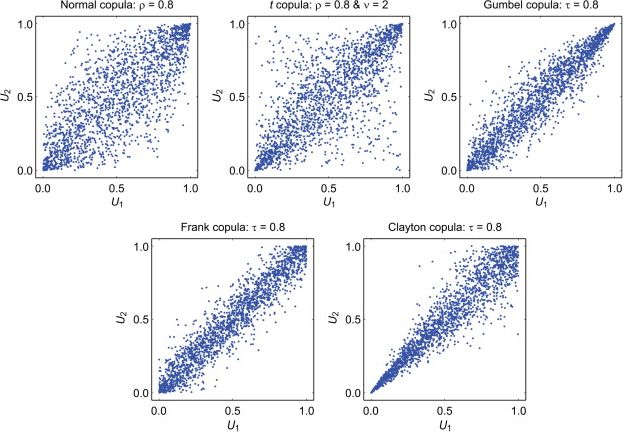
have experienced a significant growth in many domains Fig. 1. Simulations from common copulas family.
including earth science for modelling atmospheric pre-
cipitation [8], in health for diagnostic tests [31], in fi-
nances for the study of financial time series [51], in social Sklar’s theorem is a fundamental tool in copula the-
sciences for modelling the different usages of a technol- ory that binds together the marginals and the copula,
ogy [35], in genetics for the study of phenotypes [29] and which means that we only need the marginals of the
even more recently in privacy for estimating the risk of data to model the dependence structure.
re-identification [56].
Theorem 3.4 (Sklar’s Theorem [60]). Let F be
In a nutshell, a copula is a multivariate Cumula-
a multivariate cumulative distribution function
tive Density Function (CDF) on the unit cube with the
with marginals FXi with i ∈ {1, 2, . . . , n}.
marginal distributions (or simply marginals) on its axes
Then, there exists a copula C such that
modelling the dependence between the said marginals.
F (X1 , X2 , . . . , Xn ) = C(FX1 , FX2 , . . . , FXn ). If all
The formal definition of a copula is as follows:
the marginals are continuous, then C is unique.
Definition 3.2 (Copula [49]). Let (X1 , X2 , . . . , Xn ) be Conversely, if FXi are univariate distribution func-
a random vector such as the associated cumulative tions and C is a copula, then C(u1 , u2 , . . . , un ) =
−1 −1 −1
density functions FXi are continuous. The copula of F (FX 1
(u1 ), FX 2
(u2 ), . . . , FXn )−1 (un )) with FX i
being
(X1 , X2 , . . . , Xn ), denoted by C(U1 , U2 , . . . , Un ), is de- the inverse CDF of FXi .
fined as the multivariate cumulative density function of
Finally, a last fundamental theorem of the domain of
(U1 , U2 , . . . , Un ) in which Ui = FXi (Xi ) are the standard
copulas is the Probability Integral Transform (PIT) as
uniform marginal distributions of (X1 , X2 , . . . , Xn ).
well as the Inverse PIT.Growing synthetic data through differentially-private vine copulas 127
Theorem 3.5 (PIT [19]). Let X be a random variable With this definition, each edge e ∈ Ei is associated
with FX as its cumulative density function (CDF). The to (the density of) a bivariate copula cje ,ke |De , in which
variable Y = FX (X) is uniform standard. je , ke are the conditioned variables over the condition-
ing variables set De . Thus, the conditioned variables
Theorem 3.6 (Inverse PIT [19]). Let U be a uniform and the conditioning set form the conditional variables
standard random variable and F an arbitrary CDF, then Uje |De and Uke |De . The existence of such conditional
Y = F −1 (U ) is a random variable with F as its CDF. variables is guaranteed by the conditions on the trees
Ti , i ∈ {1, 2, . . . , n − 1} [9, 20].
The PIT and its inverse are used to transform data into To help visualize what is a vine, Figure 2 [1] shows
uniform standard distribution for the copulas to model an example of a vine on 5 variables. In this example, on
and back into the original domain after the generation the tree T4 , the conditioned variables are 1 and 5 and the
of new observations. conditioning set is {2, 3, 4} forming the variables U1|2,3,4
When applied on experimental data, uniform stan- and U5|2,3,4 .
dard marginals take the form of pseudo-observations
(i.e., normalized ranked data) that are computed via
the PIT. The pseudo-observations are then used to find
the best fitted copula model. Figure 1 illustrates such an
example in which data points (i.e., pseudo-observations)
are shown to best fit various copula models. The vine
copulas described hereafter offer a more refined manner
to describe the dependency structure.
Vine copulas. Vine copulas were introduced by
Bedford and Cooke in the early 2000s to refine the mod-
elling capabilities of copulas [9, 10]. The principle be-
hind them is simple: they decompose the multivariate
functions of the copula into multiple “couples” of cop- Fig. 2. Example of a vine on 5 variables.
ulas. A vine on n variables is a set of nested connected
trees (T1 , T2 , . . . , Tn ) such that edges of a tree Ti corre-
From a vine V , it is possible to describe a multivari-
sponds to vertexes in the following tree Ti+1 . Regular
ate density function as the product of bivariate copulas.
vines refer to a subset of vines constructed in a more
The following theorem implies that the joint density of a
constrained way. As we only use regular vines in this
multivariate random variables can always be estimated
paper, the term “vines” will refer to regular vines here-
via vine copulas.
after.
Theorem 3.7 (Vine density decomposition [9]). Let
Definition 3.3 (Regular vine [9]). A regular vine on n
V be a vine on n variables, then there is a unique
variables contains n − 1 connected nested trees denoted
density function f such as
T1 , T2 , . . . , Tn−1 . Let Ni and Ei be the set of nodes and
n
edges of the tree Ti . These trees satisfy the following Y
f (X1 , X2 , . . . ,Xn ) = fi (Xi )
properties:
i=1
1. T1 is the tree that contains n nodes corresponding n−1
to the n variables.
Y Y
cje ,ke |De Uje |De , Uke |De
2. For i ∈ {2, 3, . . . , n − 1}, the nodes set of Ti is such m=1 e∈Em
as Ni = Ei−1 .
3. For i ∈ {2, 3, . . . , n−1}, {a, b} ∈ Ei with a = (a1 , a2 ) in which Uje |De = Fje |De (Xje |De ) and Uke |De =
and b = (b1 , b2 ), it must hold that |a ∩ b| = 1. Fke |De (Xke |De ).
Condition 3. is called the proximity condition and can Formal and thorough definitions of vine copulas are
be translated to two nodes in tree Ti are connected by available in [9, 10, 20].
an edge if and only if these nodes, as edges, share a The construction of a vine is non-trivial as there are
approximately n! (n−2
2 ) different vines on n variables.
common node in tree Ti−1 . 2 ·2
The current state-of-the-art technique of constructionGrowing synthetic data through differentially-private vine copulas 128
uses a top-down greedy heuristic known as the Diss- of the Lasso [69] method and the use of Reinforcement
mann’s algorithm [20]. Learning (RL) with Long Short Term Memory net-
Dissmann’s algorithm for vine copula selec- works (LSTM) for near-optimal vine selection. Another
tion. The technique known as the Dissmann’s algorithm approach found in the literature uses auto-encoders
[20] is based on the hypothesis that the top of the tree on the data (here it could be used on the private
is more important in modelling the data than the lower pseudo-observations) to mitigate the curse of dimension-
branches as they contain raw information about the cor- ality [66]. A recent paper proposed a differentially pri-
relation between attributes. Dissmann’s algorithm can vate graphical model for low-dimensional marginals [42]
be summarized as: that could also be beneficial to our work. This work
1. Choose the optimal tree that maximizes the sum of defines an ad hoc framework for accurately and pri-
correlation coefficients between variables. vately estimate marginals and improve existing genera-
2. Choose the optimal copula family for each pair of tive models such as PrivBayes. We leave the investiga-
attributes (imposed by the tree) that minimizes the tion of these approaches as future works.
information loss.
3. Construct all the following trees (from the previous
optimal tree) that respect the regular vine defini-
tion 3.3 and return to Step 1. or stop if no tree can
4 COPULA-SHIRLEY
be constructed.
COPULA-SHIRLEY is a simple and flexible framework
for private data synthesis through vine copulas. In this
Step 1 is done by computing all the possible linear trees
section, we will first provide an overview of the algo-
(i.e., paths) and assigning to each edge the correlation
rithm, before describing in detail each of its subcompo-
coefficients between the two variables represented by the
nents. Finally, we present our privacy analysis as well
vertices. The path with the maximal sum of the corre-
as the membership inference attack that we have used
lation coefficients is chosen. For Step 2, each pair of
to evaluate the privacy level provided by our method.
attributes linked in the path are fitted on bivariate cop-
ula functions and the best fitted one is chosen using a
model selection criterion (such as Akaike Information
4.1 Overview
Criterion [3] or Bayesian Information Criterion [57]).
Note that due to the sequential aspect of the algo- Algorithm 1 outlines the framework of our method. The
rithm, it can be stopped at any level [12]. A truncated COPULA-SHIRLEY algorithm takes as input a dataset
vine copula will have independent bivariate copulas to D as well as a parameter , representing the privacy
model the conditional variables for all the trees below budget. The last two input parameters of COPULA-
the threshold. We will refer to the truncation level as SHIRLEY, nGen and EncodingM ethod correspond re-
Ψ. spectively to the number of synthetic data points to
The complexity of this heuristic lies on the fitting generate and which method of encoding for the categor-
of n bivariate copulas on the first tree T1 , n − 1 copulas ical attributes to use.
on the second tree T2 and so on until the last bivariate Note that copulas are originally mathematical ob-
copula on the last tree Tn−1 , in which n is the number jects used for modelling continuous numerical variables.
of attributes. If e(m) is the complexity of estimating a This means that the application of copulas to categori-
bivariate copula given m records, then the complexity of cal attributes requires an adequate preprocessing of the
the Dissmann’s algorithm is given by O(e(m) × n × Ψ). data, which is done by the P reprocessing function. Us-
The critical drawback of a sequential heuristic such ing the preprocessed data, the algorithm can tackle the
as Dissmann’s algorithm is that reaching the optimal task of building a vine copula for modelling the data in a
solution is not guaranteed, in particular for high dimen- differentially-private manner. Afterwards, this vine cop-
sions. Moreover, the greedy algorithm needs to compute ula can be sampled for producing new synthetic data.
the spanning tree and to choose a copula family for ev-
ery pair of nodes at each level of the vine leading to
important computational time with the increase in di- 4.2 Preprocessing
mensionality.
Recent advances regarding vine copulas construc- As directly cited from [36]: “Although the data should
tion such as [45] and [65] propose respectively the use be continuous to guarantee the continuity of margins,Growing synthetic data through differentially-private vine copulas 129
Algorithm 1: COPULA-SHIRLEY erence attribute given the (encoded) attribute’s value.
Input: Dataset: D, global privacy budget: , The GLMM can be seen as an extension of logistic re-
number of records to generate: nGen, gression in which the encoding of an attribute is com-
encoding method : EncodingM ethod puted by the expected value of an event (i.e., encoded
Output: Differentially-private synthetic attribute) given the values of the predictor.
records: Dsyn The preprocessing method shown in Algorithm 2
1 (pseudoObs, dpCDF s) ←− converts categorical values into dummy variables (if nec-
Preprocess(D, , EncodingM ethod) essary), computes the differentially-private CDFs from
(Section 4.2) the noisy histograms and outputs the noisy pseudo-
2 vineM odel ←− SelectVineCopula(pseudoObs) observations needed for the vine copula model construc-
(Section 4.3) tion. In the following, we describe in more details these
3 Dsyn ←− different processes.
GenerateData(vineM odel, nGen, dpCDF s) Split training. Since our framework needs two
(Section 4.4) sequential training processes: learning differentially-
4 return Dsyn private cumulative functions and learning the vine-
copula model, we rely on the parallel composition (The-
orem 3.3) of differential privacy by splitting the dataset
discrete data in a large domain can still be considered D into two subsets instead of using the sequential com-
as approximately continuous as their cumulative density position (Theorem 3.2) and splitting the global bud-
functions do not have jumps, which ensures the conti- get . In this manner, we efficiently use the modelling
nuity of margins.” This implies that if treated as con- strengths of copulas functions by sacrificing data points
tinuous, discrete data can be modelled with copulas. to reduce the noise added via the differentially-private
Thus, copulas can be used to model a wide range of mechanism (such as the Laplacian mechanism) while
data without the need of much preprocessing. However, preserving much of the data’s utility. Algorithm 2, line 3
an important issue arises when copulas are applied on shows the process of splitting the dataset into two sub-
categorical data as such data do not have an ordinal sets.
scale and copulas mostly use rank correlation for mod-
elling. In this situation, one common trick is to view Algorithm 2: Preprocessing
categorical data simply as discrete data in which the Input: Dataset: D, global privacy budget: ,
order is chosen arbitrarily (e.g., by alphabetical order), encoding method : EncodingM ethod
which is known as ordinal encoding. This trick has been Output: Differentially-private
proven to be a downfall for vine copula modelling for pseudo-observations: pseudoObs,
some metrics, as it will be discussed in Section 5. differentially-private CDFs: dpCDF s
Another technique to deal with categorical at- 1 D ← EncodingMethod(D)
tributes is the use of dummy variables, in which cat- 2 (dpT rainSet, modelT rainSet) ←
egorical values are transformed into binary indicator SplitDataset(D)
variables [64] (this technique is also known as one-hot 3 dpHistograms ←
encoding). The use of dummy variables helps preserve ComputeDPHistograms(dpT rainSet, )
the rank correlation between the attributes used by the 4 foreach hist in dpHistograms do
copulas (pseudo-observations). 5 cdf ← CumulSum(hist[binCounts])
Sum(hist[binCounts])
Two other supervised encoding techniques known
6 dpCDF s[col] ← cdf
as the Weight of Evidence (WOE) encoding [72] and
the Generalized Linear Mixed Model (GLMM) encod- 7 foreach col in modelT rainSet do
ing [13, 71] have been evaluated. Both need a reference 8 cdf ← dpCDF s[col]
attribute (called a predictor) and encode the categori- 9 pseudoObs[col] ← cdf (modelT rainSet[col])
cal attributes in a way that maximizes the correlation 10 return (pseudoObs, dpCDF S)
between the pair of encoded and reference attributes.
The WOE encoder can only be used with a binary ref-
erence attribute and is computed using the natural log Computation of DP histograms. The estima-
of the number of 1’s over the number of 0’s of the ref- tion of differentially-private histograms is the key pro-Growing synthetic data through differentially-private vine copulas 130
cess of COPULA-SHIRLEY. The current implementation use of vine copulas in such context is more complex, as
computes naively a differentially-private histogram by for each pair of copulas, a noisy estimation of its pa-
adding Laplacian noise of mean 0 and scale ∆ with ∆ = rameters is required, which results in an overall huge
2 to each bin count of every histogram (in the bounded injection of noise. Such a framework would also need a
setting of DP, the global sensitivity ∆ of histogram com- differentially-private implementation of the Dissmann’s
putation is 2). A more sophisticated method, such as algorithm, which is a complex task.
the ones defined in [2, 73, 76], could possibly be used to In contrast, COPULA-SHIRLEY reduces consider-
improve on the utility of the synthetic data. ably the noise added and the complexity of the im-
Computations of CDFs. Cumulative and proba- plementation by computing the dependencies on the
bility density functions are intrinsically linked together noisy marginal densities rather than on the original
and it is almost trivial to go from one to another. With data, thus enabling the use of vine copulas in a pri-
continuous functions, CDFs are estimated via integra- vate manner. COPULA-SHIRLEY is generic in the sense
tion of the PDF curves. In a discrete environment like that it can be used with any tree or copula selection
ours, as we use histograms to estimate PDFs, a sim- criterion, any algorithm for vine construction and any
ple normalized cumulative sum over the bin counts pro- method for differentially-private histograms or PDFs.
vides a good enough estimation of the CDFs, which is The complexity of COPULA-SHIRLEY is mainly im-
shown on line 6 of Algorithm 2. This is similar to the pacted by the algorithm for selecting the vine copula as
approach proposed by the Harvard University Privacy the complexity of ComputeDPHistograms, ComputeCDFs
Tools Project in the lecture notes about DP-CDFs [44], and ComputePseudoObs is O(nd), in which n is the num-
in which they add noise to the cumulative sum counts ber of profiles and d is the number of attributes (i.e., di-
and then normalize. Our method always produces a mensions) describing each profile. This latest cost is neg-
strictly monotonically increasing function, whereas their ligible compared to the cost of Dissmann’s algorithm.
approach tends to produce non-monotonic jagged CDFs.
A strictly monotonic increasing function is desirable
Algorithm 3: SelectVineCopula
as it means that the theoretical CDF always has an
inverse. Non-monotonic jagged CDFs can produce er- Input: Pseudo-observations: pseudoObs
ratic behaviours when transforming data to pseudo- Output: Vine Copula Model: vineM odel
1 vineM odel ←
observations and especially when mapping back to the
natural scale with the inverse CDFs. DissmannVineSelection(pseudoObs)
Computation of pseudo-observations. As cop- (Section 3.2)
2 return (vineM odel)
ulas can only model uniform standard marginals (i.e.,
pseudo-observations, we need to transform our data.
Easily enough, the PIT states that for a random vari-
able X and its CDF FX , we have that FX (X) is uniform Algorithm 3 outlines the general process for the
standard. Algorithm 2 does this at lines 8-10 by first ex- vine selection. As stated earlier, our method only needs
tracting the corresponding CDF (line 9) before applying the differentially-private uniform standard pseudo-
the said CDF onto the data (disjoint from the set used observations in order to select a vine. Dissmann’s al-
for computing the CDFs) (line 10). gorithm is then used with the noisy observations, and
only these observations, to fit the best vine copula. The
current implementation of COPULA-SHIRLEY uses the
4.3 Construction of the vine copula implementation of Dissmann’s algorithm from the R li-
brary rvinecopulib [47]. It offers a complete and highly
The two existing previous works at the intersection of configurable method for vine selection as well as some
differential privacy and copulas are restricted to Gaus- optimization techniques for reducing the computational
sian copulas [6, 36] because it makes it easier to build time for building the vine.
them in a differentially private manner. Indeed, it is pos-
sible to represent a Gaussian copula by the combination
of a correlation matrix and the marginal densities. In 4.4 Generation of synthetic private data
such case, it is enough to introduce appropriate noise
in these two mathematical structures to obtain a cop- The last step of our framework is the generation
ula model that is differentially-private by design. The of synthetic data. To realize this, uniform standardGrowing synthetic data through differentially-private vine copulas 131
observations must be sampled from the vine copula pseudoObs, we simply apply the differentially-private
model selected via the previous method. As we use the CDFs to the held-to model training set. The resulting
rvinecopulib implementation of the vine selection al- pseudoObs data is -differentially-private due to the ap-
gorithm, we naturally use their implementation of the plication of a -differentially-private mechanism and by
observation sampling from vines. Line 1 of Algorithm 4 the Parallel Composition theorem.
refers to the implementation of this sampling. We re- DissmannVineSelection only uses the -differentially-
fer the interested reader to [20] for more details about private set of data pseudoObs for its selection, resulting
how to sample from nested conditional probabilities as in a -differentially-private vine structure by the Closure
defined by the vine copula structure. Under Post-Processing property. Both, SampleFromVine
To map the sampled observations back to their and InverseFunction only use private data and therefore
original values, we use the Inverse Probability Integral do not violate the Closure Under Post-Processing prop-
Transform (Inverse PIT), which only requires the in- erty. Finally, the whole process is closed and never vi-
verse CDFs of the attributes. This process is shown on olates the Closure Under Post-Processing property of
lines 2 to 5 of Algorithm 4. This last step concludes the differential privacy, as the algorithm only operates in-
framework of differentially-private data generation with dependently for each attribute and therefore makes use
COPULA-SHIRLEY. of the Parallel Composition property; thus Algorithm 1
is -differentially-private.
Algorithm 4: GenerateData
Input: Vine Copula Model: vineM odel,
4.6 Privacy evaluation through
Number of records to generate: nGen,
Differentially-private CDFs: dpCDF s membership inference
Output: Synthetic records: Dsyn
As stated earlier, we believe that one should not rely
1 synthObs ←
solely on the respect of a formal model such as differ-
SampleFromVine(vineM odel, nGen)
ential privacy but also that synthetic data should be
2 foreach col in synthObs do
assessed with respect to a privacy test based on infer-
3 cdf ← dpCDF s[col]
ence attacks to quantify the privacy protection provided
4 invcdf ← InverseFunction(cdf )
by the synthesis method.
5 Dsyn [col] ← invcdf (synthObs[col])
In this work, we opted for the Monte Carlo mem-
6 return Dsyn bership inference attack (MCMIA) introduced by Hil-
precht, Härterich and Bernau [30] to assess the privacy
of our method. Simply put, MCMIA quantifies the risk
of pinpointing training records from other records drawn
from the same distribution given synthetic profiles. One
4.5 Differential privacy analysis of the benefits of MCMIA is that it is a non-parametric
and model-agnostic attack. In addition, MCMIA pro-
It should be clear by now that COPULA-SHIRLEY relies vides high accuracy in situations of model overfitting
solely on differentially-private histograms, which makes in generative models and outperforms previous attacks
the whole framework differentially-private by design. based on shadow models.
The framework of the attack is as follows. Let ST
Theorem 4.1 (DP character of COPULA-SHIRLEY). be a subset of m records from the training set of the
Algorithm 1 is -differentially-private. model and SC be a subset of m control records. Control
records are defined as records from the same distribu-
Proof. The method ComputeDPHistograms provides - tion as the training ones but never used in the training
differentially-private histograms by the Laplacian mech- process. Let x be a record from the global data domain
anism theorem [22]. The computation of dpCDF s only D; Ur (x) = {x0 ∈ D | d(x, x0 ) ≤ r} is defined as the
uses the previous differentially-private histograms to neighbourhood of x with respect to the distance d (i.e.
compute the CDFs, in a parallel fashion; thus these the set of records x0i close to x). A synthetic record g
density functions are -differentially-private as per the from a generative model G is more likely to be similar
Closure Under Post-Processing and Parallel Composi- to a record x as the probability P [g ∈ Ur (x)] increases.
tion properties of differential privacy. To obtain the The probability P [g ∈ Ur (x)] is estimated via the MonteGrowing synthetic data through differentially-private vine copulas 132
Pn
Carlo integration: P [g ∈ Ur (x)] ≈ n1 i=1 1gi ∈Ur (x) , in ated by COPULA-SHIRLEY. In addition, we compare it
which gi are synthetic samples from G. with two -differentially private data synthesis meth-
To further refine the attack, the authors propose ods presented in Section 2, namely PrivBayes [77]
an alternative estimation of P [g ∈ Ur (x)] based on the and DP-Copula [36]. In McKay’s and Snoke’s arti-
distance between x and its neighbours : cle about the NIST challenge on differentially-private
n data synthesis [41], the authors ranked PrivBayes in
1X
P [g ∈ U (x)] ≈ 1gi ∈Ur (x) log (d(x, gi ) + η) the top 5, supporting its usage in our comparative
n
i=1 work. As COPULA-SHIRLEY can be seen as a refine-
in which η is an arbitrary small value set to avoid log 0 ment of the DP-Copula model with the introduction
(we used η = 10−12 ). The function of vines, we wanted to compare our method to a
n differentially-private Gaussian copula approach. Our ex-
1X
fˆM C (x) := 1gi ∈Ur (x) log (d(x, gi ) + η) perimental setup is available as a Python script at:
n
i=1
https://github.com/alxxrg/copula-shirley.
will be the record-scoring function. From this definition,
if the record x obtains a high score, the synthetic sam-
ples gi are very likely to be close to x and implies an 5.1 Experimental setting
overfitted model over x.
To compute the privacy score of a synthetic dataset, Datasets. Three datasets of various dimensions have
given SG a set of n synthetic samples from a generative been used in our experiments. The first one is the UCI
model G, we first compute fˆM C (x) over SG for all x ∈ Adult dataset [21], which contains 32 561 profiles. Each
ST ∪ SC . Afterwards, we take the m records from the profile is described by 14 attributes such as gender, age,
union set ST ∪ SC with the highest fˆM C scores to form marital status and native country. The attributes are
the set I. By computing the ratio of records that are mostly categorical (8), the rest is discrete (6).
both in ST and I, we obtain the Privacy Score of the The second dataset used is COMPAS [5], which con-
model over the set ST : sists of records from criminal offenders in Florida during
card(ST ∩ I) 2013 and 2014. It is the smallest set of the three and con-
P rivacyScore(ST ) :=
card(ST ) tains 10 568 profiles, each described with 13 attributes
P rivacyScore(ST ) can be interpreted as the ratio of quite similar to Adult that are either discrete or cate-
training records successfully distinguished from control gorical with the same proportion.
records. From this definition, a score of 1 means that the The third dataset used is Texas Hospital [68] from
full training set has been successfully recovered, thus which we uniformly sampled 150 000 records from a set
implying a privacy breach while a score of 0.5 means of 636 140 records and selected 17 attributes, 11 of which
that the records from the training and control sets are are categorical. We sample down this dataset to reduce
indistinguishable among the synthetic profiles. the burden of the computational task, mainly for the
In our experiments, we found out that using a PrivBayes algorithm.
coarser distance like the Hamming distance provide Parameters for data synthesis. To evaluate the data
higher membership inference scores than the Euclidean synthesis, we have run a k-fold cross-validation tech-
distance. To set the value of r, the size of the neigh- nique [25] with k = 5. For each fold, all generative mod-
bourhood, we used the median heuristic as defined by els are learned on the training set of this fold and then
the authors as it was the one providing the highest ac- synthesized the same number of records. All evaluation
curacy: metrics are measured by using the fold’s left-out test set
and the newly generated synthetic data. For the privacy
r = median1≤i≤2m min d(xi , gj ) budget, we have tried various values for this parame-
1≤j≤n
ter in the range ∈ [0.0, 8.0, 1.0, 0.1, 0.01] (here = 0
in which xi ∈ ST ∪ SC and gj ∈ SG .
means that the DP is deactivated), similar to the pa-
rameters used in the comparative study of the NIST
competition for evaluating differentially-private synthe-
5 Experiments sis method [41].
For the categorical encoders, we have used the
In this section, we investigate experimentally the Python library category_encoders [40]. For the super-
privacy-utility trade-off of the synthetic data gener- vised encoders (WOE & GLMM), to avoid leaking in-Growing synthetic data through differentially-private vine copulas 133
formation about the training set, we train the encoders 5.2 Utility testing
on a disjoint set that is the fold’s left-out test set. By
default, we used the WOE encoder as it was shown to Statistical tests. Statistical tests can be used to quantify
provide slightly better results (see Figure 4). For the the similarity between the original dataset and the syn-
membership inference attack implementation discussed thetic one. We use the Kolmogorov-Smirnov (KS) dis-
in Section 4.6, the control set used is the fold’s left-out tance to estimate the fidelity of the distributions of the
set. synthetic data compared to the original data. The KS
Implementation details. As previously mentioned, distance is computed per attributes, the reported scores
COPULA-SHIRLEY uses the implementation of Diss- in the results section representing the average score over
mann’s algorithm from the R library rvinecopulib [47]. all attributes. We also evaluate the variation in the cor-
In our tests, we used all the default parameters of the relation matrices between the raw and synthetic data
vine selection method, which can be found in the refer- using the Spearman’s ρ rank correlation. The score rep-
ence section [47], except for two parameters: the trunca- resent the mean absolute difference of the correlation
tion level Ψ and the measure of correlation for the opti- coefficients between the two matrices. In the following
mal tree selection. We opted to stop at the second level section, we refer to this score as the correlation delta
of the tree (Ψ = 2). The truncation level has been thor- metric. See Appendix A for more details on these tests.
oughly studied and we show that a deeper vine model Classification tasks. Classification tasks are comple-
does not drastically improve the model as shown in Ap- mentary to statistical tests in the sense that they sim-
pendix C. We also opted for the Spearman’s ρ rank cor- ulate a specific use case, which is the prediction of a
relation as it is the preferred statistic when ties occur specific attribute, thus helping to evaluate if the cor-
in the data [53]. relations between attributes are preserved with respect
As stated earlier, we have split the training set into to the classification task considered. In this setting, the
two disjoint subsets with a ratio of 50/50, respectively utility is measured by training two classifiers. The first
for the differentially-private histograms and the pseudo- classifier is learned on a training set (i.e., the same train-
observations. The impact of different ratios is illustrated ing set used by the generative models), drawn from the
in Figure 3. Finally, for a more refined representation, original data while the second one is trained on the syn-
we choose to use as many bins for our histograms as thetic data produced by a generative model. Afterwards,
there are unique values in the input data. By default, the classifiers are tested on the same test set, which is
we use the Laplacian mechanism for computing the DP- drawn from the original data but disjoint from the train-
histograms (see, however, Appendix B for the impact on ing set. Ideally, a classifier trained on the synthetic data
the utility of other DP mechanisms). would have a classification performance similar to the
PrivBayes. We use the implementation of PrivBayes one trained on the original data. The comparison be-
referenced by [41] called DataSynthesizer [52]. Apart tween classifiers is done through the use of the Matthews
from the privacy budget , the implementation of Correlation Coefficient (MCC) [39], which is a measure
PrivBayes we have run has only one parameter, which of the quality of a classification (see Appendix A). Note
is the maximal number of parents nodes in the Bayesian that the MCC of a random classifier is close to ≈ 0.0
network. We use the default parameter which is 3. while the score of perfect classifier would be 1.
DP-Copula. While we did not find an official imple- In our experiments, we evaluated the synthetic data
mentation of Li, Xiong and Jiang [36], we discovered on two classification tasks: on a binary classification
and used an open-source implementation available on problem and a multi-class classification problem. We
GitHub [54]. In addition to the privacy budget, the only opted for gradient boosting [23] classifier as this algo-
parameter of DP-Copula is used to tune how this bud- rithm is known for its robustness to overfitting and its
get is divided between the computation of the marginal performance that is often close to the state-of-the-art
densities and the correlation matrix in a differentially- methods, such as deep neural networks, on many classi-
private manner. We choose to set the value of this pa- fication tasks. We use the XGBoost [16] implementation
rameter so that half of the privacy budget is dedicated of the gradient boosting algorithm.
to the computation of the marginal densities and half To further deepen our analysis, we also evaluated
to the computation of the correlation matrix. the synthetic data over a simple linear regression task.
To evaluate its success, we computed the root meanGrowing synthetic data through differentially-private vine copulas 134
square error (RMSE): 0.6 0.5
0.5
0.4
Binary Class MCC
r Pn
Multi Class MCC
i=0 (y˜i − yi )2 0.4
RMSE(Y, Ỹ ) = 0.3
n 0.3
0.2
0.2
in which Y are the true values and Ỹ are the linear 0.1
0.1
model’s outputs.
0.0 0.0
For the Adult dataset, the binary classification COMPAS Texas Adult COMPAS Texas Adult
0.14
problem is over the attribute salary, the multi-class
1.0 0.12
classification problem over the attribute relationship
0.10
Mean Corr Delta
0.8
LinReg RMSE
and the linear regression over age. On COMPAS, 0.08
0.6
the binary classification task is over the attribute 0.06
0.4
is_violent_recid, the multi-class problem on race and 0.04
0.2
the linear regression on the attribute decile_score. 0.02
0.0 0.00
For the classification and regression tasks on Texas, COMPAS Texas Adult COMPAS Texas Adult
the attributes ETHNICITY, TYPE_OF_ADMISSION and 0.10
1.0
TOTAL_CHARGES are used respectively for the binary, 0.08
0.8
multi-class and regression problems.
Execution time
KS Dist
0.06
0.6
0.04
0.4
5.3 Results 0.02 0.2
0.00 0.0
COMPAS Texas Adult COMPAS Texas Adult
Splitting ratios for the vine copula model. Recall that Splitting ratios
in our preprocessing step (Algorithm 2, the training 0.1 0.3 0.5 0.7 0.9
dataset is split in two sets, one for learning the DP-CDFs
Fig. 3. Impact of the splitting ratios for the vine copula model
and the other for computing pseudo-observations. We
with = 1.0. The linear regression RMSE and the execution
first evaluate the splitting ratios between the two sets. time are normalized. For the MCC, higher is better, while the
As shown in Figure 3, most metrics are stable across other metrics, lower is better. Measures are averaged over a 5-
the different ratios. One exception is the KS distance, fold cross-validation run.
which exhibits an increase when the ratio given for the
pseudo-observations is higher, giving the importance of
that PrivBayes provides better score than COPULA-
the DP-CDFs. As there is no clear consensus in the data,
SHIRLEY for most of the other classification tasks. In
we opted for a ratio of 50/50 for the other experiments.
addition, DP-Copula and DP-Histograms failed com-
pletely at the two classification tasks. Our approach
Encoding of the categorical attributes. The proper
and PrivBayes performed well on the regression task
encoding of the categorical attributes is crucial for our
compared to DP-Copula. PrivBayes generated the data
approach. As shown in Figure 4, both classification tasks
that with the smallest correlation coefficients difference
display lower performances with the ordinal encoding.
from the original datasets except for the Texas dataset
In addition, the one-hot encoding could not be tested
in which COPULA-SHIRLEY provides the best results
on Texas as the number of attributes augment from 17
overall. In addition, COPULA-SHIRLEY is always the
to 5375, due to the increase in the computational bur-
preferred one for generating faithful distributions. The
den as our approach scales linearly with the number
privacy evaluation demonstrates that a smaller privacy
of attributes. The one-hot encoding also perform badly
budget does not necessarily mean a lower risk of mem-
for the KS distance and the regression task in addition
bership inference. Furthermore, all models do not pro-
of considerably increasing the execution time. We opted
vide a consistent protection over all the datasets. While
for the WOE encoder as it performed best for both clas-
PrivBayes offers the best protection on the smallest
sification tasks compared to the GLMM encoder.
dataset (i.e., COMPAS), COPULA-SHIRLEY is the best
Comparative study of the models. Figure 5 illus-
on the biggest dataset (i.e., Texas).
trates the scores for each privacy budget over the three
Figure 6 exhibits the global scores for each gener-
datasets and four models separately while Figure 6 dis-
ative model’s synthetic data. PrivBayes produced the
plays the score over all the values of the privacy bud-
best results overall for the classification tasks and some
get combined. One of the trends that we observed isYou can also read