Highlighting the compound risk of COVID 19 and environmental pollutants using geospatial technology - Nature
←
→
Page content transcription
If your browser does not render page correctly, please read the page content below
www.nature.com/scientificreports
OPEN Highlighting the compound risk
of COVID‑19 and environmental
pollutants using geospatial
technology
Ram Kumar Singh 1, Martin Drews 2, Manuel De la Sen3, Prashant Kumar Srivastava4,5,
Bambang H. Trisasongko 6, Manoj Kumar 7, Manish Kumar Pandey4, Akash Anand4,
S. S. Singh 8, A. K. Pandey9, Manmohan Dobriyal9, Meenu Rani10 & Pavan Kumar 9*
The new COVID-19 coronavirus disease has emerged as a global threat and not just to human health
but also the global economy. Due to the pandemic, most countries affected have therefore imposed
periods of full or partial lockdowns to restrict community transmission. This has had the welcome
but unexpected side effect that existing levels of atmospheric pollutants, particularly in cities, have
temporarily declined. As found by several authors, air quality can inherently exacerbate the risks
linked to respiratory diseases, including COVID-19. In this study, we explore patterns of air pollution
for ten of the most affected countries in the world, in the context of the 2020 development of the
COVID-19 pandemic. We find that the concentrations of some of the principal atmospheric pollutants
were temporarily reduced during the extensive lockdowns in the spring. Secondly, we show that the
seasonality of the atmospheric pollutants is not significantly affected by these temporary changes,
indicating that observed variations in COVID-19 conditions are likely to be linked to air quality. On this
background, we confirm that air pollution may be a good predictor for the local and national severity
of COVID-19 infections.
The SARS-CoV-2 coronavirus disease (COVID-19) has emerged as a global pandemic and has so far affected
more than 220 c ountries1–12. As of 24 November 2020, this includes more than 59.61 million people worldwide
with 1.4 million mortalities and 41.24 million recoveries (Source: Johns Hopkins Corona Virus Resource Center,
https://coronavirus.jhu.edu/)13. Countries in which COVID-19 has had severe consequences, e.g., in terms of
the number of infections and mortalities, include USA, India, Brazil, Russia, France, Spain, United Kingdom
(UK), Argentina, Colombia and Mexico13. For example, in India, hundreds of people are dying every day due
to the deadly virus. Further, due to non-pharmaceutical interventions and policies introduced to cope with the
pandemic situation, global and national economic activities in both developing and developed countries have
been influenced14–20.
As the result of lockdowns and disruption of industrial activities, a significant reduction in air pollution
has occurred worldwide, especially with respect to the atmospheric concentrations of carbon monoxide (CO),
nitrogen dioxide ( NO2), sulfur dioxide ( SO2), aerosols and ozone ( O3). Clean air is essentially linked to human
health. Similarly, changes in air quality and/or the natural atmospheric composition due to, e.g., contamination
1
Department of Natural Resources, TERI School of Advanced Studies, New Delhi 110070,
India. 2Department of Technology, Management and Economics, Technical University of Denmark,
2800 Kgs. Lyngby, Denmark. 3Department of Electricity and Electronics, Institute of Research and Development of
Processes IIDP, University of the Basque Country, Campus of Leioa, PO Box 48940, Leioa (Bizkaia), Spain. 4Remote
Sensing Laboratory, Institute of Environment and Sustainable Development, Banaras Hindu University, Varanasi,
Uttar Pradesh 221005, India. 5DST‑Mahamana Centre of Excellence in Climate Change Research, Institute
of Environment and Sustainable Development, Banaras Hindu University, Varanasi, Uttar Pradesh 221005,
India. 6Department of Soil Science and Land Resource and Geospatial Information and Technologies for the
Integrative and Intelligent Agriculture (GITIIA), Bogor Agricultural University, Bogor 16680, Indonesia. 7GIS Centre,
Forest Research Institute (FRI), PO: New Forest, Dehradun 248006, India. 8Directorate of Extension Education,
Rani Lakshmi Bai Central Agricultural University, Jhansi 284003, India. 9College of Horticulture and Forestry, Rani
Lakshmi Bai Central Agricultural University, Jhansi 284003, India. 10Department of Geography, Kumaun University,
Nainital, Uttarakhand 263001, India. *email: pawan2607@gmail.com
Scientific Reports | (2021) 11:8363 | https://doi.org/10.1038/s41598-021-87877-6 1
Vol.:(0123456789)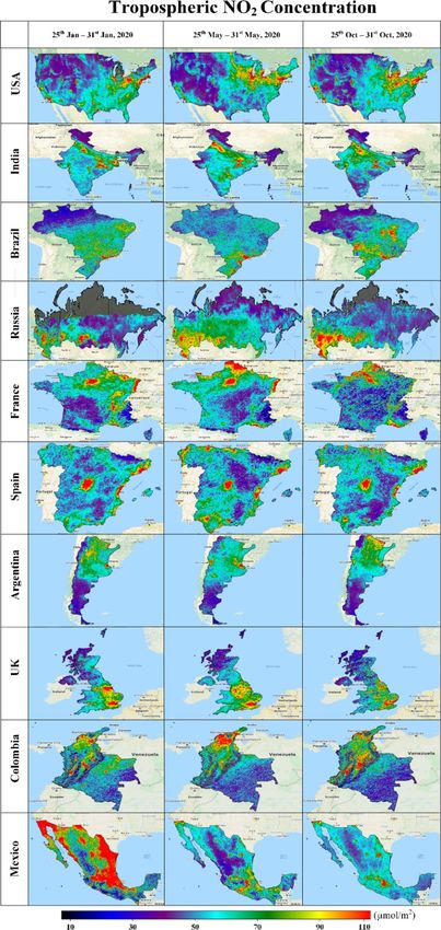
www.nature.com/scientificreports/
harms a wide range of living biological organisms either directly or indirectly21–24. With the rapid growth of
metropolitan areas, particularly in developing countries, considerations of air quality are increasing importance
and air quality monitoring has become a critical challenge25,26.
Local climatic and environmental conditions and variations can play an important role in the transmission
of respiratory diseases, including COVID-19, and exacerbate the risk of morbidity and m ortality26–30. Several
recent studies30–40 has reported correlations between air pollutants like P
M10, PM2.5, CO, N
O2 and O 3 and mortal-
ity rates associated with COVID-19. Taking the example of Northern Italy, which features some of the highest
levels of air pollution in Europe, this region has been highly affected by COVID-19 with high incidence and
mortality rates41. Similarly, several Indian megacities, notably Delhi and Mumbai, which are epicenters of the
coronavirus disease, count amongst the world’s most polluted c ities40–44. Local observations confirm that risks
from respiratory diseases tend to worsen in the winter when air pollution peaks. In this regard, air pollution as a
factor cannot be neglected when considering the transmission and mortality rates related to COVID-19. Hence,
the availability of detailed, spatial information on air pollutants may be important planning tools for mitigating
the impact of the COVID-19 pandemic.
Remote sensing techniques are essential tools for mapping air pollutants especially CO, NO2, SO2, aerosols
and O3. Since these quantities interact dynamically within the atmosphere, wide coverage remote sensing systems
with frequent revisits play a key role. One such system is the Moderate Resolution Imaging Spectroradiometer
(MODIS), whose sensors have contributed to a large number of studies on atmospheric p ollutants45. A newer
source of remotely sensed (satellite-based) information is the Sentinel-5 Precursor (5P), which allows end-users
to obtain information on trace gases such as methane and carbon monoxide on a daily b asis46–48. As indicated
above, air pollution is largely sourced from activities associated with urban environments (including industrial
production) and agriculture where, in particular, the former has been extensively i nvestigated49,50.
In this paper, we explore the dynamics of different air pollutants and qualitatively highlight potential links
with COVID-19 pressures during different phases of the pandemic for ten of the most affected countries in
the world: USA, India, Brazil, Russia, France, Spain, Argentina, UK, Colombia and Mexico. In this respect, we
essentially extend the study by (Mohammad et al)51, who introduce a similar methodology as means of discuss-
ing whether COVID-19 is a “blessing in disguise” based on (visual) observations of a single pollutant (NO2)
with case examples from China, France, Spain, Italy, and USA. Here, we consider five pollutants (CO, NO2,
SO2, aerosols and O3) instead of one and, as just mentioned, ten countries, including also countries in South
America, Russia and India. One could easily argue (and rightly so) that more sophisticated methods, machine
learning, etc. could be used to yield more detailed quantitative results. However, since the intended benefit of
our study lies in extended coverage, in the following we chose to adopt an illustrative methodology similar to
that of (Mohammad et al)51.
Geospatial data was extracted from the European Commission’s Copernicus Earth Observation Satellite
Sentinel-5P. The TROPO spheric Monitoring Instrument (TROPOMI) onboard Sentinel-5P senses air quality
parameters, i.e., methane, aerosols, carbon monoxide, nitrogen dioxide, and sulphur dioxide in the lowest layer
of the atmosphere (troposphere). Spatially distributed information for prominent pollutants, including CO,
NO2, SO2, aerosols and O 3, were acquired for three time periods, which conceptually corresponded to different
seasonal conditions (e.g., winter, summer, autumn), different phases of the COVID-19 pandemic and also to
different levels of mitigating measures. Phase-1 (initial spread of COVID-19) covered the period from 25 Janu-
ary to 31 January 2020; Phase-2 (first wave, extensive lockdowns were implemented in many countries) to the
period from 25 May to 31 May 2020); and Phase-3 (second wave of the pandemic, less restrictive interventions)
to the period from 25 October to 31 October 2020. The observed levels of air pollution are compared with daily
COVID-19 data collected by the Johns Hopkins Corona Virus Resource Center (https://coronavirus.jhu.edu/)
and the Government of India, (www.mygov.in).
Methodology
COVID‑19 data. In general, spatially distributed data on COVID-19 transmission in very high resolution,
i.e., at sub-national, state, regional or even city scales are not freely available, and so in the following, we consider
only aggregated information at the national level. We collected information on cumulative and active infections
and deaths from 22 January 2020 to 10 November 2020, in USA, India, Brazil, Russia, France, Spain, Argentina,
UK, Colombia and Mexico from the Johns Hopkins Corona Virus Resource Center (https://coronavirus.jhu.
edu/) and the Government of India, (www.mygov.in). For the periods 21 May 2020 to 4 June 2020, and 21 Octo-
ber 2020 to 4 November 2020, corresponding to the above-mentioned Phase-2 and Phase-3, we calculated four
indicators, which represent the local state of the COVID-19 pandemic in the ten different countries (Table 1).
The length of these periods are slightly longer than the periods used for extracting the remotely sensed data to
better account for the daily statistical variations in COVID-19 numbers:
• New actives per day: the number of total active COVID-19 cases found for the first and last four days in
the time window are averaged, then subtracted, and finally the average daily change in the number of active
cases is calculated.
• Mean no. active cases: the average number of total active COVID-19 cases during the 15 days.
• New deaths per day: the number of total deaths due to COVID-19 cases found for the first and last four
days in the time window are averaged, then subtracted, and finally the average daily change in the number
of deaths due to COVID-19 is calculated.
• Death % of no. actives: ‘New deaths per day’ as a fraction of the ‘Mean no. active cases’.
Scientific Reports | (2021) 11:8363 | https://doi.org/10.1038/s41598-021-87877-6 2
Vol:.(1234567890)
www.nature.com/scientificreports/
Date 21 May–4 June 2020 (Phase-2) 21 October–4 November 2020 (Phase-3)
New actives per Mean no. active New deaths per Death % of no. New actives per Mean no. active New deaths per Death % of no.
Country day cases day actives day cases day actives
USA − 933 1,120,335 724 0.065 38,354 5,137,198 601 0.012
India 2189 87,248 145 0.166 − 9918 611,118 387 0.063
Brazil 7535 234,560 701 0.299 − 20,217 487,911 288 0.059
Russia 512 227,337 120 0.053 3792 358,719 217 0.061
Colombia 390 17,636 22 0.127 421 71,706 135 0.189
Spain 327 59,780 33 0.055 13,966 948,960 139 0.015
Argentina 348 9737 25 0.256 − 1147 164,598 248 0.151
France 79 90,111 44 0.049 30,680 1,129,328 230 0.020
Mexico 237 14,615 262 1.790 360 151,961 297 0.196
UK 923 215,157 159 0.074 16,102 897,270 179 0.020
Table 1. Indicators of the state of the COVID-19 pandemic in ten selected countries in Phase-2 and Phase-3.
The indicators are based on 15-days of recorded data (number of active infections, the total number of deaths)
provided by the Johns Hopkins Corona Virus Resource Center (https://coronavirus.jhu.edu/).
As shown in Table 1 only the USA experienced a significant temporary decline in the COVID-19 transmis-
sion rate during Phase-2 (Northern Hemisphere Spring), a picture which is reversed in Phase-3. In Phase-3
(Northern Hemisphere Autumn), a significant decline is experienced in India, Brazil, and Argentina, whereas in
Colombia and Mexico just north of the equator the daily transmission rate is almost unchanged from late May
to late October (even though the total number of active cases grows by up to a factor of 10).
Sentinel‑5P based datasets. Sentinel-5P based datasets, including the Aerosol Absorbing Index (AAI),
Carbon Monoxide Column Density, Tropospheric NO2 Concentration, Ozone Total Atmospheric Column and
Sulphur Dioxide Column Density, were extracted from (https://code.earthengine.google.com/) andused for
monitoring the air quality of the ten countries mentioned above. Sentinel-5P uses the TROPOMI instrument,
which has a multispectral sensor that records reflectance of wavelengths optimum for measuring the atmos-
pheric concentration of gases at a spatial resolution of 0.01 arc degree. The retrieval of Sentinel-5P data, its
pre-processing and map generation werecarried out using the Google Earth E ngine52, which is a cloud-based
platform widely used for processing satellite data.
To illustrate the spatio-temporal variation of different air pollutants, the abovementioned quantities were
obtained for three different periods as listed above, corresponding to the initial phase of the COVID-19 pan-
demic, the mid-2020 situation (first phase of the disease) and a late-2020 situation (second or in some cases even
the third phase of the disease):
• Phase-1 (25 January 2020 to 31 January 2020).
• Phase-2 (25 May 2020 to 31 May 2020).
• Phase-3 (25 October 2020 to 31 October 2020).
For comparison, we also extracted comparable data for similar periods in 2019.
Indicators of air pollution. The Aerosol Index Product provided by Sentinel-5P is a qualitative index
that measures the presence of aerosols with substantial absorption. Mathematically, the aerosol index can be
expressed by:
Rmeas ( 2 )Rcalc 1, ALER ( 1 )
Rmeas ( 2 )
AAI = 100 log10 − 100 log10
(1)
Rmeas ( 1 ) Rmeas ( 1 )Rcalc 2, ALER ( 2 )
where AAI is the aerosol absorbing index; R meas depicts measured reflectance at wavelengths λ1 and λ2; Rcalc
describes calculated reflectance from the atmosphere with Rayleigh scattering; A LER is the Lambert equivalent
reflectivity, which is the measured reflectance for wavelength λ2.
The Carbon Monoxide Product is used to estimate the total column that needs to be retrieved—not only
for background CO abundance but also for surface reflection. A physics-based retrieval approach was usedto
derivethe scattering properties of the observed atmosphere and associated trace g ases53,54.
Nitrogen dioxide ( NO2) and nitrogen oxide (NO) referred together as nitrogen oxides are significant trace
gases that are the end products of anthropogenic sources as well as natural processes.
Ozone profiles were utilized to monitor the development of stratospheric ozone. Two types of products were
used; the first covered the entire atmosphere and was derived in the spectral range of 270–320 nm. The second
one covered the tropospheric profile, spanning the spectral range from 300 to 320 nm.
A Slant Column Density (SCD) is derived using the log ratio of the observed UV–visible spectrum, back-
scattered radiation from the atmosphere and the observed spectrum. The SCD depicts the gas concentration,
Scientific Reports | (2021) 11:8363 | https://doi.org/10.1038/s41598-021-87877-6 3
Vol.:(0123456789)
www.nature.com/scientificreports/
which is bias-corrected and converted into vertical columns through air mass factors. The vertical columns are
evaluated mathematically by
Ns − Nsback
Nv = (2)
M
where Nv and Ns respectively represent the vertical and slant column density; Nsback depicts values for background
correction, and M is the air mass factor.
Results and discussion
COVID‑19 pressures. As shown in Table 1, in all of the ten countries the number of active COVID-19
cases increased from late May to late October, ranging from a 50% increase in Russia to a multiplier of 16–17
times in the case of Spain and Argentina. Except for USA and Brazil, the average daily number of deaths due
to COVID-19 also increased, indicating a steeper trajectory, although in relative terms the mortality rate of the
disease, measured as the number of daily deaths divided by the total number of active infections, in most cases
decreased. All of these numbers of course mask out very large (spatial) variations. Hence, transmission rates of
COVID-19 and thereby total numbers of infections are high in densely populated urban areas, where also air
pollution is generally a major challenge. Five of the ten countries depicted here, which currently ranks amongst
those countries in the world most affected by COVID-19: USA, India, Russia, Brazil and UK are also amongst
those with the worst quality of air (see below). On this background, it is reasonable to hypothesize that the
previously documented relationship31–40 between (poor) air quality and the severity of respiratory diseases also
affect the risk of morbidities and mortalities related to COVID-19. A formal attribution of this effect is however
beyond the scope of the current study.
Spatiotemporal distribution of air pollutants. Time-series data of AAI, CO, O3, SO2 and N O2 were
extracted for the three phases, corresponding to the last week of January (outbreak of COVID-19), May (main
lockdown period), and October (normalized situation or partial lockdown). In general, the geographical reparti-
tion of CO, O3, SO2 and N
O2 values delineate a set of characteristic pollution patterns for the USA, European and
Asian countries, which changed between phases.
AAI is a qualitative index indicating the presence of elevated layers of aerosols. Figure 1 indicates significant
absorption for all of the countries in this study: USA, India, Brazil, Russia, France, Spain, Argentina, UK, Colom-
bia, and Mexico. Desert dust, biomass burning and volcanic ash plumes are likely to be the main contributors
to the AAI and can be derived over clear as well as (partly) cloudy pixels. In Fig. 1, large AAI is generally found
for the northern parts and west of the central part of Russia, USA, India, UK, Colombia, Mexico and Spain due
to desert dust and anthropogenic pollution. The AAI over the western and eastern coasts of the USA can also
be attributed to anthropogenic sources, as those regions are the main industrialized areas in the country. States
in the USA dominated by agricultural sectors like the Midwest are generally dominated by lower values of the
AAI. Industrial emissions in South America are also assumed to be important contributors to the global aerosol
production. Overall, the spatial patterns appear to be similar for all retrievals; while small differences in the
retrievals (e.g. varying pixel intensities) may be due to seasonal variations, they could also be explained by other
factors including aerosol model assumptions, sensor calibration and cloud screening. Inter-annual variability
of smoke intensities in the south of the USA and Brazil regions are closely tied to the drought cycle. Meanwhile,
aerosol amounts over India, Brazil, Russia, France, Spain, Argentina, UK, Colombia and Mexico sites are mostly
dominated by the smoke generated from fires associated with savanna and forest clearing practices.
Comparing the spatial distribution of the AAI across all three phases (Phase-1 to Phase-3), unchanged (or
slightly intensified) patterns were principally found for Mexico and Colombia. This suggests that there has been
no significant change in the environmental air quality amid the restrictions installed by the Colombian and
Mexican Governments since March 2020. Conversely, in other countries, the imposed restrictions caused by
lockdowns (Phase-2) appear to have had a positive impact with respect to aerosols, which would be a favorable
condition for COVID-19 mitigation.
Analogous trends are depicted in Figs. 2 and 3 (S1, S2 in the Supplementary Material), indicating improve-
ments in air quality with respect to several of the indicated trace elements, i.e., as a side effect of measures
introduced to mitigate the spread of COVID-19 from March to June 2020. For all countries, the level of CO
generally decreased though with significant spatial variation (Figure S1). NO2 levels also decreased generally in
some countries during Phase-2 (Fig. 2). Conversely, e.g., in India, USA and Russia, regional concentrations of
NO2 and O 3 (Figure S2) increased significantly, in some case by more than 50% during the “lockdown” Phase-2
as compared to Phase-1.
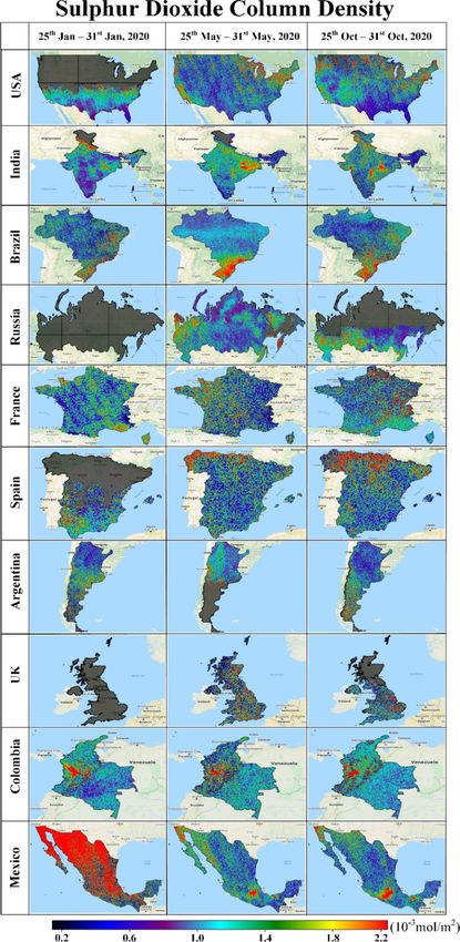
In terms of nitrogen and sulphur dioxide pollutants (Fig. 3), very significant improvements in air quality are
seen in Mexico. At the time of the first reported COVID-19 cases in Mexico (Phase-1), levels of atmospheric
nitrogen and sulphur dioxide pollutants were extremely high, especially in the regions of Baja California in the
West and the North and Eastern regions, including Coahuila, Nuevo Leon and Tamaulipas. Shortly after the
restriction was imposed, NO2 and SO2 amounts declined, suggesting that recorded morbidities and mortalities
due to COVID-19 in Mexico would be less affected by these aspects of air quality.
Comparing the results found for Phase-2 and Phase-3 (Figs. 1, 2, 3, S1, S2), it is evident that the observed
reductions in air pollution levels resulting from the (partial) lockdowns were only temporary. Not accounting
for seasonal variations, as global and national economic activities resumed, levels of air pollution started to rise
again from May to October (e.g., Phase-3).
Scientific Reports | (2021) 11:8363 | https://doi.org/10.1038/s41598-021-87877-6 4
Vol:.(1234567890)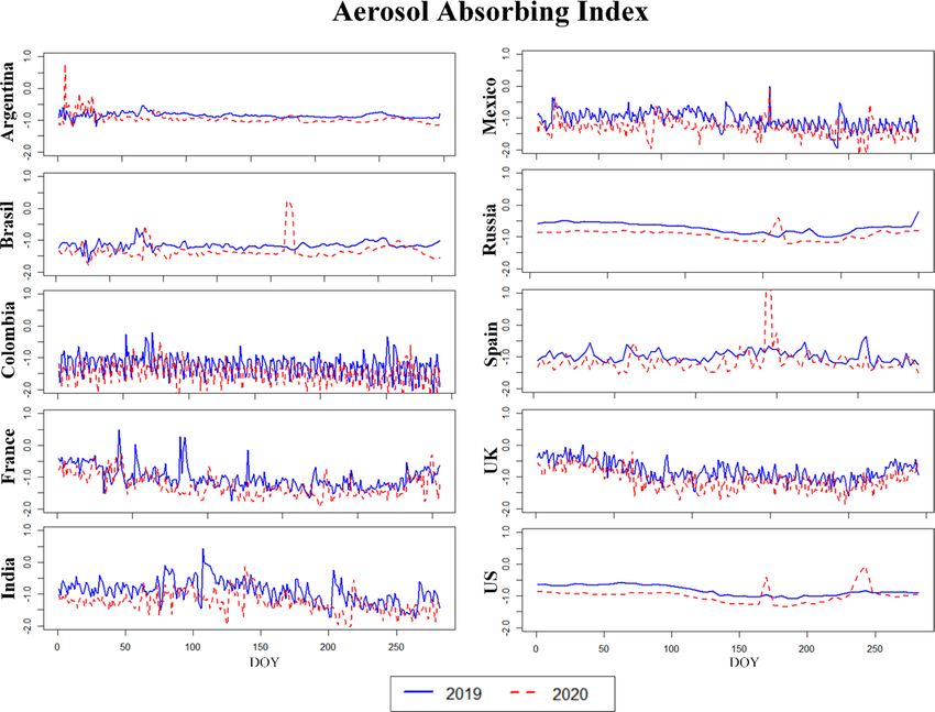
www.nature.com/scientificreports/
Figure 1. Aerosol absorbing index of the top ten most affected countries32.
Temporal dynamics of CO, O3, SO2 and NO2 between 2019 and 2020. Figures 4, 5, 6 (and S3, S4 in
the Supplementary Material) illustrate the temporal (daily) dynamics and seasonal variability of the same set of
Scientific Reports | (2021) 11:8363 | https://doi.org/10.1038/s41598-021-87877-6 5
Vol.:(0123456789)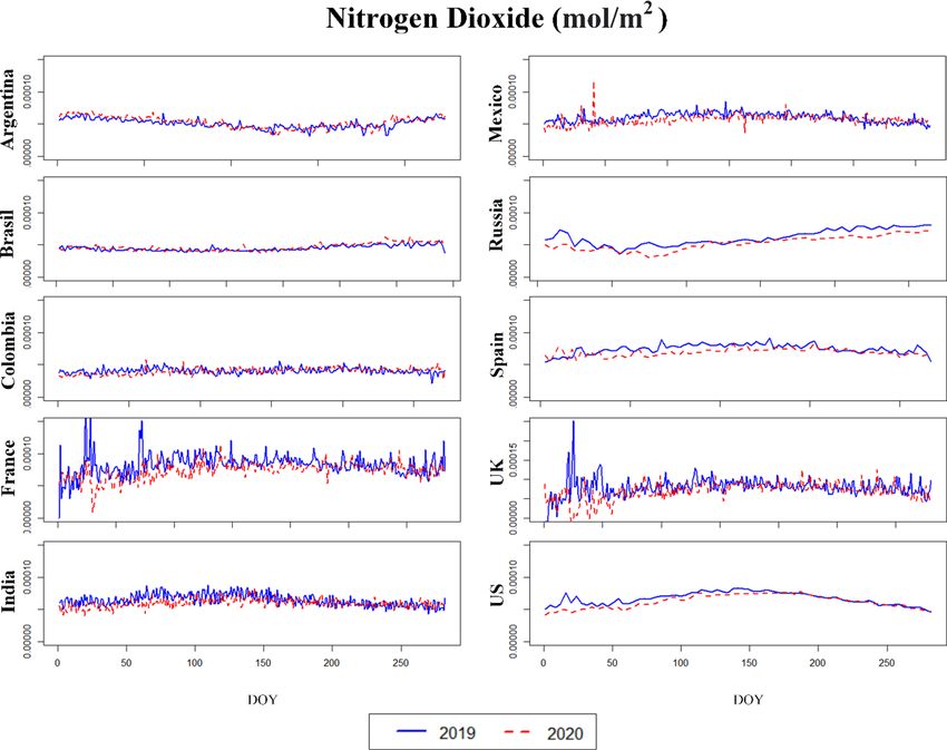
www.nature.com/scientificreports/
Figure 2. Tropospheric nitrogen dioxide concentration of top ten most affected countries36.
pollutants (aerosols, CO, O
3, SO2 and NO2) as depicted on Figs. 1, 2, 3. The blue curves correspond to data from
2019 whereas the red curves indicate data for 2020. The mid-points of the three phases studied above correspond
Scientific Reports | (2021) 11:8363 | https://doi.org/10.1038/s41598-021-87877-6 6
Vol:.(1234567890)www.nature.com/scientificreports/
Figure 3. The sulphur dioxide column density of the top ten most affected countries36.
Scientific Reports | (2021) 11:8363 | https://doi.org/10.1038/s41598-021-87877-6 7
Vol.:(0123456789)www.nature.com/scientificreports/
Figure 4. Aerosol absorbing index (AAI) of the countries for the years 2019 and 2020. DOY day of the year.
to the following days-of-year (DOY): 28 (28 January 2020), 149 (28 May 2020) and 302 (28 October 2020). Both
of the time series (2019, 2020) are truncated after Phase 3 (Figs. 4, 5, 6, S3 and S4).
Assuming 2019 to be a “normal year”, we generally find that the seasonal variations in 2020 are preserved
for all variables despite the modifications brought about by the implementation of COVID-19 policies, includ-
ing lockdowns. For the developing countries Mexico and Colombia, a highly fluctuating AAI is observed both
in 2019 and in 2020 (Fig. 4), which is probably not related to COVID-19 but due to some other cause like the
frequent biomass burning for energy purposes in the countryside.
As already mentioned, net reductions in CO, O3, NO2 and SO2 were observed for many countries in 2020—
particularly when going towards May 2020. These reduction scans are attributed to the complete or partial
lockdown of industrial activities and vehicle traffic across the American, Asian and European continents. To
exemplify, by population, Europe ranks third among regions of the world with 9.8% of the total population in
the world living in Europe (Worldometer’s 2020 statistics). Over 70% of the European population, however,
lives in urban areas, explaining the generally high levels of CO, O3, SO2 and N O2 pollution. By the end of May
2020, multiple European cities that previously featured high levels of air pollution (CO, O 3, NO2 and SO2) now
reported very low pollution levels, indicating improvements in air quality. Comparing 2019 and 2020 (Fig. 5),
the tropospheric N O2 column number density maintained high values of about 0.0001 mol/m2 for the USA,
France and UK. In countries like Argentina, Brazil, Colombia, Russia, and Spain the equivalent numbers were
found to be lower (closer to below 0.0001 mol/m2 in 2019) and improving during the principal 2020 lockdown.
For several major cities in France, Spain, UK, USA and Russia, O 3 concentrations increased in 2019 compared
to previous years (Figure S4). They slightly decreased in 2020 especially during the lockdown (e.g., Phase-2)
(0.16 mol/m2) (Figure S4). In the Latin American countries, represented by Columbia, Brazil, Argentina and
Mexico, O3 concentrations were comparably found to be lower (0.12 and 0.14 mol/m2 respectively) than the
just mentioned countries. This is in line with the fact that many lower-income countries emit significantly lower
levels of atmospheric pollutants. Finally, for S O2 France and the USA recorded a high level of concentration
(~ 0.002 mol/m2) (Fig. 6), although we also note that the spatial distribution of SO2 pollutants is influenced by
local factors in almost all cases.
Several authors have already demonstrated a correlation between air pollution and morbidity and mortality
linked to respiratory diseases and in particular to COVID-19. Given the different scope and (coarse) resolution
of the COVID-19 data used, it was however not possible to carry out a similar attribution within this study. In a
qualitative sense, it is evident though that the relatively moderate health and multi-sectorial impacts suffered in
the Spring of 2020 (compared to the present situation worldwide) may have taken advantage of the significantly
lower levels of select air pollutants that was a welcome but unexpected side effect of the lockdowns introduced
Scientific Reports | (2021) 11:8363 | https://doi.org/10.1038/s41598-021-87877-6 8
Vol:.(1234567890)www.nature.com/scientificreports/
Figure 5. Nitrogen dioxide of the countries for the years 2019 and 2020.
in many countries. For example, this could prospectively help to explain the positive situation in the USA in late
May 2020, which only a few months later was turned upside down. Conversely, our results also seem to indicate
that seasonal variations alone are insufficient as a means of explaining the potential variation in the risk of,
e.g., mortalities due to COVID-19. That said, as already suggested by our analysis, air pollution—especially in
cities—tend to reach a high point in the winter season. When combined with the current (and very alarming)
growth in the incidence rates of COVID-19 all over the world, this could exacerbate the already very critical
situation in many countries, where COVID-19 threatens the capacity of national and local health systems. This
could for example be true in developing countries like India, where 21 out of 30 major cities are listed among
the most polluted cities in the world.
Conclusion
In this study, we explore the utility of remotely sensed data as a means of qualitatively explaining the observed
developments of the COVID-19 pandemic, and in particular, the varying risk of a deadly outcome. On this
background, data from Sentinel-5P was retrieved for 2019 and 2020. For 2020, three conceptual phases of the
diseases were investigated: an early stage at the end of January (Phase-1), a stage a least partly overlapping the
extensive lockdown, which was demanded in many countries, starting from around March (Phase-2); and finally,
a stage in late October, where lockdowns had been relaxed, leading to resumed local and global economic activi-
ties (Phase-3).
Using data extracted from the Johns Hopkins Corona Virus Resource Center, we illustrate the temporal
development of the novel coronavirus in ten of the most severely affected countries in the world. From Phase-2 to
Phase-3, the globally accumulated numbers of COVID-19 infections have increased dramatically with the USA in
the less fortunate role of being first on the list. For India, Brazil and Argentina, a decline in the number in active
infections is observed, for Columbia and Mexico the numbers are largely unchanged, whereas for the remaining
countries (USA, Russia, France, Spain and the UK) the development follows the increasing global trend.
Comparing different indicators of air pollution for 2019 and 2020, despite the anomalous modifications
introduced by the lockdowns, seasonal variations were generally found to be unchanged, and indicating that
observed variations in COVID-19 conditions are likely to be linked to air quality. Further, the level of most
pollutants temporarily declined in Phase-2. On this background, our study confirms that air pollution may be a
good predictor for the local and national severity of COVID-19 infections.
Scientific Reports | (2021) 11:8363 | https://doi.org/10.1038/s41598-021-87877-6 9
Vol.:(0123456789)www.nature.com/scientificreports/
Figure 6. Sulphur dioxide column density of the countries for the years 2019 and 2020. DOY day of the year.
Data availability
Data on COVID-19 was acquired from the repositories of the Johns Hopkins Corona Virus Resource Center,
the Worldometer and the Ministry of Health and Family Welfare, Government of India. These data sources are
freely accessible through web-based archives.
Received: 14 September 2020; Accepted: 6 April 2021
References
1. Kuniya, T. Prediction of the epidemic peak of coronavirus disease in Japan. J. Clin. Med. 9, (2020).
2. Linton, N. M. et al. Incubation period and other epidemiological characteristics of 2019 novel coronavirus infections with right
truncation: A statistical analysis of publicly available case data. J. Clin. Med. 9, 538 (2020).
3. Jung, S.-M. et al. Real-time estimation of the risk of death from novel coronavirus (COVID-19) infection: Inference using exported
cases. J. Clin. Med. 9, 523 (2020).
4. Doornik, J.A., Castle, J.L. & Hendry, D.F. Short-term forecasting of the coronavirus pandemic, Int. J. Forecast. (2020). https://doi.
org/10.1016/j.ijforecast.2020.09.003.
5. Ioannidis, J.P.A., Cripps, S. & Tanner, M.A. Forecasting for COVID-19 has failed. Int. J. Forecast. (2020).https://doi.org/10.1016/j.
ijforecast.2020.08.004.
6. Lead better, M.R. On a basis for ’Peaks over threshold’ modeling, statistics & probability. Letters 12, 357–362 (1991).
7. Nikolopoulos, K., Punia, S., Schäfers, A., Tsinopoulos, C. & Vasilakis, C. Forecasting andplanning during a pandemic: COVID-19
growth rates, supply chain disruptions, and governmental decisions. Eur. J. Oper. Res. 290, 99–115 (2020).
8. Nikolopoulos, K. We need to talk about intermittent demand forecasting. Eur. J. Oper. Res. https://doi.org/10.1016/j.ejor.2019.12.
046 (2020).
9. Al-Shammari, A. A. A. et al. Real-time tracking and forecasting of the COVID-19 outbreak in Kuwait: A mathematical modeling
study. MedRxiv 05(03), 20089771. https://doi.org/10.1101/2020.05.03.20089771 (2020).
10. Doornik, J.A., Castle, J.L., Hendry, D.F. Short-term forecasting of the coronavirus pandemic. Int. J. Forecast. (2020). https://doi.
org/10.1016/j.ijforecast.2020.09.003.
11. Petropoulos, F., Makridakis, S. Forecasting the novel coronavirus COVID-19. PLOS ONE 15(3), e0231236 (2020).
12. IHME COVID-19 health service utilization forecasting, Murray, C.J. Forecasting the impact of the first wave of the COVID-19
pandemic on hospital demand and deaths for the USA and European Economic Area countries. MedRxiv(2020b). https://doi.org/
10.1101/2020.04.21.20074732.
13. Hopkins, J. CSSEGIS and Data/ COVID-19: noval coronavirus global cases. https://gisanddata.maps.arcgis.com/apps/opsdashboa
rd (2020).
Scientific Reports | (2021) 11:8363 | https://doi.org/10.1038/s41598-021-87877-6 10
Vol:.(1234567890)www.nature.com/scientificreports/
14. Nikolopoulos, K., Goodwin, P., Patelis, A. & Assimakopoulos, V. Forecasting with cue information: a comparison of multiple
regression with alternative forecasting approaches. Eur. J. Oper. Res. 180, 354–368 (2007).
15. Petropoulos, F., Makridakis, S. & Stylianou, N. COVID-19: Forecasting confirmed cases and deaths with a simple time-series
model. Int. J. Forecast. (2020).doi: https://doi.org/10.1016/j.ijforecast.2020.11.010 .
16. Pinson, P. & Makridakis, S. Pandemics and forecasting: The way forward through the Taleb-Ioannidis debate. Int. J. Forecast.
forthcoming (2020).
17. Pranab, C. et al. The 2019 novel coronavirus disease (COVID-19) pandemic: A review of the current evidence. Indian J. Med. Res.
151, 147–159 (2020).
18. Gupta, A., Bherwani, H., Gautam, S., Anjum, S., Musugu, K., Kumar, N., Anshul, A., & Kumar, R. Air pollution aggravating
COVID-19 lethality? Exploration in Asian cities using statistical models. Environ. Dev. Sustain. 1–10 (2020).
19. Singh, R. K. et al. Prediction of the COVID-19 pandemic for the top 15 affected countries: Advanced autoregressive integrated
moving average (ARIMA) model. JMIR Public Health Surveill 6, e19115 (2020).
20. Yang, Z. et al. Modified SEIR and AI prediction of the epidemics trend of COVID-19 in China under public health interventions.
J. Thorac. Dis. 12, 165–174 (2020).
21. Gautam, S. & Hens, L. COVID-19: impact by and on the environment, health and economy. Environ. Dev. Sustain. 22, 4953–4954
(2020).
22. Pirouz, B., Shaffiee Haghshenas, S., Shaffiee Haghshenas, S. & Piro, P. Investigating a serious challenge in the sustainable develop-
ment process: Analysis of confirmed cases of COVID-19 (new type of coronavirus) through a binary classification using artificial
intelligence and regression analysis. Sustainability 12, 2427 (2020).
23. Zou, L. et al. SARS-CoV-2 viral load in upper respiratory specimens of infected patients. N. Engl. J. Med. 382, 1177–1179 (2020).
24. Nsoesie, E., Mararthe, M. & Brownstein, J. Forecasting peaks of seasonal influenza epidemics. PLoS Curr 5, (2013).
25. Petropoulos, F. & Makridakis, S. Forecasting the novel coronavirus COVID-19. PLoS ONE 15, e0231236 (2020).
26. Nayeem, A., Hossai̇n, M., Majumder, A. & Carter, W. Spatiotemporal Variation of Brick Kilns and it’s relation to Ground-level
PM2.5 through MODIS Image at Dhaka District, Bangladesh. Int. J. Environ. Pollut. Environ. Model. 2, 277–284 (2019).
27. Han, C. & Hong, Y.-C. Decrease in ambient fine particulate matter during COVID-19 crisis and corresponding health benefits in
Seoul, Korea. Int. J. Environ. Res. Public Health 17, 5279 (2020).
28. Azuma, K., Kagi, N., Kim, H. & Hayashi, M. Impact of climate and ambient air pollution on the epidemic growth during COVID-
19 outbreak in Japan. Environ. Res. 190, 110042 (2020).
29. Manoj, M. G., Kumar, M. S., Valsaraj, K. T., Sivan, C. & Vijayan, S. K. Potential link between compromised air quality and trans-
mission of the novel corona virus (SARS-CoV-2) in affected areas. Environ. Res. 190, 110001 (2020).
30. Conticini, E., Frediani, B., & Caro, D. Can atmospheric pollution be considered a co-factor in extremely high level of SARS-CoV-2
lethality in Northern Italy? Environ. Pollut. 114465, (2020).
31. Yongjian, Z., Jingu, X., Fengming, H. & Liqing, C. Association between short-term exposure to air pollution and COVID-19
infection: Evidence from China. Sci. Total Environ. 727, 138704 (2020).
32. Tobías, A. et al. Changes in air quality during the lockdown in Barcelona (Spain) one month into the SARSCoV-2 epidemic. Sci.
Total Environ. 726, 138540 (2020).
33. Mahato, Susanta, Swades Pal& Krishna Gopal Ghosh. Effect of lockdown amid COVID-19 pandemic on air quality of the megacity
Delhi, India. Science of the Total Environment 730, 139086 (2020).
34. Rui, B. & Zhang, A. Does lockdown reduce air pollution? Evidence from 44 cities in northern China. Sci. Total Environ. 731, 139052
(2020).
35. Sharma, S., Zhang, M., Gao, J., Zhang, H. & Kota, S. H. Effect of restricted emissions during COVID-19 on air quality in India.
Sci. Total Environ. 728, 138878 (2020).
36. Kanniah, K. D., Zaman, N. A. F. K., Kaskaoutis, D. G. & Latif, M. T. COVID-19’s impact on the atmospheric environment in the
Southeast Asia region. Sci. Total Environ. 736, 139658 (2020).
37. Otmani, A. et al. Impact of Covid-19 lockdown on PM10, S O2 and NO2 concentrations in Salé City (Morocco). Sci. Total Environ.
735, 139541 (2020).
38. Selvam, S. et al. SARS-CoV-2 pandemic lockdown: Effects on air quality in the industrialized Gujarat state of India. Sci. Total
Environ. 737, 140391 (2020).
39. Kumari, Pratima& Durga Toshniwal. Impact of lockdown measures during COVID-19 on air quality–A case study of India. Int.
J. Environ. Health Res. 1–8 (2020).
40. Wang, L., Li, M., Yu, S., Chen, X., Li, Z., Zhang, Y., Jiang, L., Xia, Y., Li, J., Liu, W. & Li, P. Unexpected rise of ozone in urban and
rural areas, and sulfur dioxide in rural areas during the coronavirus city lockdown in Hangzhou, China: Implications for air quality.
Environ. Chem. Lett. 1–11 (2020).
41. Masum, M. H. & Pal, S. K. Statistical evaluation of selected air quality parameters influenced by COVID-19 lockdown. Global J.
Environ. Sci. Manag. 6, 85–94 (2020).
42. Filippini, T. et al. Satellite-detected tropospheric nitrogen dioxide and spread of SARS-CoV-2 infection in Northern Italy. Sci. Total
Environ. 739, 140278 (2020).
43. Karuppasamy, M.B., Seshachalam, S., Natesan, U., Ayyamperumal, R., Karuppannan, S., Gopalakrishnan, G. & Nazir, N. Air pol-
lution improvement and mortality rate during COVID-19 pandemic in India: global intersectional study. Air Qual. Atmos. Health
1–10 (2020).
44. Singh, V. et al. Diurnal & temporal changes in air pollution during COVID-19 strict lockdown over different regions of India.
Environ. Pollut. 266, 115368 (2020).
45. Misra, P., Fujikawa, A. & Takeuchi, W. Novel decomposition scheme for characterizing urban air quality with MODIS. Remote
Sens. 9, 812 (2017).
46. Mahato Susanta & Krishna Gopal Ghosh. Short-term exposure to ambient air quality of the most polluted Indian cities due to
lockdown amid SARS-CoV-2. Environ. Res. 188, 109835 (2020).
47. Pacheco, H. et al. NO2 levels after the COVID-19 lockdown in Ecuador: A trade-off between environment and human health.
Urban Clim. 34, 100674 (2020).
48. Urrutia-Pereira, M., Mello-da-Silva, C. A. & Solé, D. COVID-19 and air pollution: A dangerous association?. Allergol. Immuno-
pathol. 48, 496–499 (2020).
49. Duncan, B.N., Prados, A.I., Lamsal, L.N., Liu, Y., Streets, D.G., Gupta, P., Hilsenrath, E., Kahn, R.A., Nielsen, J.E., Beyersdorf, A.J.
& Burton, S.P. Satellite data of atmospheric pollution for U.S. air quality applications: Examples of applications, summary of data
end-user resources, answers to FAQs, and common mistakes to avoid. Atmos. Environ. 94, 647–662 (2014).
50. Gelper, S., Fried, R. & Croux, C. Robust forecasting with exponential and Holt-Winters smoothing. J. Forecast. 29, 285–300 (2010).
51. Muhammad, S., Long, X. & Salman, M. COVID-19 pandemic and environmental pollution: A blessing in disguise?. Sci. Total
Environ. 728, 138820 (2020).
52. Gorelick, N. et al. Google earth engine: Planetary-scale geospatial analysis for everyone. Remote Sens. Environ. 202, 18–27 (2017).
53. He, G., Pan, Y., Tanaka, T. COVID-19, city lockdowns, and air pollution: evidence from China (2020). medRxiv https://doi.org/
10.1101/2020.03.29.20046649.
54. Liu, F., Page, A., Strode, S.A., Yoshida, Y., Choi, S., Zheng, B., Lamsal, L.N., Li, C., Krotkov, N.A., Eskes, H., van der, A.R. Abrupt
declines in tropospheric nitrogen dioxide over China after the outbreak of COVID-19. arXiv preprint arXiv:2004.06542 (2020).
Scientific Reports | (2021) 11:8363 | https://doi.org/10.1038/s41598-021-87877-6 11
Vol.:(0123456789)www.nature.com/scientificreports/
Author contributions
P.K., M.D. and R.K.S.: writing-draft, modeling, software. P.K.S., M.K.P. and A.A.: modeling, software. S.S.S.,
A.K.P., M.D, M.K.: supervision, Data analysis. M.D., M.R, B.H.T.: revision, writing-review. M.D.S.: supervision,
funding acquisition.
Funding
The authors acknowledge financial support from the Spanish Government, Grant RTI2018- 354 094336-B-I00
(MCIU/AEI/FEDER, UE), the Spanish Carlos III Health Institute, COV 20/01213, and the Basque Government,
Grant IT1207-19.
Competing interests
The authors declare no competing interests.
Additional information
Supplementary Information The online version contains supplementary material available at https://doi.org/
10.1038/s41598-021-87877-6.
Correspondence and requests for materials should be addressed to P.K.
Reprints and permissions information is available at www.nature.com/reprints.
Publisher’s note Springer Nature remains neutral with regard to jurisdictional claims in published maps and
institutional affiliations.
Open Access This article is licensed under a Creative Commons Attribution 4.0 International
License, which permits use, sharing, adaptation, distribution and reproduction in any medium or
format, as long as you give appropriate credit to the original author(s) and the source, provide a link to the
Creative Commons licence, and indicate if changes were made. The images or other third party material in this
article are included in the article’s Creative Commons licence, unless indicated otherwise in a credit line to the
material. If material is not included in the article’s Creative Commons licence and your intended use is not
permitted by statutory regulation or exceeds the permitted use, you will need to obtain permission directly from
the copyright holder. To view a copy of this licence, visit http://creativecommons.org/licenses/by/4.0/.
© The Author(s) 2021
Scientific Reports | (2021) 11:8363 | https://doi.org/10.1038/s41598-021-87877-6 12
Vol:.(1234567890)You can also read