Impact of dynamic snow density on GlobSnow snow water equivalent retrieval accuracy
←
→
Page content transcription
If your browser does not render page correctly, please read the page content below
The Cryosphere, 15, 2969–2981, 2021
https://doi.org/10.5194/tc-15-2969-2021
© Author(s) 2021. This work is distributed under
the Creative Commons Attribution 4.0 License.

Impact of dynamic snow density on GlobSnow snow water
equivalent retrieval accuracy
Pinja Venäläinen, Kari Luojus, Juha Lemmetyinen, Jouni Pulliainen, Mikko Moisander, and Matias Takala
Finnish Meteorological Institute, P.O. Box 503, 00101 Helsinki, Finland

Correspondence: Pinja Venäläinen (pinja.venalainen@fmi.fi)

Received: 14 January 2021 – Discussion started: 22 January 2021
Revised: 12 April 2021 – Accepted: 26 May 2021 – Published: 28 June 2021

Abstract. Snow water equivalent (SWE) is an important            1   Introduction
variable in describing global seasonal snow cover. Tradition-
ally, SWE has been measured manually at snow transects           Snow water equivalent (SWE) is an important property of the
or using observations from weather stations. However, these      seasonal snow cover, and estimates of SWE are required in
measurements have a poor spatial coverage, and a good al-        many hydrological and climatological applications, includ-
ternative to in situ measurements is to use spaceborne pas-      ing climate model evaluation (Mudryk et al., 2018) and fore-
sive microwave observations, which can provide global cov-       casting freshwater availability. Maximum SWE before the
erage at daily timescales. The reliability and accuracy of       start of spring snowmelt is one of the most important snow
SWE estimates made using spaceborne microwave radiome-           characteristics for run-off and river discharge forecasts (Bar-
ter data can be improved by assimilating radiometer observa-     nett et al., 2005; Barry, 2002).
tions with weather station snow depth observations as done          Snow depth or SWE can be estimated by interpolating sur-
in the GlobSnow SWE retrieval methodology. However, one          face snow depth (Dyer and Mote, 2006) or snowfall measure-
possible source of uncertainty in the GlobSnow SWE re-           ments (Broxton et al., 2016). However, the limited spatial
trieval approach is the constant snow density used in mod-       and temporal coverages of the ground-based measurements,
elling emission of snow. In this paper, three versions of spa-   especially in northern and alpine regions, limit the quality
tially and temporally varying snow density fields were imple-    of estimates (Broxton et al., 2016; Mortimer et al., 2020).
mented using snow transect data from Eurasia and Canada          An alternative approach for estimating SWE is to use satel-
and automated snow observations from the United States.          lite measurements as they can provide global spatial coverage
Snow density fields were used to post-process the baseline       and good temporal resolution.
GlobSnow v.3.0 SWE product. Decadal snow density infor-             Spaceborne passive microwave radiometer (for example
mation, i.e. fields where snow density for each day of the       Chang and Foster, 1987; Kelly et al., 2003; Pulliainen, 2006)
year was taken as the mean calculated for the correspond-        or active radar (for example Lievens et al., 2019; Rott et al.,
ing day over 10 years, was found to produce the best results.    2010) observations can be used for retrieving SWE informa-
Overall, post-processing GlobSnow SWE retrieval with dy-         tion. Passive microwave observations are commonly used as
namic snow density information improved overestimation of        these provide frequent repeat coverage, and the influence of
small SWE values and underestimation of large SWE values,        atmospheric conditions on the observation is limited. Fur-
though underestimation of SWE values larger than 175 mm          thermore, passive microwave radiometer data are also avail-
was still significant.                                           able from 1978 onwards, which allows the analysis of long
                                                                 time series. Many passive microwave radiometer-based ap-
                                                                 proaches for estimating SWE are adopted from an algo-
                                                                 rithm proposed by Chang and Foster (1987) for estimating
                                                                 snow depth from horizontally polarized Scanning Multichan-
                                                                 nel Microwave Radiometer (SMMR) measurements. The al-
                                                                 gorithm is based on the difference in measured brightness

Published by Copernicus Publications on behalf of the European Geosciences Union.
2970                                                P. Venäläinen et al.: Dynamic snow density for GlobSnow SWE retrieval

temperatures at a frequency insensitive to dry snow, around        whole Northern Hemisphere for the whole period of GSv3.0
19 GHz, and at a frequency sensitive to dry snow, around           SWE data record, 1979–2018.
37 GHz. The uncertainty of SWE retrievals based on the ra-
diometer measurements alone can be quite high (Mudryk et
al., 2015). Retrieval algorithms that use only radiometer data     2     Data and methods
tend to underestimate SWE in deep snow conditions (Derk-
                                                                   2.1     Snow density and SWE data
sen et al., 2005), and the performance of these algorithms is
even more limited in wet snow conditions (Armstrong and            2.1.1    Eurasia
Brodzik, 2001).
   To overcome the problems connected to stand-alone pas-          In situ snow density and SWE measurements were used to
sive microwave SWE retrievals, ground-based observations           obtain dynamic snow density fields and validate the results
and satellite radiometer data can be combined as done in the       of SWE retrievals. SWE and density datasets for Eurasia
assimilation approach for SWE retrieval introduced by Pulli-       were obtained from Russia (Bulygina et al., 2011) and Fin-
ainen (2006) and complemented by Takala et al. (2011). This        land (Haberkorn, 2019). These datasets contain snow tran-
assimilation-based approach was used as the baseline method        sect data. Snow transects consist of manual gravimetric snow
for the Global Snow Monitoring for Climate Research (Glob-         measurements made at multiple locations along a pre-defined
Snow) initiative of the European Space Agency (ESA). The           transect several hundreds of metres to several kilometres in
GlobSnow method has been shown to produce good results             length which are averaged together to obtain a single repre-
when compared to typical stand-alone radiometer algorithms         sentative (in regard to the spatial resolution of utilized pas-
(Mortimer et al., 2020). The GlobSnow version 3.0 (GSv3.0)         sive microwave radiometers) SWE value for a given transect
climate data record with spatial bias correction was used for      on a given date.
accurate reconstruction of the Northern Hemisphere snow               Russian data, from a substantial network of snow tran-
mass and its trends for period of 1979–2018 (Pulliainen et         sects, has been made available via the All-Russia Research
al., 2020). Improving the GlobSnow SWE retrieval method-           Institute of Hydrometeorological Information-World Data
ology will help to further enhance our understanding of the        Centre (RIHMI-WDC) website. This Russian snow survey
Northern Hemisphere snow conditions and their changes.             dataset contains data from routine snow surveys operated
   The GlobSnow SWE retrieval utilizes a fixed density of          at 515 meteorological station locations, and data are avail-
240 kg m−3 throughout the retrieval regardless of the snow         able from 1966 to 2020 (Bulygina et al., 2011); data from
depth, location, or time of the year (Takala et al., 2011),        1979 to 2018 are used in this study. Routine snow surveys
which is a known source of uncertainty in the retrieval. The       are run through the cold season every 10 d or every 5 d dur-
density of snow changes with time and place, and it is greatly     ing the intense snowmelt season. The Finnish Environment
affected by surrounding weather conditions. For example,           Institute (SYKE) has a network of about 160 snow survey
wind breaks down snow crystals, both on the ground and             courses that have been operated from the beginning of the
falling from the sky, which allows snow crystals to pack to-       20th century (Haberkorn, 2019). These 2 to 4 km long snow
gether tightly and increases the density of snow (Jordan et al.,   survey courses that go through different landscapes are vis-
1999). The age of the snow cover also affects its density as       ited monthly, and 80 snow depth measurements are made
the snow on the ground is constantly undergoing metamor-           along the snow course through varying landscapes about
phism (Maurice and Harold, 1981).                                  50 m apart. Eight snow density and SWE measurements are
   One approach considered for GlobSnow SWE retrieval              made along each snow course. An aggregate of the SWE
methodology for estimating temporally and spatially varying        measurements is applied to describe the SWE conditions for
snow densities was to use a statistical snow density model         the snow course for the given sampling date.
presented by Sturm et al. (2010), which predicts density of           The Russian snow transect dataset was divided into two
snow as a function of the snow depth, day of the year, and         parts. The division of data was done by finding the nearest
snow class (Luojus et al., 2013b). However, applying den-          neighbours and separating them into different datasets. The
sities obtained using this approach did not improve retrieval      first part of the data were used for implementing the dynamic
skill notably (Luojus et al., 2013a). A different approach for     snow density maps, and the second part, together with snow
obtaining varying snow density information is to use avail-        transect data from Finland, was used for validating snow
able snow density data to create snow density fields by ap-        density and SWE results. The implementation dataset con-
plying temporal and spatial interpolation.                         tains 257 locations, and the validation data are formed from
   In this study, dynamic snow density information obtained        data from 625 locations. Implementation and validation snow
from ground measurements using interpolation is used to            transect locations are shown in Fig. 1. Figure 2 shows his-
post-process the GSv3.0 SWE climate data record. Three dif-        tograms of the implementation and validation snow density
ferent versions of the snow densities are implemented for          values.
Eurasia for the years 2000 to 2009. Additionally, one version
of the dynamic snow densities is also implemented for the

The Cryosphere, 15, 2969–2981, 2021                                                   https://doi.org/10.5194/tc-15-2969-2021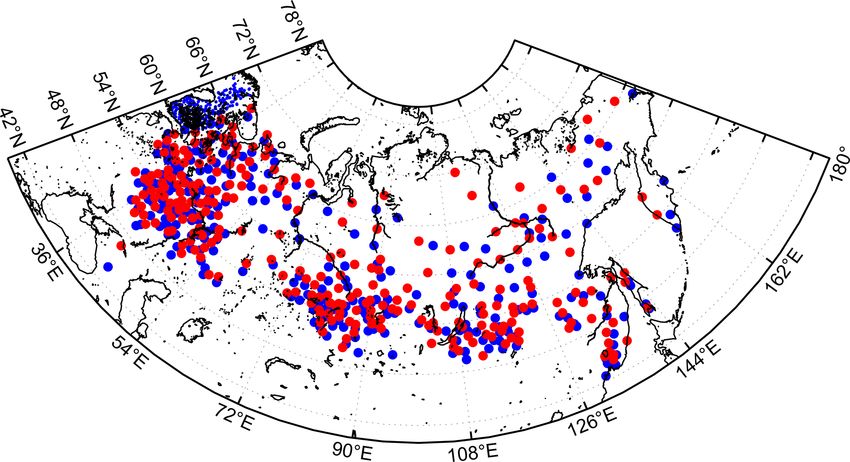
P. Venäläinen et al.: Dynamic snow density for GlobSnow SWE retrieval 2971
Figure 3. Average snow density and SWE versus DOW for snow
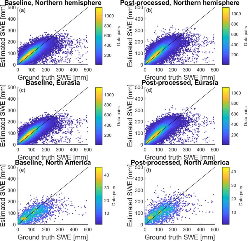
Figure 1. Locations of Eurasian snow courses divided into two sets:
transect in western Russia with latitude 59.4◦ N and longitude
implementation (red) and validation (blue).
33.1◦ E using multi-decadal data. Blue asterisks show average den-
sity calculated for each DOW separately. Red square markers show
average densities calculated using data for two consecutive days if
available. The red dashed line shows averaged SWE for the same
location.
1000 kg m−3 . These measurements are most likely erroneous
as snow densities typically range between 50 and 550 kg m−3
(Fierz et al., 2009). After filtering, average snow density val-
ues were calculated for each DOW that had at least one mea-
surement.
Most density measurements have been done systemati-
cally on the same DOW from year to year, with few excep-
tions. This difference in measurement days may cause aver-
age densities to fluctuate from one day to another as some
density values are not averages but measurements from one
specific year. To avoid these fluctuations in multi-decadal
and decadal versions, if two consecutive DOWs had mea-
Figure 2. Histogram of the implementation and validation densities surements, the average density is calculated using data from
for Eurasia for 2000–2009. both days, and this density was assigned the DOW value of
the first day. Outlier data points were removed from multi-
decadal and decadal datasets after averaged densities were
We divided the Eurasian snow density implementation calculated. Outliers were determined to be data points that
dataset into three distinct ways to create three different ver- differ from two previous and two following points by more
sions of dynamic snow density maps. For the first version, than 50 kg m−3 . Figure 3 shows how average densities cal-
called the multi-decadal version, all data between 1979 and culated for each DOW and non-consecutive DOWs differ for
2018 were used. The second version, called the decadal ver- one snow transect location for the multi-decadal dataset. The
sion, uses data from 2000 to 2009. The third version, called depicted snow transect is located in western Russia. Figure 3
the annual version, uses data from 2000 to 2009 and pro- also shows the 40-year average SWE for each DOW for the
duces daily density maps for each year using only data from same station.
the year under investigation.
A day-of-the-winter (DOW) value was added to each snow 2.1.2 North America
density measurement. DOW values are a modification of
the day-of-the-year (DOY) values. DOW values start from The North American dataset consists of data from Canada
1 September and then continue to grow from there until the and the United States. The Canadian snow course network is
last day of August. This means that 1 January has a DOW sampled twice per month (around the first and 15th) during
value of 123, and 30 August has a value of 365 or 366. the snow season, and the dataset extends from 1981–2016
They are used because the Northern Hemisphere winter sea- (Brown et al., 2019). The Canadian dataset was comple-
son spans from September until June over the new year. mented with snow observations from 443 SNOTEL stations
The Eurasian snow survey data were filtered to remove all located in Alaska and the north-western United States (Ser-
negative density observations and all observations larger than reze et al., 1999). Data from southern states are not included
https://doi.org/10.5194/tc-15-2969-2021 The Cryosphere, 15, 2969–2981, 2021
2972                                                P. Venäläinen et al.: Dynamic snow density for GlobSnow SWE retrieval

                                                                   snow depth measurements are also used to form a continu-
                                                                   ous background field of snow depth independently from pas-
                                                                   sive microwave measurements. The interpolated snow depth
                                                                   field is fused with space-borne brightness temperature obser-
                                                                   vations, using the scene brightness temperature model in a
                                                                   Bayesian approach that weights all information sources with
                                                                   their estimated variances, to provide the final SWE estimates.
                                                                   A constant value of snow density is used (240 kg m−3 ).
                                                                      The retrieval method does not produce SWE estimates for
                                                                   mountainous areas, glaciers, or Greenland. The data record
                                                                   is based on data from the SMMR aboard NIMBUS-7, SSM/I
                                                                   and SSMIS sensors on board DMSP 5D F-series satellites,
Figure 4. Locations of North American snow measurements di-        and synoptic weather station snow depth data from the North-
vided into two sets: implementation (red) and validation (blue).   ern Hemisphere.

                                                                   2.3   Creation of snow density fields
as most of the snow in these areas is in mountains which
                                                                   Two main steps for generating snow density fields are tem-
are excluded from the retrieval. The SNOTEL dataset differs
                                                                   poral and spatial interpolation. Snow density measurements
from the Canadian and Eurasian datasets, as it consists of
                                                                   are made usually every 10 or 15 d, and thus, there are many
automated daily measurements instead of manual snow tran-
                                                                   days without snow density observations. Simple linear inter-
sect measurements. SNOTEL stations collect data on snow-
                                                                   polation was used to obtain estimates of snow density values
pack SWE, snow depth, precipitation, and air temperature.
                                                                   for the days lacking observations.
SWE is measured by a snow pillow filled with an antifreeze
                                                                      The length of the snow season depends on the year and
solution. Hourly data are available from the snow pillows,
                                                                   place, but to get similar series for each station, and for each
but daily measurements were used as they are more robust as
                                                                   version, the average of three first existing densities was added
hourly data are easily affected by wind and sensor issues.
                                                                   to DOW 30 if a station did not have measurements from
   A small part of North American data were separated to be
                                                                   DOW 30 or before this day. Similarly, if the station did not
used for validation of results. The implementation set con-
                                                                   have any measurement after DOW 280, the average of the
tains 1455 locations, and the validation set is made from 242
                                                                   last three densities was calculated and added as the density
locations. The locations that form the validation and imple-
                                                                   for DOW 280. After this procedure, all stations have density
mentation datasets are shown in Fig. 4.
                                                                   values from DOW 30 to DOW 280, and interpolation could
2.2    Baseline SWE retrieval                                      be performed for this period. Figure 5 shows the results of in-
                                                                   terpolation for all three versions for one snow transect loca-
The European Space Agency (ESA) GlobSnow and succeed-              tion. The interpolation of the multi-decadal dataset produces
ing projects have produced a family of daily satellite-based       the smoothest results, and yearly data show the most fluctua-
SWE climate data records spanning over 40 years. The most          tion.
recent GSv3.0 data record is based on methodology intro-              We used ordinary kriging interpolation for interpolating
duced in Pulliainen (2006) and Takala et al. (2011), and the       snow density values for areas without observations. Krig-
latest version is presented in detail in Luojus et al. (2021).     ing interpolation is a spatial interpolation method that pre-
The retrieval algorithm combines satellite-based passive mi-       dicts values for the location with no measurements based on
crowave measurements with ground-based synoptic weather            the spatial autocorrelation of measured values (Goovaerts,
station snow depth observations by Bayesian non-linear iter-       1997). This means that two closely located points are more
ative assimilation.                                                likely to have similar values than two points further afield.
   The GlobSnow approach uses two vertically polarized             The main advantages of kriging interpolation compared to
brightness temperature observations at 19 and 37 GHz and           nongeostatistical interpolation methods are that kriging in-
a scene brightness temperature model (the HUT snow emis-           terpolation provides variance of predicted values and that
sion model; Pulliainen et al., 1999). First, an effective snow     the spatial smoothing is defined through the variogram. The
grain size is estimated for grid cells that coincide with          model of spatial variability can be expressed as (Høst, 1999)
weather station snow depth observations. The snow grain            Z (s) = µ (s) +  (s) ,                                     (1)
sizes are used to construct a kriging interpolated background
map of the effective grain size, including an estimate of the      where Z (s) denotes the predicted value at some location,
effective grain size error. This spatially continuous map of       µ (s) is the deterministic function describing the trend com-
grain size is then used as an input for HUT model inversion        ponent of Z (s), and  (s) is the stochastic locally varying but
to provide an estimate of SWE. The daily weather station           spatially dependent residuals.

The Cryosphere, 15, 2969–2981, 2021                                                   https://doi.org/10.5194/tc-15-2969-2021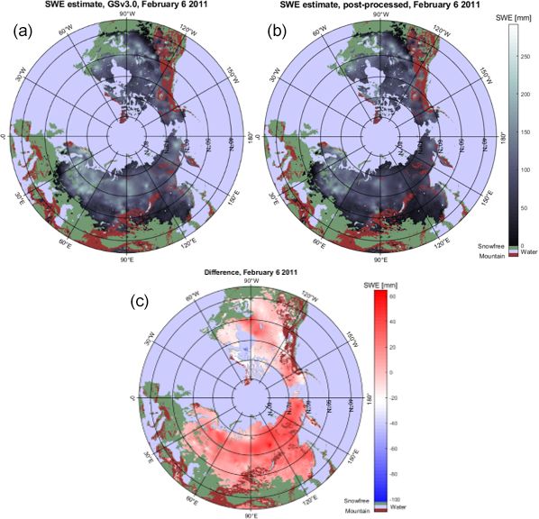
P. Venäläinen et al.: Dynamic snow density for GlobSnow SWE retrieval                                                                     2973

                                                                          Table 1. Summary of calculated validation parameters for three
                                                                          snow density sets for the years 2000–2009.

                                                                                                   Bias     RMSE          MAE     Correlation
                                                                                              [kg m−3 ]   [kg m−3 ]   [kg m−3 ]    coefficient
                                                                              Multi-decadal        2.7        48.4        35.8           0.71
                                                                              Decadal              0.9        48.8        35.8           0.71
                                                                              Annual              −2.2        45.0        32.3           0.76

                                                                          2.4     Usage of snow density information and validation

                                                                          The derived snow density information is used to post-process
                                                                          the baseline GSv3.0 SWE retrieval. Post processing of SWE
                                                                          retrieval means that SWE values obtained are scaled with the
                                                                          ratio of dynamic and constant snow density:
                                                                                                ρdynamic
Figure 5. Temporally interpolated densities for snow transects in         SWEnew = SWE ·                  ,                                 (5)
                                                                                                ρconstant
north central Russia for multi-decadal and decadal versions. The
figure also shows results of interpolation for 2 years of annual inter-
                                                                          where ρconstant has values of 240 kg m−3 . Scaling is per-
polation, 2004 and 2008.
                                                                          formed for each pixel within the area for which dynamic
                                                                          densities are available. For the regions outside dynamic snow
  The spatial autocorrelation is modelled with a semivari-                density information, the constant density consideration is re-
ogram (Goovaerts, 1997):                                                  tained.
                                                                             The obtained snow densities and post-processed SWE
2γ (d) = Var (Z (si ) − Z (si + d)) ,                              (2)    datasets were validated using independent validation data.
                                                                          Validation locations were separated from the data used for
with the assumption of intrinsic stationarity (variance on the            generating snow density fields to ensure independent cross-
right-hand side is only dependent on the vector difference d)             validation. Root-mean-squared error (RMSE), bias, correla-
and the assumption that the process is isotropic (the autocor-            tion coefficients, and mean absolute error (MAE) are the four
relation is only dependent on the distance between observa-               statistical measures used for assessing the performance.
tions). The empirical semivariogram can be estimated from
the observations as follows (O’Sullivan and Unwin, 2010):
                                                                          3     Results
              Nd
        1 X
γ̂ d̃j =         E (Z (si ) − Z (si + d)) , ∀d ∈ d̃j ,             (3)    3.1     Eurasia 2000–2009
         2Nd i=1

where Z (si ) and Z (si + d) are sampled data pairs at distance           3.1.1     Snow density
d, and d̃j is the distance between observations. In this study,
                                                                          Annual, decadal, and multi-decadal versions of snow density
an exponential function is used for the variogram:
                                                                          fields were produced for Eurasia for the years 2000–2009.
γ (d) = c1 · exp (d · c2 ) + c0 .                                  (4)    These three versions of dynamic snow densities were com-
                                                                          pared to validation snow density data from Eurasia over the
Snow density values were predicted for each pixel in 25 km                same 10-year period. A summary of the validation is shown
Equal Area Scalable Grid (EASE-Grid version1, to match                    in Table 1. Figure 6 shows the comparison of estimated
GSv3 processor grid) between latitudes from 42 to 80◦ N and               and observed densities at validation sites for multi-decadal,
for longitudes from 20 to 180◦ E. The snow density values                 decadal, and annual snow densities. As Fig. 2 shows, most
were estimated using coordinates for centres of each pixel.               snow density values range between 150 and 350 kg m−3 ,
Density maps were made for all three versions of snow den-                which can explain the departure from 1 : 1 fit for small and
sities for each day starting from DOW 30 and ending at DOW                large snow density values seen in Fig. 6.
280. Pixels that are not on land are assigned a value of −1,                 Multi-decadal and decadal versions of snow densities ex-
and land areas outside the area of interpolation are desig-               hibit similar behaviour, with the multi-decadal version hav-
nated a constant density of 240 kg m−3 (effectively retaining             ing slightly smaller RMSE and larger correlation coefficient
the original retrieval methodology for those regions where                but larger bias than the decadal version. MAE is equal for
snow density could not be reliably established).                          these two versions. The annual version differs from the other

https://doi.org/10.5194/tc-15-2969-2021                                                            The Cryosphere, 15, 2969–2981, 2021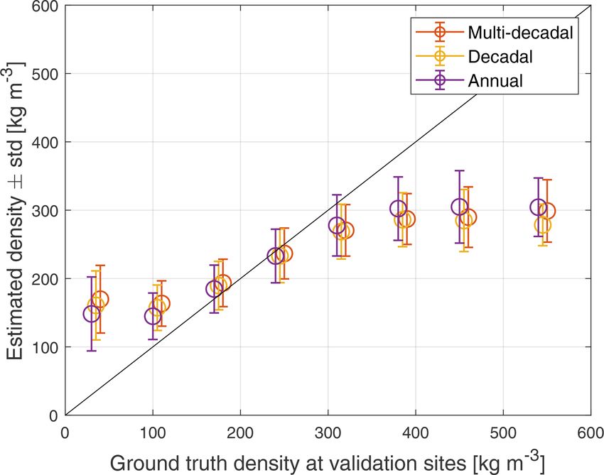
2974                                                 P. Venäläinen et al.: Dynamic snow density for GlobSnow SWE retrieval

                                                                     Figure 7. The mean error for the baseline, multi-decadal, decadal,
                                                                     and annual SWE estimates, 2000–2009 Eurasia.

Figure 6. Comparison of multi-decadal, decadal, and annual density
estimates. As can be observed, annual densities perform best for
                                                                     present in the baseline retrieval, though the improvements are
small and large density values.
                                                                     smaller than the improvements for small SWE values.
                                                                        Post-processing with the annual densities produces worse
                                                                     results than the other two post-processed versions when SWE
two versions more, and it estimates snow densities below             values up to 500 mm are considered. The worse behaviour of
200 and above 300 kg m−3 better than the other versions.             the annual densities for larger SWE values can be caused by
The multi-decadal and decadal versions of snow densities             the annual density dataset having a larger range of densities
are produced from data that are averaged from a large num-           than the other two density datasets. If SWE estimation has
ber of measurements. This averaging means that the highest           been close to correct, but the density used in the retrieval is
and lowest measurements have a diminished effect on esti-            far from the estimated density, post-processing causes SWE
mated snow densities. Annual densities have a wider range            estimation to change significantly. A wider range of densi-
of densities present in the data used for deriving these dy-         ties causes more significant changes in the post-processing.
namic densities compared to the range of densities used for          Annual and multi-decadal density sets had higher estimates
deriving the other two sets of the density maps. Annual den-         for large densities than decadal densities, which explains the
sities also have a negative bias, while the other two versions       positive mean error for SWE estimates higher than 150 mm.
have positive biases.
                                                                     3.2   Northern Hemisphere, 1979–2018
3.1.2   Post-processed SWE
                                                                     Based on the results obtained for the years 2000–2009, the
The three different density sets were used to post-process           decadal version of snow densities was extended to cover the
the baseline GSv3.0 SWE data between 2000 and 2009. Ob-              whole Northern Hemisphere and the whole period of the
tained SWE values were compared to validation SWE mea-               baseline retrieval. Four separate sets of density maps were
surements of the Eurasian dataset. Two validations were per-         made, each covering 1 decade starting from the 1980s and
formed: the first validation took into account SWE values up         ending in the 2010s. The decadal density maps were calcu-
to 500 mm, and the second validation considered SWE val-             lated using static 10-year periods not running 10-year aver-
ues only up to 150 mm, as the bulk of the observations are           ages because these two methods were found to produce very
below this value. Table 2 summarizes the results of the SWE          similar results, and producing four set of maps is consider-
validation (for different snow density realizations). Figure 7       ably simpler than producing separate maps for every year us-
shows mean errors for the baseline, multi-decadal, decadal,          ing moving 10-year averages. The density maps were made
and annual versions.                                                 using the methods explained in Sect. 2, with a few excep-
   Post-processing the baseline product with any of the three        tions: (1) the spatial interpolation was performed for latitudes
density sets improves the baseline product. For SWE val-             from 35 to 80◦ N and for longitudes from 180◦ W to 180◦ E
ues up 130 mm, all three post-processed datasets show sim-           to cover the same area as the baseline retrieval, and (2) the
ilar behaviour, and as Fig. 7 shows, the overestimation of           North American dataset was filtered before adding DOW val-
SWE values between 0 and 100 mm present in the base-                 ues. Filtering consisted of two steps. First, locations that were
line retrieval has been mitigated with post-processing. Post-        within the same EASE grid cell were combined, and the aver-
processing also improves the underestimation of large values         age value of measurements was calculated for each day. Then

The Cryosphere, 15, 2969–2981, 2021                                                      https://doi.org/10.5194/tc-15-2969-2021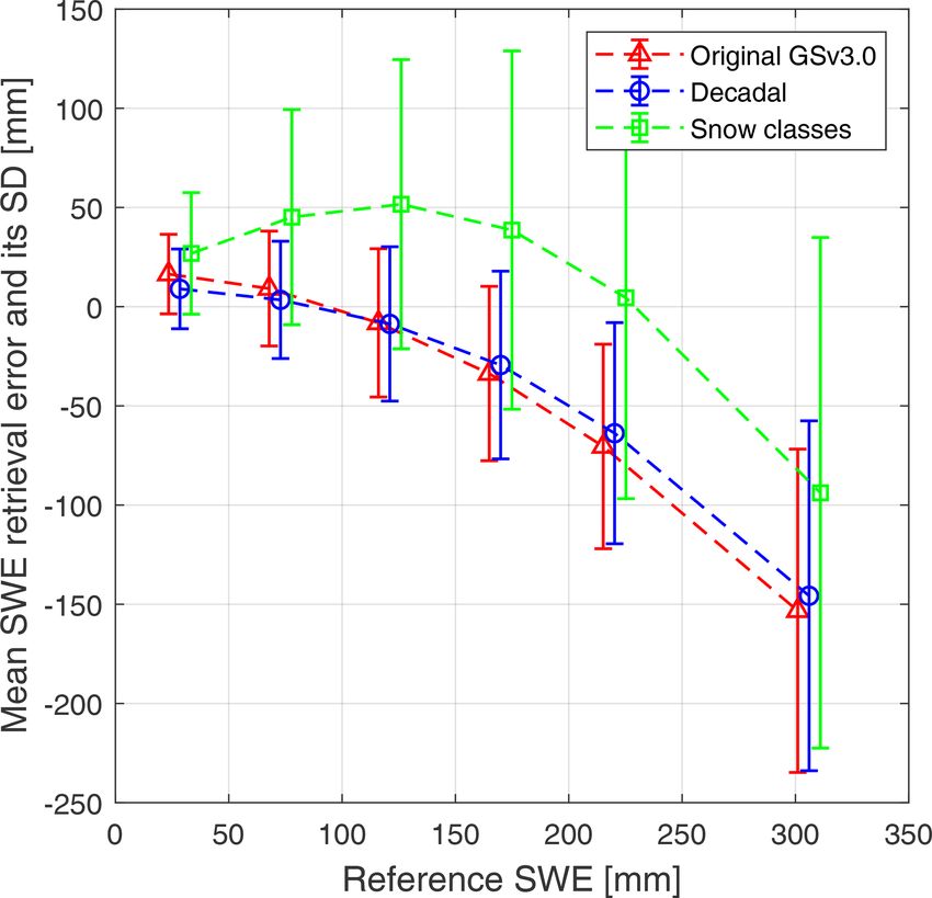
P. Venäläinen et al.: Dynamic snow density for GlobSnow SWE retrieval                                                                 2975

Table 2. Results of validation for different Eurasian datasets for the years 2000–2009; left values are for SWE < 500 mm and bold values are
for SWE < 150 mm.

                                                                 Bias     RMSE           MAE      Correlation
                                                                [mm]       [mm]          [mm]      coefficient
                               GlobSnow v3.0 (Eurasia)     2.9/10.0     39.5/29.7    27.2/23.2      0.73/0.74
                               Multi−decadal               −1.0/4.6     37.7/28.0    23.9/20.0      0.77/0.77
                               Decadal                     −2.5/3.2     37.4/27.5    23.6/19.5      0.77/0.77
                               Annual                      −2.2/3.7     38.5/27.5    23.9/19.6      0.77/0.78

Table 3. Results of validation for the whole Northern Hemisphere, Eurasia, and North America for the whole winter, February, April, and
December for 1979–2018. Left values are for SWE < 500 mm and bold values are for SWE < 150 mm.

                  Area            Period       Product                     Bias        RMSE          MAE         Correlation
                                                                          [mm]          [mm]         [mm]         coefficient
                                  Winter       GSv3.0                  1.2/9.7       43.5/31.6   29.3/24.5         0.70/0.71
                                               post-processed        −1.4/5.4        42.5/30.8   27.0/22.0         0.73/0.73
                                  December     GSv3.0                14.6/16.1       29.5/25.8   21.8/20.8         0.68/0.75
                  Northern                     Post-processed          0.1/1.7       24.3/18.5   14.7/13.4         0.69/0.75
                  Hemisphere      February     GSv3.0                11.1/16.8       36.9/30.6   26.6/24.3         0.75/0.77
                                               Post-processed         5.2/11.2       36.4/28.6   24.6/21.4         0.74/0.76
                                  April        GSv3.0             −32.7/−17.4        63.9/40.8   43.8/31.3         0.68/0.61
                                               Post-processed      −20.5/−9.5        61.1/42.4   41.8/32.3         0.68/0.61
                                  Winter       GSv3.0               −19.7/3.3        70.9/42.7   48.2/33.1         0.50/0.48
                                               post-processed       −16.0/4.8        69.9/45.6   47.4/34.1         0.53/0.48
                                  December     GSv3.0                14.8/18.3       41.2/36.6   30.2/27.6         0.51/0.48
                  North                        Post-processed         6.0/10.3       38.4/31.0   26.2/23.1         0.48/0.51
                  America         February     GSv3.0               −0.7/14.7        51.4/37.3   36.7/29.7         0.67/0.63
                                               Post-processed       −2.4/12.5        52.9/39.0   37.2/29.7         0.65/0.60
                                  April        GSv3.0             −75.2/−36.9       110.8/60.7   83.0/48.9         0.40/0.32
                                               Post-processed     −60.2/−25.2       105.0/62.3   77.8/49.7         0.40/0.32
                                  Winter       GSv3.0                 2.5/10.0       41.2/30.8   28.2/24.0         0.73/0.72
                                               post-processed        −0.5/5.5        40.2/29.8   25.8/21.4         0.75/0.75
                                  December     GSv3.0                11.0/12.4       29.5/26.1   22.0/21.1         0.67/0.72
                  Eurasia                      Post-processed          0.0/1.5       23.9/18.1   14.5/13.1         0.70/0.76
                                  February     GSv3.0                10.5/15.5       36.5/30.9   26.5/24.5         0.75/0.76
                                               Post-processed         5.6/11.1       35.5/28.1   24.0/21.1         0.74/0.76
                                  April        GSv3.0             −30.2/−16.8        59.6/39.6   42.3/30.4         0.72/0.64
                                               Post-processed      −18.3/−8.8        57.6/41.4   39.8/31.5         0.71/0.63

a mountain mask was applied to remove locations in moun-                   The RMSE was 43.5 and 42.5 mm for the baseline retrieval
tainous areas. After these filtering steps, the North American          and retrieval post-processed with decadal densities, respec-
implementation set contained 869 locations, and the valida-             tively. Figure 8 shows scatter plots for the whole Northern
tion set was made from 201 locations.                                   Hemisphere for the baseline (Fig. 8a) and the post-processed
   These new decadal snow density maps were used to post-               datasets (Fig. 8b), and as expected, post-processing reduces
process the whole GSv3.0 baseline dataset and the results ob-           overestimation of SWE values between 10 and 100 mm. Fig-
tained were compared to validation datasets from Eurasia and            ure 8 also shows density scatter plots for the baseline and the
North America. Again, SWE values up to 500 and 150 mm                   post-processed datasets for Eurasia (Fig. 8c, d) and North
were validated separately. Validation was performed for the             America (Fig. 8e, f). The post-processed Eurasian dataset
whole winter (September to June) and separately for Febru-              shows similar improvements as the overall Northern Hemi-
ary, April, and December. Table 3 summarizes the results of             sphere dataset; overestimation of SWE values between 10
this evaluation. Table 3 shows results for the whole Northern           and 100 mm has been mitigated. For Eurasia, post-processing
Hemisphere and separately for Eurasia and North America.                improves estimations every month when SWE values up
                                                                        to 500 mm are considered, and the biggest improvement in

https://doi.org/10.5194/tc-15-2969-2021                                                          The Cryosphere, 15, 2969–2981, 2021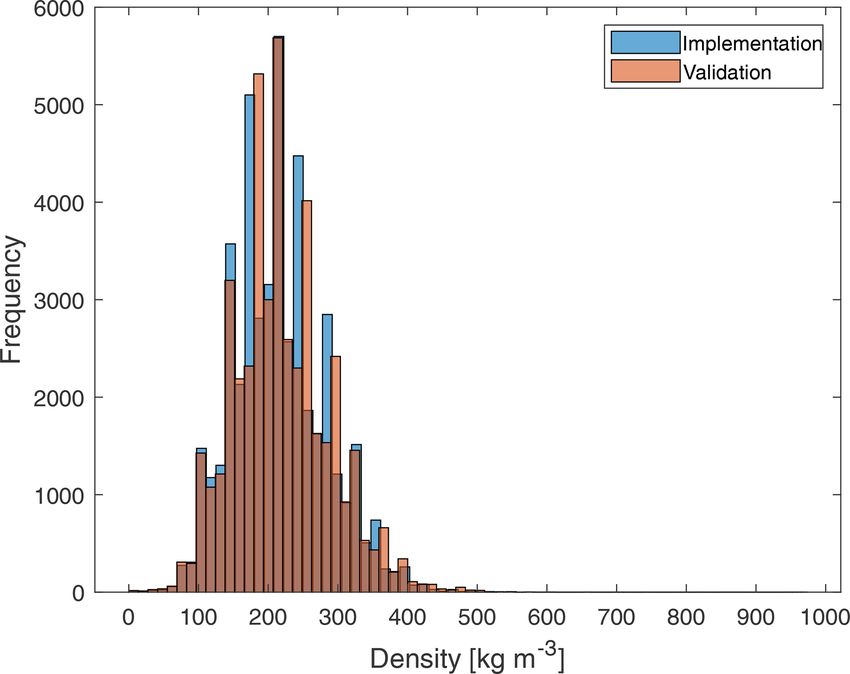
2976                                                 P. Venäläinen et al.: Dynamic snow density for GlobSnow SWE retrieval

Figure 8. Density scatterplots of GSv3.0 baseline and post-processed retrieval accuracy for 1979–2018 for the whole Northern Hemisphere,
Eurasia, and North America.

RMSE happens in December (over 5 mm). When SWE val-                   line minus post-processed). Maps show how SWE values are
ues only up to 150 mm are considered, we see similar big im-          lower in the post-processed maps, and the map of differences
provement in December, but in April baseline retrieval pro-           reveals that post-processing causes bigger changes in Eurasia
duces better results than the post-processed dataset.                 than in North America.
   North American datasets also show some improvements
but not as clearly as the Eurasian dataset. For North Amer-
ica SWE values are improved for December and April when               4   Discussion
SWE values up to 500 mm are considered. When SWE values
up to 150 mm are considered, improvements are seen only               GlobSnow 3.0 SWE retrieval accuracy is affected by the
in December. Figure 9, which shows the mean retrieval er-             overestimation of small SWE values and underestimation of
ror and standard deviation of the error for baseline and post-        large SWE values. Passive microwave SWE retrievals tend to
processed retrievals for the Northern Hemisphere, Eurasia,            systematically underestimate SWE under deep snow condi-
and North America, agrees with these findings. Mean er-               tions as the snowpack changes from scattering medium to a
rors for North America are similar for SWE values below               source of emission, which becomes significant for SWE re-
100 mm for the baseline and post-processed retrievals, but for        trievals over about 150 mm. While the GlobSnow retrieval
larger values, the mean errors of the post-processed dataset          estimates large SWE values better than stand-alone passive
are smaller than the errors of the baseline set. For Eurasia and      microwave SWE retrieval, errors are still evident for deep
the Northern Hemisphere, the mean error is systematically             snow. The underestimation of SWE in GlobSnow retrieval
smaller for the post-processed dataset than for the baseline          under deep snow conditions is additionally driven by the
dataset. Figure 10 shows SWE maps for 6 February 2011,                constant density that relates snow depth and SWE. The con-
for the baseline and post-processed retrievals. Figure 10 also        stant density tends to decrease SWE estimates for late win-
shows the difference between these two SWE maps (base-                ter when the snowpacks are usually denser than the constant
                                                                      density applied. Post-processing with dynamic densities im-

The Cryosphere, 15, 2969–2981, 2021                                                        https://doi.org/10.5194/tc-15-2969-2021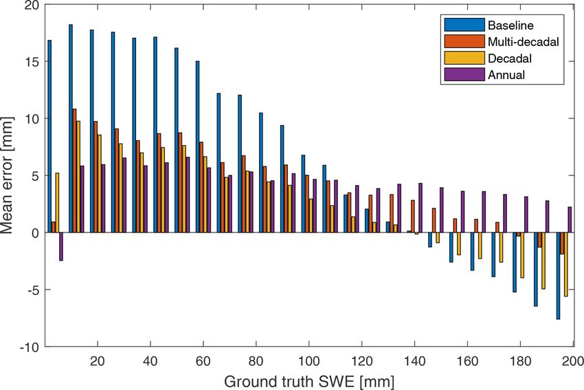
P. Venäläinen et al.: Dynamic snow density for GlobSnow SWE retrieval                                                       2977

Figure 9. Comparisons of the mean error and standard deviations between baseline and post-processed SWE datasets.

proves the overall deep snow retrieval performance as the               Improvements produced by post-processing are more sig-
SWE values are scaled up with larger dynamic snow density.           nificant for Eurasia than for North America. The North
Similarly, the post-processing helps to improve the overesti-        American reference measurements consist of both snow tran-
mation of small SWE values. The constant snow density used           sect and point measurements, which may affect the results.
in the retrieval tends to be too large in the early winter when      The measurement frequency of the daily SNOTEL data also
the snow is fresh, and the density is at its lowest.                 differs from the Eurasian and Canadian data, which have
   Even though the improvements obtained by post-                    measurements from every 10 to 15 d. However, when SNO-
processing for the whole winter are not large (RMSE reduced          TEL data were resampled to 10 d intervals and validation pa-
by about 1 mm), significant improvements are still gained.           rameters were recalculated, no significant differences were
The small changes in the whole dataset are expected, as most         detected. Another possible source of error in the SNOTEL
of the validation data are from areas where there are no large       data is the location of snow depth sensor. In some locations,
mistakes in the baseline product and snow density is close           snow depth is not measured on top of the snow pillow but
to the constant snow density of 240 km m−3 in mid-winter.            next to the pillow, and this may affect the accuracy of the
However, the monthly analyses (Table 3) show that the im-            snow density values. However, it should be noted that the
provements in overestimation of SWE values in early winter           GlobSnow retrieval is known to have worse performance in
(December) are significant: the RMSE is reduced by about 5           Canada, and this is partly due to higher average SWE com-
(7) mm for SWE values up to 500 (150) mm, and bias is re-            pared to Eurasia (Mortimer et al., 2020).
duced by 15 mm for both versions of validation. Figure 7 also           As shown by the results, post-processing with dynamic
shows that significant improvements (5–10 mm smaller mean            snow densities can be used to improve existing datasets, and
error) are obtained with post-processing for SWE < 100 mm            the post-processing procedure is straightforward to perform.
and SWE > 170 mm.                                                    However, implementing dynamic snow densities directly into

https://doi.org/10.5194/tc-15-2969-2021                                                    The Cryosphere, 15, 2969–2981, 2021
2978                                                 P. Venäläinen et al.: Dynamic snow density for GlobSnow SWE retrieval

Figure 10. SWE maps for baseline GSv3.0 retrieval (a), post-processed retrieval (b), and difference between GSv3.0 and post-processed
retrieval (post-processed subtracted from the baseline) for 6 February 2011. The post-processed SWE values are lower as overestimation of
small SWE values is reduced.

the retrieval could possibly produce even more notable im-             final SWE estimation, as well as the accuracy of the individ-
provements and is a key research topic to be studied in the            ual grain size estimates. Similarly, applying a wrong density
future. Snow density is one of the input parameters of the             value in the final retrieval step potentially deteriorates the ac-
HUT snow emission model, determining the absorption co-                curacy of the HUT model and thus retrieval skill.
efficient in snow, refraction, and transmissivity at the air–             Although better results might be achieved with implement-
snow interface and transmissivity at the snow–ground inter-            ing dynamic densities into the retrieval, post-processing is
face through modelled permittivity of the snow layer (Pul-             justified as it can be used to study different implementations
liainen et al., 1999). The HUT model is used for determin-             of the snow densities with relative ease, and the results ob-
ing effective snow grain size over weather station locations           tained with post-processing are similar to results obtained
as well as for obtaining the final SWE estimates using nu-             with implementing dynamic densities in retrieval. Running
meric model inversion (Takala et al., 2011). The final snow            the full retrieval algorithm is very time consuming and as
grain size (and its variance) at each location is the average          such not well suited for testing small changes in methodol-
grain size of the six nearest stations. If the true snow den-          ogy. Post-processing can be used to study which densities
sity between stations significantly changes, the variance of           and methodologies produce the best results, and these densi-
the estimated snow grain sizes increases. This in turn poten-          ties can then be implemented into a final retrieval product.
tially reduces the weight of radiometer measurements on the            Also, as some areas have more snow density information

The Cryosphere, 15, 2969–2981, 2021                                                        https://doi.org/10.5194/tc-15-2969-2021
P. Venäläinen et al.: Dynamic snow density for GlobSnow SWE retrieval                                                           2979

                                                                   polynomial interpolation of averaged values or yearly values,
                                                                   could be evaluated in future investigations.

                                                                   5   Conclusions

                                                                   In this study spatially and temporally changing snow den-
                                                                   sity fields were implemented using snow density measure-
                                                                   ments from Eurasia and North America. The development
                                                                   of dynamic snow density for GlobSnow retrieval was im-
                                                                   plemented as part of the European Space Agency Climate
                                                                   Change Initiative – Snow (Snow CCI) project and will be im-
                                                                   plemented in future SWE retrievals. The dynamic snow den-
                                                                   sity fields were used to post-process GlobSnow version 3.0
                                                                   SWE retrievals. Post-processing was found to improve over-
                                                                   estimation of small SWE values between 10–100 mm and un-
                                                                   derestimation of large SWE values. This indicates that the
                                                                   constant density used in the baseline retrieval is too large for
                                                                   early winter and too small for late winter. The overall results
                                                                   indicate a clear path forward to improve the overall Glob-
Figure 11. Comparisons of the mean error and standard deviations
                                                                   Snow SWE retrieval methodology by application of dynamic
between baseline and datasets post-processed with decadal snow
densities and densities based on fixed snow classes according to   snow density in the post-processing scheme.
Sturm et al. (2010).

                                                                   Code and data availability. The GlobSnow code is available
                                                                   at http://www.globsnow.info/swe/archive_v3.0/source_codes/ (Lu-
available than others, the introduced post-processing meth-        ojus et al., 2020a), and the GlobSnow v3.0 data are available
                                                                   at https://www.globsnow.info/swe/archive_v3.0/L3A_daily_SWE/
ods provide feasible tools to improve the accuracy of the
                                                                   (Luojus et al., 2020b). The snow density processing code is avail-
global GlobSnow-data-based SWE estimates for regional hy-          able upon request from the corresponding author.
drological applications in such areas where snow density in-
formation is available.
   Different approaches for varying snow density for               Author contributions. PV, KL, JL, and JP conceived the concept of
satellite-based SWE retrievals have been used. The AMSR-E          the study. PV performed the analyses, data processing, and com-
v1.0 product (Kelly, 2009) uses spatially varying but tempo-       puting and produced the first draft of the manuscript, which was
rally static snow density maps based on snow classes sug-          subsequently edited by KL, JL, and JP. MT and MM contributed to
gested in Sturm et al. (1995). However, evaluation of this         the analytical tools and methods.
product by Tedesco and Narvekar (2010) pointed out the
need to also have temporal variability in the snow density.
The AMSR-E SWE v2.0 product uses spatially and tempo-              Competing interests. The authors declare that they have no conflict
rally varying snow density maps based on Sturm et al. (2010)       of interest.
for converting snow depth to SWE (Tedesco and Jeyarat-
nam, 2016). However, the densities based Sturm et al. (2010)
cause large overestimation of small SWE values when used           Disclaimer. Publisher’s note: Copernicus Publications remains
for post-processing the GlobSnow product as seen in Fig. 11,       neutral with regard to jurisdictional claims in published maps and
                                                                   institutional affiliations.
which shows the mean retrieval error for GSv3.0 SWE val-
ues post-processed with densities based on the Sturm et
al. (2010) method for Eurasia for 2000–2009.
                                                                   Financial support. This research has been supported by the ESA
   In this research, linear interpolation was used for tem-        CCI+ Snow project (grant no. 4000124098/18/I-NB).
poral interpolation to obtain density measurements for days
without any measurements. However, snow density measure-
ments may contain some errors, and these errors can influ-         Review statement. This paper was edited by Carrie Vuyovich and
ence the results of the linear interpolation. Thus, alternative    reviewed by two anonymous referees.
interpolation methods for determining behaviour of snow
density throughout the snow season, such as higher-degree

https://doi.org/10.5194/tc-15-2969-2021                                                   The Cryosphere, 15, 2969–2981, 2021
2980 P. Venäläinen et al.: Dynamic snow density for GlobSnow SWE retrieval
References Lievens, H., Demuzere, M., Marshall, H. P., Reichle, R. H., Brucker,
L., Brangers, I., de Rosnay, P., Dumont, M., Girotto, M., Im-
Armstrong, R. L. and Brodzik, M. J.: Recent northern hemisphere merzeel, W. W., Jonas, T., Kim, E. J., Koch, I., Marty, C., Sa-
snow extent: A comparison of data derived from visible and mi- loranta, T., Schöber, J., and de Lannoy, G. J. M.: Snow depth
crowave satellite sensors, Geophys. Res. Lett., 28, 3673–3676, variability in the Northern Hemisphere mountains observed from
https://doi.org/10.1029/2000GL012556, 2001. space, Nat. Commun., 10, 1–12, https://doi.org/10.1038/s41467-
Barnett, T. P., Adam, J. C., and Lettenmaier, D. P.: Po- 019-12566-y, 2019.
tential impacts of a warming climate on water avail- Luojus, K., Pulliainen, J., Takala, M., Lemmetuinen, J., Kangwa,
ability in snow-dominated regions, Nature, 438, 303–309, M., Smolander, T., Cohen, J., and Derksen, C.: Preliminary
https://doi.org/10.1038/nature04141, 2005. SWE validation report, European Space Agency Study Contract
Barry, R. G.: The Role of Snow and Ice in the Global report, available at: https://www.globsnow.info/swe/GS2_DEL_
Climate System: A Review, Polar Geogr., 26, 235–246, 08_SWE_prel_validation_report_v1_r01_final.pdf (last access:
https://doi.org/10.1080/789610195, 2002. 1 June 2020), 2013a.
Brown, R., Fang, B., and Mudryk, L.: Update of Canadian Luojus, K., Pulliainen, J., Takala, M., Lemmetuinen, J., Kangwa,
Historical Snow Survey Data and Analysis of Snow Water M., Smolander, T., Cohen, J., and Derksen, C.: Algorithm
Equivalent Trends, 1967–2016, Atmos.-Ocean, 57, 149–156, Theoretical Basis Document – SWE-algorithm, European
https://doi.org/10.1080/07055900.2019.1598843, 2019. Space Agency, available at: https://www.globsnow.info/docs/
Broxton, P. D., Dawson, N., and Zeng, X.: Linking snow- GS2_SWE_ATBD.pdf (last access: 1 June 2020), 2013b.
fall and snow accumulation to generate spatial maps of Luojus, K., Pulliainen, J., Takala, M., Lemmetyinen, J., and
SWE and snow depth, Earth Space Sci. Res., 3, 246–256, Moisander, M.: GlobSnow v3.0 snow water equivalent (SWE),
https://doi.org/10.1002/2016EA000174, 2016. available at: https://www.globsnow.info/swe/archive_v3.0/L3A_
Bulygina, O., Groisman, P. Ya., Razuvaev, V., and Korshunova, daily_SWE/, last access: 20 May 2020a.
N.: Changes in snow cover characteristics over North- Luojus, K., Pulliainen, J., Takala, M., Lemmetyinen, J., and
ern Eurasia since 1966, Environ. Res. Lett., 6, 045204, Moisander, M.: GlobSnow v3.0 snow water equivalent (SWE)
https://doi.org/10.1088/1748-9326/6/4/045204, 2011. source codes, available at: http://www.globsnow.info/swe/
Chang, A. and Foster, J.: Nimbus-7 SMMR Derived archive_v3.0/source_codes/, last access: 3 March 2020b.
Global Snow Cover Parameters, Ann. Glaciol., 9, 39–44, Luojus, K., Pulliainen, J., Takala, M., Lemmetyinen, J., Moisander,
https://doi.org/10.3189/S0260305500200736, 1987. M., Mortimer, C., Derksen, C., Hiltunen, M., Smolander, T., Iko-
Derksen, C., Walker, A., and Goodison, B.: Evaluation of passive nen, J., Cohen, J., Veijola, K., and Venäläinen, P.: GlobSnow v3.0
microwave snow water equivalent retrievals across the boreal for- Northern Hemisphere snow water equivalent dataset, Sci. Data,
est/tundra transition of western Canada, Remote Sens. Environ., https://doi.org/10.1038/s41597-021-00939-2, online first, 2021.
96, 315–327, https://doi.org/10.1016/j.rse.2005.02.014, 2005. Maurice, G. and Harold, M.: Handbook of snow: Principles, Pro-
Dyer, J. L. and Mote, T. L.: Spatial variability and trends in ob- cesses, Management and Use, Pergamon Press, Toronto, New
served snow depth over North America, Geophys. Res. Lett., 33, York, 1981.
L16503, https://doi.org/10.1029/2006GL027258, 2006. Mortimer, C., Mudryk, L., Derksen, C., Luojus, K., Brown, R.,
Fierz, C., Armstrong, R., Durand, Y., Etchevers, P., Greene, E., Kelly, R., and Tedesco, M.: Evaluation of long-term Northern
McClun, D., Nishimura, K., Satyawali, P. K., and Sokratov, S. Hemisphere snow water equivalent products, The Cryosphere,
A.: The International Classification for Seasonal Snow on the 14, 1579–1594, https://doi.org/10.5194/tc-14-1579-2020, 2020.
Ground, IHP-VII Technical Documents in Hydrology, No. 83, Mudryk, L. R., Derksen, C., Kushner, P. J., and Brown,
Paris, 2009. R.: Characterization of Northern Hemisphere snow water
Goovaerts, P.: Geostatistics for Natural Resources Evaluation, Ap- equivalent datasets, 1981–2010, J. Climate, 28, 8037–8051,
plied Geostatistics Series, Oxford University Press, Cambridge https://doi.org/10.1175/JCLI-D-15-0229.1, 2015.
University Press, https://doi.org/10.1017/S0016756898631502, Mudryk, L. R., Derksen, C., Howell, S., Laliberté, F., Thackeray, C.,
1997. Sospedra-Alfonso, R., Vionnet, V., Kushner, P. J., and Brown, R.:
Haberkorn, A.: European Snow Booklet – an Inven- Canadian snow and sea ice: historical trends and projections, The
tory of Snow Measurements in Europe, EnviDat, Cryosphere, 12, 1157–1176, https://doi.org/10.5194/tc-12-1157-
https://https://doi.org/10.16904/envidat.59, 2019. 2018, 2018.
Høst, G.: Kriging by local polynomials, Comput. Stat. Data Anal., O’Sullivan, D. and Unwin, D.: Geographic Information Analysis,
29, 295–312, https://doi.org/10.1016/S0167-9473(98)00063-2, Wiley, Hoboken, New Jersey, ISBN 978-0-470-28857-3, 2010.
1999. Pulliainen, J.: Mapping of snow water equivalent and snow
Jordan, R., Andreas, E., and Makshtas, A.: Heat budget of snow- depth in boreal and sub-arctic zones by assimilating
covered sea ice at North Pole 4, J. Geophys. Res.-Oceans, 104, space-borne microwave radiometer data and ground-
7785–7806, https://doi.org/10.1029/1999JC900011, 1999. based observations, Remote Sens. Environ., 101, 257–269,
Kelly, R.: The AMSR-E Snow Depth Algorithm: Description https://doi.org/10.1016/j.rse.2006.01.002, 2006.
and Initial Results, J. Remote Sens. Soc. Jpn., 29, 307–317, Pulliainen, J., Grandell, J., and Hallikainen, M.: HUT snow
https://doi.org/10.11440/rssj.29.307, 2009. emission model and its applicability to snow water equiv-
Kelly, R., Chang, A., Tsang, L., and Foster, J.: A pro- alent retrieval, IEEE T. Geosci. Remote, 37, 1378–1390,
totype AMSR-E global snow area and snow depth https://doi.org/10.1109/36.763302, 1999.
algorithm, IEEE T. Geosci. Remote, 41, 230–242,
https://doi.org/10.1109/TGRS.2003.809118, 2003.
The Cryosphere, 15, 2969–2981, 2021 https://doi.org/10.5194/tc-15-2969-2021P. Venäläinen et al.: Dynamic snow density for GlobSnow SWE retrieval 2981 Pulliainen, J., Luojus, K., Derksen, C., Mudryk, L., Lemmetyinen, Sturm, M., Taras, B., Liston, G. E., Derksen, C., Jonas, T., and J., Salminen, M., Ikonen, J., Takala, M., Cohen, J., Smolan- Lea, J.: Estimating Snow Water Equivalent Using Snow Depth der, T., and Norberg, J.: Patterns and trends of Northern Hemi- Data and Climate Classes, J. Hydrometeorol., 11, 1380–1394, sphere snow mass from 1980 to 2018, Nature, 581, 294–298, https://doi.org/10.1175/2010JHM1202.1, 2010. https://doi.org/10.1038/s41586-020-2258-0, 2020. Takala, M., Luojus, K., Pulliainen, J., Derksen, C., Lemmetyi- Rott, H., Yueh, S. H., Cline, D. W., Duguay, C., Essery, R., nen, J., Kärnä, J.-P., Koskinen, J., and Bojkov, B.: Estimating Haas, C., Heliere, F., Kern, M., MacElloni, G., Malnes, Northern Hemisphere snow water equivalent for climate research E., Nagler, T., Pulliainen, J., Rebhan, H., and Thompson, through assimilation of space-borne radiometer data and ground- A.: Cold regions hydrology high-resolution observatory for based measurements, Remote Sens. Environ., 115, 3517–3529, snow and cold land processes, Proc. IEEE, 98, 752–765, https://doi.org/10.1016/j.rse.2011.08.014, 2011. https://doi.org/10.1109/JPROC.2009.2038947, 2010. Tedesco, M. and Narvekar, P. S.: Assessment of the NASA Serreze, M. C., Clark, M. P., Armstrong, R. L., McGin- AMSR-E SWE Product, IEEE J. Sel. Top. Appl., 3, 141–159, nis, D. A., and Pulwarty, R. S.: Characteristics of the https://doi.org/10.1109/JSTARS.2010.2040462, 2010. western United States snowpack from snowpack teleme- Tedesco, M. and Jeyaratnam, J.: A new operational snow retrieval try (SNOTEL) data, Water Resour. Res., 35, 2145–2160, algorithm applied to historical AMSR-E brightness tempera- https://doi.org/10.1029/1999WR900090, 1999. tures, Remote Sens., 8, 1–25, https://doi.org/10.3390/rs8121037, Sturm, M., Holmgren, J., and Liston, G.: A seasonal snow 2016. cover classification system for local to global applica- tions, J. Climate, 8, 1261–1283, https://doi.org/10.1175/1520- 0442(1995)0082.0.CO;2, 1995. https://doi.org/10.5194/tc-15-2969-2021 The Cryosphere, 15, 2969–2981, 2021
You can also read