Impending Hydrological Regime of Lhasa River as Subjected to Hydraulic Interventions-A SWAT Model Manifestation
←
→
Page content transcription
If your browser does not render page correctly, please read the page content below
remote sensing
Article
Impending Hydrological Regime of Lhasa River as Subjected to
Hydraulic Interventions—A SWAT Model Manifestation
Muhammad Yasir, Tiesong Hu *                    and Samreen Abdul Hakeem

                                          State Key Laboratory of Water Resources and Hydropower Engineering Science, Wuhan University,
                                          Wuhan 430072, China; muhammadyasir@whu.edu.cn (M.Y.); samreen@whu.edu.cn (S.A.H.)
                                          * Correspondence: tshu@whu.edu.cn

                                          Abstract: The damming of rivers has altered their hydrological regimes. The current study evaluated
                                          the impacts of major hydrological interventions of the Zhikong and Pangduo hydropower dams on
                                          the Lhasa River, which was exposed in the form of break and change points during the double-mass
                                          curve analysis. The coefficient of variability (CV) for the hydro-meteorological variables revealed an
                                          enhanced climate change phenomena in the Lhasa River Basin (LRB), where the Lhasa River (LR)
                                          discharge varied at a stupendous magnitude from 2000 to 2016. The Mann–Kendall trend and Sen’s
                                          slope estimator supported aggravated hydro-meteorological changes in LRB, as the rainfall and LR
                                          discharge were found to have been significantly decreasing while temperature was increasing from
                                          2000 to 2016. The Sen’s slope had a largest decrease for LR discharge in relation to the rainfall and
                                          temperature, revealing that along with climatic phenomena, additional phenomena are controlling
                                          the hydrological regime of the LR. Reservoir functioning in the LR is altering the LR discharge. The
                                Soil and Water Assessment Tool (SWAT) modeling of LR discharge under the reservoir’s influence

                                          performed well in terms of coefficient of determination (R2 ), Nash–Sutcliffe coefficient (NSE), and
Citation: Yasir, M.; Hu, T.; Abdul        percent bias (PBIAS). Thus, simulation-based LR discharge could substitute observed LR discharge
Hakeem, S. Impending Hydrological
                                          to help with hydrological data scarcity stress in the LRB. The simulated–observed approach was
Regime of Lhasa River as Subjected to
                                          used to predict future LR discharge for the time span of 2017–2025 using a seasonal AutoRegressive
Hydraulic Interventions—A SWAT
                                          Integrated Moving Average (ARIMA) model. The predicted simulation-based and observation-based
Model Manifestation. Remote Sens.
                                          discharge were closely correlated and found to decrease from 2017 to 2025. This calls for an efficient
2021, 13, 1382. https://doi.org/
10.3390/rs13071382
                                          water resource planning and management policy for the area. The findings of this study can be
                                          applied in similar catchments.
Academic Editors: Luca Brocca,
Carl Legleiter and Yongqiang Zhang        Keywords: SWAT; double-mass analysis; coefficient of variability; seasonal ARIMA; MK-S trend
                                          analysis
Received: 4 February 2021
Accepted: 31 March 2021
Published: 3 April 2021
                                          1. Introduction
Publisher’s Note: MDPI stays neutral
                                                Dams are intended to offer substantial aid to humankind by ensuring an enhanced
with regard to jurisdictional claims in
                                          water availability for municipal, industrial, and agricultural uses, as well as increased
published maps and institutional affil-
                                          capability of flood regulation and hydropower generation [1]. On the other hand, the
iations.
                                          construction of dams has considerably changed the natural flow regime of rivers worldwide.
                                          Above half of the 292 large river systems in the world have been affected by dams [2,3]. The
                                          influence of human activities in altering river discharge has profoundly increased in recent
                                          decades [4]. Over an intermediate time scale (e.g., decadal scale), human interferences in
Copyright: © 2021 by the authors.         terms of water consumption, land-use change, dam construction, and sand mining, among
Licensee MDPI, Basel, Switzerland.
                                          others, are the powerful factors that escalate basin-scale hydrological changes. Therefore,
This article is an open access article
                                          a site-specific study is needed to disclose the governing effects of human disruptions on
distributed under the terms and
                                          these hydrological changes [5–7].
conditions of the Creative Commons
                                                To temper river floods, reduce water collection for irrigation, hydropower generation
Attribution (CC BY) license (https://
                                          and facilitate navigation, dams have been created across big rivers around the world [8].
creativecommons.org/licenses/by/
4.0/).
                                          Dams have grown to one of the most perturbing human intrusions in river systems as the

Remote Sens. 2021, 13, 1382. https://doi.org/10.3390/rs13071382                                    https://www.mdpi.com/journal/remotesensing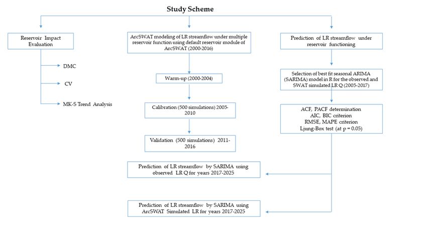
Remote Sens. 2021, 13, 1382                                                                                         2 of 23

                              number of dams and the total storage capacity of reservoirs rapidly increase [4]. Therefore,
                              knowledge of dam construction and its regulating effects on river discharge is crucial for
                              river and delta management and restoration. Highly regulated rivers in China are subject
                              to large-scale ecosystem amendments made by hydrological alterations. Many of the earlier
                              studies related to dam-induced hydrological alterations across river basins in China focused
                              on the impacts of large dams that generally aim to control floods in large basins, such as
                              the Lancang River [9], the Mekong River [10], the Pearl River [11], the Yangtze River [12],
                              and the Yellow River [13,14]. In addition to large dams, the development of small dams
                              has also been highlighted in national energy policies in China [15]. Therefore, small dam
                              construction is intense in China, especially in South China, where hydropower resources
                              are extensive. Thus, to fill in the knowledge void, the present study focused on the impact
                              appraisal of reservoir functioning in the Lhasa River Basin, a Qinghai–Tibetan Plateau basin
                              in South China (for more information, see Section 2.2). Several researchers have established
                              a number of approaches with the objective of reckoning of the hydrologic modifications
                              caused by human activity. However, hydrological modeling can be an effective alternative
                              for hydrological analysis in different scenarios [16]. The SWAT (Soil and Water Assessment
                              Tool) model developed by the authors of [17] has already been in widespread use for
                              water resource management in many different rivers [18–23]. Additionally, there has been
                              a general lack of applications of physically-based hydrological models to the Yarlung
                              Tsangbo River Basin, especially the Lhasa River Basin [24]. The SWAT model was applied
                              to the Lhasa River Basin in a recent study [25], where streamflow and sediment load were
                              predicted for the Lhasa River in future. The SWAT model was applied to the Lhasa River
                              Basin to simulate its streamflow variability under reservoir influence [26]. The SWAT model
                              was utilized in [27] for hydrological drought propagation in the South China Dongjiang
                              River Basin using the “simulated–observed approach”. Their study estimated the effects of
                              human regulations on hydrological drought from the perspective of the development and
                              recovery processes using the SWAT model.
                                    Streamflow forecasting is of great significance to water resource management and
                              planning. Medium-to-long-term forecasting including weekly, monthly, seasonal, and
                              even annual time scales is predominantly beneficial in reservoir operations and irrigation
                              management, as well as the institutional and legal features of water resource management
                              and planning. Due to their reputation, a large number of forecasting models have been
                              developed for streamflow forecasting, including concept-based, process-driven models
                              such as the low flow recession model, rainfall–runoff models, and statistics-based data-
                              driven models such as regression models, time series models, artificial neural network
                              models, fuzzy logic models, and the nearest neighbor model [28]. Of various streamflow
                              forecasting methods, time series analysis has been most widely used in the previous
                              decades because of its forecasting capability, inclusion of richer information, and more
                              systematic way of building models in three modeling stages (identification, estimation, and
                              diagnostic check), as standardized by Box and Jenkins (1976) [29]. The current study made
                              use of "simulated–observed approach" after [27] for predicting the Lhasa River streamflow
                              under reservoir operations in the Lhasa River Basin. SWAT-simulated and observed
                              hydrological time series were used introduced to a stochastic AutoRegressive Integrated
                              Moving Average (ARIMA) model. As a common data-driven method, the ARIMA model
                              has been widely used in time series prediction due to its simplicity and effectiveness [30].
                              Adhikary et al. (2012) [31] used seasonal ARIMA (SARIMA) model to model a groundwater
                              table. They took weekly time series and concluded that SARIMA stochastic models can be
                              applied for ground water level variations. Valipour et al. (2013) [32] modeled the inflow of
                              the Dez dam reservoir with SARIMA and ARMIA stochastic models. His research results
                              showed that the SARIMA model yielded better results than the ARIMA model. Ahlert
                              and Mehta (1981) [33] analyzed the stochastic process of flow data for the Delaware River
                              by the ARIMA model. Yurekli et al. (2005) [34] applied SARIMA stochastic models to
                              model the monthly streamflow data of the Kelkit River. Modarres and Ouarda (2013) [35]
                              demonstrated the heteroscedasticity of streamflow time series with the ARIMA model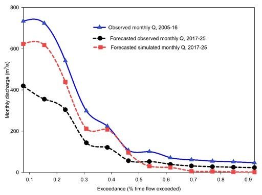
Remote Sens. 2021, 13, 1382                                                                                          3 of 23

                              in comparison to GARCH (Generalized Autoregressive Conditionally Heteroscedastic)
                              models. Their results showed that ARIMA models performed better than GARCH models.
                              Ahmad et al. (2001) [36] used the ARIMA model to analyze water quality data. Kurunç et al.
                              (2005) [37] used the ARIMA and Thomas Fiering stochastic approach to forecast streamflow
                              data of the Yesilurmah River. Tayyab et al. (2016) [38] used an auto regressive model in
                              comparison to neural networks to predict streamflow.
                                   The current study primarily aimed to (i) investigate the reservoir operations’ impact on
                              the Lhasa River discharge, (ii) apply the SWAT model to simulate Lhasa River streamflow
                              under multiple reservoir functioning, and (iii) to predict Lhasa River streamflow under
                              reservoir’s influence using ‘observed’ and ‘SWAT-simulated’ hydrological data series as a
                              step forward in overcoming the data scarcity problem of the area. The study was intended
                              to benefit water resource managers and hydrological engineers in understanding the future
                              hydrological regime in the Lhasa River Basin under reservoir functioning and aiding
                              in developing better management practices and planning for hydrological resources in
                              the area. The current study holds novelty in combining a physical-based hydrological
                              model and a statistical time series forecasting model for the simulation and prediction,
                              of the discharge of the Lhasa River respectively, one of the important rivers in the data-
                              scarce Qinghai–Tibetan Plateau, which is under the influence of recent major hydraulic
                              interventions in the form of the Zhikong and Pangduo hydropower reservoirs.

                              2. Materials and Methods
                              2.1. Study Area—Lhasa River Basin
                                    The Lhasa River Basin (LRB), ranging from 29◦ 190 to 31◦ 150 N and from 90◦ 600 to
                              93◦ 200 E,is the economical and authoritative hub of the autonomous Qinghai–Tibetan
                              plateau (QTP). The Lhasa River (LR) is the longest tributary of the Yarlung Tsangpo River;
                              LRB covers a ≈32,321 km2 basin area (ArcSWAT-estimated area by the digital elevation
                              model used in the current study), comprising 13.5% of the total area of the Yarlung Tsangpo
                              basin [39]. The LRB exhibits typical semi-arid monsoonal climate conditions, where the
                              major proportion of received rainfall is concentrated in the summer season from June to
                              September with the simultaneous generation of peak LR discharge during the same time.
                              Peng et al. (2015) [24] showed that rainfall in summer is a governing feature in producing
                              summer stream flow in the Lhasa River basin. Thus, the rainfall disproportion poses
                              a direct influence on the rainfall-dependent runoff generation phenomena in the basin.
                              The hydrometric and meteorological records for the LRB are maintained at the Pondo,
                              Tanggya, and Lhasa hydrometric stations and the Damxung, Maizhokunggar, and Lhasa
                              meteorological stations, respectively.
                                    The LR stretches to a length of 551 km with a hydropower potential of 1.177 million
                              kWh [39], and it is substantial in fulfilling the hydropower and agricultural requirements
                              of the local community. The LR has been exposed to major hydraulic interventions in the
                              form of reservoir development and confinement during the last and present decades. It
                              is of vital importance to understand the hydrological phenomena of the LRB under the
                              influence of hydraulic structures for a better understanding of the hydrological behavior
                              of the study area to facilitate the understanding of future water resource availability and
                              management in the area. The major hydraulic developments in the study area are the
                              installation of Zhikong and Pangduo hydropower stations over the LR.

                              Zhikong and Pangduo Reservoirs Impoundment on Lhasa River
                                   The Zhikong and Pangduo Dams were built in 2006 and 2013, respectively, on the LR.
                              The Zhikong Dam is located 96 km upstream the urban Lhasa city in the middle and lower
                              reaches of the LR, and it is 65 km downstream the Pangduo Dam, thus impounding the
                              upper LR. To meet the substantially increasing power demand of the Tibet plateau, the
                              Zhikong Dam was built with an installed power capacity of 100 MW and a reservoir water
                              storage capacity of 0.225 billion m3 . The other purposes of this installation include flood
                              control in high rainfall months and irrigation water supply in low rainfall spells during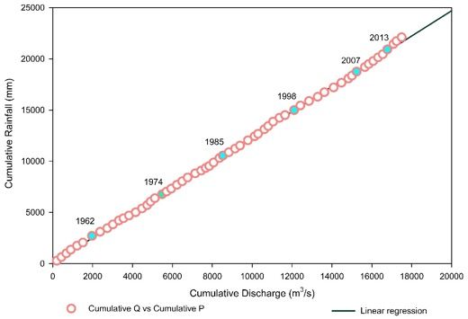
Remote Sens. 2021, 13, x FOR PEER REVIEW 4 of 24
Remote Sens. 2021, 13, 1382 4 of 23
water storage capacity of 0.225 billion m3. The other purposes of this installation include
flood control in high rainfall months and irrigation water supply in low rainfall spells
during the year. However, Wu et al. (2018) [39] showed that impoundment by the Zhikong
the year.
Dam However, Wu
unswervingly et al.the
altered (2018) [39] showed
hydrological that impoundment
behavior by thechannels
of the downstream ZhikongofDam
the
unswervingly altered the hydrological behavior of the downstream channels
LR. The succeeding major hydrological intervention on the LR was the construction of the LR.
of the
The succeeding major hydrological intervention on the LR was the 3construction of the
Pangduo Dam with 160 MW of installed capacity and 1.23 billion m3 of reservoir water
Pangduo Dam with 160 MW of installed capacity and 1.23 billion m of reservoir water
storage capacity. The development purposes of the Pangduo water conservancy project
storage capacity. The development purposes of the Pangduo water conservancy project
include irrigation water availability, power generation, and flood control. It is the pillar
include irrigation water availability, power generation, and flood control. It is the pillar
project and a leading reservoir developed for the enormous growth of the LRB.
project and a leading reservoir developed for the enormous growth of the LRB.
2.2.
2.2. Datasets
Datasets Used
Used
The
The current study
current study utilized
utilized an arrangement of
an arrangement of hydro-meteorological
hydro-meteorological and
and geospatial
geospatial
information
information of the LRB in order to establish the desired results. The datasets included the
of the LRB in order to establish the desired results. The datasets included the
following.
following.
2.2.1.
2.2.1. Geospatial
Geospatial Data
Data of
of LRB
LRB
To extract the
To extract the topographical
topographicalfeatures
featuresofofthe
theLRB,
LRB,a 90
a 90
mm resolution
resolution Advanced
Advanced Ther-
Thermal
mal Emission
Emission and Reflection
and Reflection Radiometer,
Radiometer, GlobalElevation
Global Digital Digital Model
Elevation Model
(ASTER, (ASTER,
GDEM) was
GDEM)
developed wasfordeveloped for the
the study area study
(Figure 1).area
The (Figure
land use1). The land
features useLRB
of the features of the LRB
were established
were
usingestablished using Landsat-8
Landsat-8 Operational Land Operational
Imager (OLI)Land Imager
imagery with(OLI)
a 30 mimagery withThe
resolution. a 30 m
best
cloud free images,
resolution. The bestwith
cloud(137,
free39) and (138,
images, with 39) path
(137, 39) and
and row
(138,respectively,
39) path andwere row used to
respec-
delineate
tively, weretheused
landtouse map forthe
delineate theland
studyusearea
mapusing maximum
for the likelihood
study area classification
using maximum of
likeli-
the land
hood features. The
classification soilland
of the profile of the The
features. LRBsoil
wasprofile
described using
of the LRBFAO-UNESCO
was described (Foodusing
and Agricultural
FAO-UNESCO Organization-United
(Food Nations Educational,Nations
and Agricultural Organization-United Scientific, and Cultural
Educational, Or-
Scien-
ganization)
tific, Harmonized
and Cultural World Soil Database World
Organization)Harmonized versionSoil
1.2 (HWSD
Databasev1.2), a 301.2
version arc-second
(HWSD
rasteradatabase
v1.2), with over
30 arc-second raster15,000 different
database soil mapping
with over units within
15, 000 different the 1:5,000,000
soil mapping scale
units within
FAO-UNESCO Soil Map of the World. All the datasets were projected
the 1:5,000,000 scale FAO-UNESCO Soil Map of the World. All the datasets were projectedto Universal Trans-
verse
to Mercator
Universal 45N projection.
Transverse Mercator All45N
theseprojection.
datasets were mandatory
All these datasetsinput
were formandatory
SWAT model in-
to simulate
put for SWAT themodel
LR streamflow.
to simulate the LR streamflow.
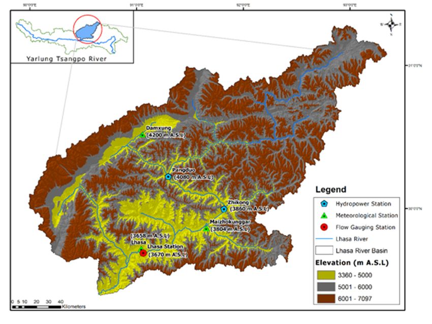
Figure 1. Location map of the Lhasa River Basin extracted from the Advanced Thermal Emission and Reflection Radiometer,
Global Digital Elevation Model (ASTER GDEM) dataset showing hydrological and meteorological stations, hydropower
plants, and some other features of the study area.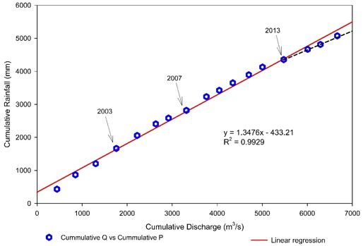
Remote Sens. 2021, 13, 1382                                                                                             5 of 23

                              2.2.2. Hydro-Meteorological Data of LRB
                                   The long-term continuous records for Lhasa River streamflow were obtained from
                              the Lhasa hydrological station located in Lhasa city, 120 km below the Zhikong Dam
                              near the basin outlet. The hydrological data records are maintained at three hydrometric
                              stations, but the current study utilized the data records of the Lhasa station because they
                              represented the total river discharge contributed from the entire catchment from 1956
                              to 2016. For data on the required climatic variables in the current study, the long-term
                              data from three meteorological stations—Damxung, Maizhokunggar, and Lhasa—were
                              used. The meteorological dataset includes records of daily precipitation, maximum and
                              minimum temperature, relative humidity, wind speed, and sunshine hours. Data on these
                              climate variables were fed into the SWAT model to simulate LR streamflow.

                              2.3. Method
                              2.3.1. Reservoir Impact Assessment on LR Discharge
                                   The current study intended to estimate the impact of reservoir functioning by using
                              the modest, graphical, and useful method of double-mass curve (DMC) analysis for the
                              consistent and long-term trend examination of hydro-meteorological data. The concept
                              of the double-mass curve is that a plot of the two cumulative quantities during the same
                              period displays a straight line as long as the proportionality between the two remains
                              unchanged, and the slope of the line represents the proportionality. The advantages of
                              this method are that it can smooth a time series and eliminate random components in the
                              series, thus showing the main trends of the time series. In last 30 years, Chinese researchers
                              have explored the effects of soil and water conservation measures and land use/cover
                              changes on runoff and sediment using the DMC method, resulting in some very good
                              outcomes [40]. For the current study, the double-mass analysis of annual LR discharge and
                              LRB precipitation for the long time span of 1956–2016 and the chosen study time period
                              from 2000 to 2016 were done separately to ensure the accuracy and verification of the
                              change points, if any, in the hydrological time series.
                                   The coefficient of variation (CV) was used to determine the variability of climatic and
                              hydrological changes in the LRB by using the long-term available hydro-meteorological
                              time series. CV is defined as:
                                                                           σ
                                                                    CV = ∗ 100%                                          (1)
                                                                           µ
                              where ‘σ’ is the standard deviation and ‘µ’ is the mean.
                                     The construction and operation of water conservancy projects (dams, channel modifi-
                               cations, drainage works, etc.) have transformed the seasonal distribution of and caused
                               abrupt changes in streamflow at the basin scales [41–43]. How to attribute the physi-
                               cal causes of hydrological variability and how to correctly identify the human-caused
                               signals from natural hydrological variability are therefore important questions [44–46].
                               Understanding hydrological variability is initially needed to solve these queries, as well
                               as for hydrological simulation and forecasting, water resource management, control of
                              water disasters, and many other water activities [47]. However, the correct detection and
                               attribution of complex variability in hydrological processes at multi-time scales are still
                               challenging tasks [48,49], and the difficulty has not been resolved, although many methods
                               are presently used [50,51]. There have been a large number of methods such as the moving
                              T-test (Student’s T-test) [52], moving F-test (also known Fisher-Snedecor distribution) [53],
                               Mann–Kendall test [54], and Pettitt test [55]. The evaluation of a trend in time series of
                               hydro-meteorological phenomena has been done using the non-parametric Mann–Kendall
                               test (MK) [56–58] in the MS Excel software supported by XLSTAT 2014 macro. This test is
                               extensively used and can deal with missing and distant data. The test has two parameters
                               that are substantial for trend detection: a significance level (p) that represents the power of
                               the test and a slope magnitude estimate (MK-S) that represents the direction and volume of
                               the trend. The trends in time series were completed by a calculation of Kendall coefficient
                              ‘τ’ [59–61]. In the current study, the MK trend at a significance level of 5% (p < 0.05) was ap-
Remote Sens. 2021, 13, 1382 6 of 23
plied to the hydro-meteorological time series. Specific attention was paid to the streamflow
exposure of the LR to the impact of reservoir operations by analyzing the MK trend and
changes in it with time.
2.3.2. SWAT Modelling of LR Streamflow
The SWAT model is among the most extensively applied open source, semi-distributed
watershed-scale hydrologic models to simulate the water quantity, surface runoff, and qual-
ity of streamflow in river channels [62]. According to the working principle of the SWAT
model, a watershed is initially divided into sub-basins, and each sub-basin is subdivided
into hydrologic response units (HRUs) based on land use, topography, soil, and slope maps.
The hydrologic cycle for each HRU is simulated based on the water balance, including pre-
cipitation, interception, surface runoff, evapotranspiration, percolation, lateral flow from
the soil profile, and return flow from shallow aquifers. In this study, ArcSWAT2012 running
on an ArcGIS 10.2 platform was used for watershed delineation and sub-basin discretiza-
tion, resulting in 21 sub-basins that were further categorized to 149 HRUs. Srinivasan et al.
(2010) [63] stated that since the accuracy of simulated streamflow may be reduced by not
considering a reservoir or dam in a watershed, the calibration of the reservoir component is
needed to improve the accuracy of simulated streamflow. The SWAT model provides four
different reservoir outflow estimation methods: measured daily flow, measured monthly
flow, average annual release rate for uncontrolled reservoir, and controlled outflow with
target release. The selection of the method depends on available data regarding the reser-
voir. Therefore, the SWAT model was forced to simulate LR streamflow under the reservoir
influence by using the default reservoir module of SWAT. The reservoir details including
surface area, reservoir water volume, reservoir operational year, and monthly LR discharge
data for the time span of 2000–2016 were poured into the model to simulate LR discharge
under the hydraulic interventions of the Zhikong and Pangduo dams. The model was
calibrated for the years 2005–2010 and validated for 2011–2016 with 500 simulations each
using SWAT-CUP (SWAT Calibration and Uncertainty Procedures) algorithm. The global
sensitivity method was used to rank the selected sensitive parameters.
The sensitivity and significance degree of each parameter were analyzed by the t-Stat
and p-value, as well as the p-factor and r-factor; the higher the value of t-Stat, the greater
its sensitivity is, and the lower the p-value, the greater the sensitivity is. The p-factor is
the percentage of data that is enclosed by the 95PPU (95 Percent Prediction Uncertainty)
band (ranging from 0 to 1, where 1 shows that all the prediction are within the 95PPU
band), while the r-factor is the average width of the 95PPU band divided by the standard
deviation of the measured variable (from 0 to ∞, with 0 showing perfect match). During the
calibration and validation periods, the calculated monthly streamflow was compared with
the observed data from the Lhasa hydrometric station using the Nash–Sutcliffe coefficient
(NSE) [64], the coefficient of determination (R2 ) [65], and the percent bias (PBIAS, %) [66].
Additionally, the observed and simulated discharge records were statistically tested for the
correspondence between them using Pearson correlation [67], Spearman’s correlation [67],
and Kendall’s rank correlation [68] for the credibility verification of SWAT modelling under
the reservoir operations for LR streamflow simulation. Additionally, the forecasted river
discharges using the observed and simulated hydrological time series were correlated
using the same correlation tests.Remote Sens. 2021, 13, 1382 7 of 23
2.3.3. ARIMA Forecasting of LR Discharge Time Series
An ARIMA time series model, which was pioneered by Box and Jenkins (1970), was
employed in this study [28]. In the ARIMA (p, d, and q) model, where, p is autoregressive
(AR), d is differencing, and q is moving average (MA). ARIMA models have two common
forms: one is non-seasonal ARIMA (p, d, and q) and the other is seasonal ARIMA (p, d,
and q) (P, D, and Q) S, where P, D, and Q represent seasonal parts and p, d, and q are
non-seasonal parts of the model. SARIMA was applied in the current study using the
observation-based LR discharge recorded at the Lhasa hydrometric station and the SWAT-
simulation-based LR discharge to predict the future hydrological time series for the LRB.
The SARIMA was used for predicting the LR discharge using both the observed and
simulated hydrological time series in R. The SARIMA models can be used for stationary
time series data, which was ensured through decomposition for non-stationarity and log
transformation for de-seasonality of the SWAT-simulated and observed hydrological time
series. The SARIMA model developed for the observation-based and simulation-based LR
hydrological time series was trained for the time span of 2005–2012 and validated for the
years 2013–2016 under the reservoir influence to minimize the ambiguity in the prediction
of LR streamflow, and LR discharge forecasting was carried out from 2017 to 2025.
We constructed the model and depicted the autocorrelation function (ACF) and partial
autocorrelation function (PACF) of model residuals to confirm autoregressive and moving
average parameters. The final automatic ARIMA model selection was carried out in
the R environment. The ACF and PACF of residuals were determined to evaluate the
goodness of fit. The two most commonly used ARIMA model selection criteria, the
Akaike’s information criterion (AIC) and the Bayesian information criterion (BIC), were
examined and compared for ARIMA model selection. The AIC was used for the purpose
of selecting an optimal model fit to given data. The model that had the minimum AIC was
selected as a parsimonious model [69–72]. The BIC was also utilized for the identification
of the best fit model for LR flow prediction. The model with the least BIC was suitable for
time series prediction [73].
AIC, in general case, is:
AIC = 2k = n1n(SSE/n) (2)
where k is the number of parameters in the statistical model, n is the number of observations,
and SSE is square sum of error given by
n
SSE = ∑ ε2i (3)
i =1
BIC, in general, is given by
BIC = k1n(n) + n1n(SSE/n) (4)
R2 , root mean square error (RMSE), and mean absolute percentage error (MAPE) were
selected to assess the ability of SARIMA in forecasting the LR discharge. A Ljung–Box
test [74] at p = 0.05 was also performed to make sure best fit of the SARIMA model for
both time series for LR discharge. Finally, we applied the best fitted models to forecast
the monthly LR discharge using the observation-based and simulation-based hydrological
time series. The schematic representation of study design is shown in Figure 2.RemoteRemote
Sens. 2021,
Sens.13, 1382
2021, 13, x FOR PEER REVIEW 8 of 238 of 24
Figure 2. Schematic representation of reservoir impact evaluation, seasonal AutoRegressive Integrated Moving Average
(SARIMA) and Soil and Water Assessment Tool (SWAT) model setup for the current study. LR: Lhasa River; DMC: double-
mass Figure 2. Schematic
curve; MK-S: representation
non-parametric of reservoir
Mann–Kendall test;impact evaluation,
CV: coefficient seasonal AutoRegressive
of variability; Integrated Moving
PACF: partial autocorrelation Average
function;
AIC: Akaike’s information criterion; BIC: Bayesian information criterion; RMSE: root mean square error; MAPE: mean dou-
(SARIMA) and Soil and Water Assessment Tool (SWAT) model setup for the current study. LR: Lhasa River; DMC:
ble-mass curve; MK-S: non-parametric Mann–Kendall test; CV: coefficient of variability; PACF: partial autocorrelation
absolute percentage error; Q: Discharge (m3 /s).
function; AIC: Akaike’s information criterion; BIC: Bayesian information criterion; RMSE: root mean square error; MAPE:
mean absolute percentage error; Q: Discharge (m3/s).
3. Results
3.1. Reservoir
3. ResultsImpact Evaluation on Lhasa River Flow
3.1.1.3.1.
Double-Mass CurveEvaluation
Reservoir Impact Analysis on
of Lhasa RiverFlow
Lhasa River Flow
To reckon LR discharge change under reservoir influence, DMC analysis, along with
3.1.1. Double-Mass Curve Analysis of Lhasa River Flow
regression lines for two time spans, was carried out to better understand the hydrological
phenomena To reckon
and theLR discharge
likely changechange
years under
in the reservoir
time series.influence, DMC analysis,
The double-mass along
curves for with
regression lines for two time spans, was carried out to better understand
annually recorded rainfall and discharge, following the work of Searcy and Hardison the hydrological
phenomena
(1960) [75], were and the likelyapplied
individually change for
years
theintime
the time
spansseries. The double-mass
of 1956–2016 curves for
and 2000–2016
annually recorded rainfall and discharge, following the work of
(Figures 3 and 4) respectively. The application of individual cumulative mass curves Searcy and Hardison
for
(1960)spans
two time [75], were individually
was done with theapplied
aim offor the time spans
developing a moreof valid
1956–2016 and 2000−2016
and reliable impact (Fig-
ures 3 and
assessment 4) respectively.
in terms of change in The
theapplication
hydrologicalof time
individual cumulative
series of the LR. mass curves for two
time
The DMC analysis of LR discharge from 1956 to 2016 revealed and
spans was done with the aim of developing a more valid reliable
a nearly impact assess-
proportional
ment in terms of change in the hydrological time series of the LR.
behavior of the rainfall in correspondence to the measured LR discharge. However, we
saw certain years of change along the time series that served as break points in the pattern
of high and low flows in the LR discharge. The years for change are highlighted and
indicated in Figure 3, where the pattern of streamflow breaks to differ from the preceding
years. The result of the long-term DMC analysis was the identification of the change years,
of which the years 2007 and 2013 were of particular significance for the current study.
These two years marked the operation of the two major reservoirs (Zhikong and Pangduo,
respectively) that were considered for the current study. The impact of chosen reservoir
functioning on the hydrological behavior of the LR manifested itself in the long-term
DMC analysis.
To further understand the phenomena of reservoir influence on LR discharge, double-
mass analysis was applied to the time series from 2000 to 2016 (Figure 4), and we saw three
identified change points in the time series during these years.Remote Sens. 2021, 13, 1382 9 of 23
21, 13, x FOR PEER REVIEW 9 of 24
021, 13, x FOR PEER REVIEW 10 of 24
FigureFigure 3. Double-mass
3. Double-mass curve
curve for for cumulative
cumulative rainfall
rainfall and and cumulative
cumulative discharge ofdischarge
the Lhasaof the Lhasa
River for the River
time span of
for the
1956–2016. Thetime
yearsspan of 1956−2016.
for change The years
in hydrological timefor change
series in hydrological
are highlighted time series
and supported are highlighted
by text.
and supported by text.
The DMC analysis of LR discharge from 1956 to 2016 revealed a nearly proportional
behavior of the rainfall in correspondence to the measured LR discharge. However, we
saw certain years of change along the time series that served as break points in the pattern
of high and low flows in the LR discharge. The years for change are highlighted and indi-
cated in Figure 3, where the pattern of streamflow breaks to differ from the preceding
years. The result of the long-term DMC analysis was the identification of the change years,
of which the years 2007 and 2013 were of particular significance for the current study.
These two years marked the operation of the two major reservoirs (Zhikong and Pangduo,
respectively) that were considered for the current study. The impact of chosen reservoir
functioning on the hydrological behavior of the LR manifested itself in the long-term DMC
analysis.
To further understand the phenomena of reservoir influence on LR discharge, dou-
ble-mass analysis was applied to the time series from 2000 to 2016 (Figure 4), and we saw
three identified change points in the time series during these years.
Figure
Figure 4. 4. Double-mass
Double-mass curve
curve for the for the cumulative
cumulative rainfall anddischarge
rainfall and cumulative cumulative discharge
of the of the
Lhasa River Lhasa
for the time span of
River for the time span of 2000−2016. The years for change in hydrological
2000–2016. The years for change in hydrological time series are supported by the text. time series are sup-
ported by the text.
The year 2003 showed a change, as the maximum rainfall was recorded in this year
and produced the simultaneously highest discharge during the year for the chosen study
time period. The next identified change year was 2007, which deviated from the streak of
data points along the regression line. This was the time when one of the selected reservoirsRemote Sens. 2021, 13, 1382 10 of 23
The year 2003 showed a change, as the maximum rainfall was recorded in this year
and produced the simultaneously highest discharge during the year for the chosen study
time period. The next identified change year was 2007, which deviated from the streak of
data points along the regression line. This was the time when one of the selected reservoirs
in the study was built on the LR. The Zhikong hydropower station was completed in
2006 and started functioning in September 2007. The most prominent break point in the
hydrologic time series was identified in 2013 when the second major reservoir started
operating on the LR, i.e., the Pangduo hydropower station, where the data points deviated
from the regression line and indicated a peculiar hydrological behavior in the LRB. Yet
again, the hydraulic interventions demonstrated themselves in the form of change points
across the study time span of hydrologic time series.
3.1.2. Variation Assessment of Lhasa River Streamflow under Reservoir Operations
Figure 5 shows the inter-annual variation of the hydro-meteorological behavior of the
LRB along the two time phases. The CV for the hydro-meteorological phenomena from
1956 to 1999 and from 2000 to 2016 exposed an aggravated variability in the latter time
span compared to the previous time span. The CV of 24% for LRB precipitation during
1956–1999 was lowered to 20% in the second time span of 2000–2016; however, the CV
values for both time spans were relatively closer, which means that the change in the
pattern of precipitation advanced with a greater pace in the study time span compared to
the former long time span of 1956–1999. Similarly, for the annual temperature, the CVs of
Remote Sens. 2021, 13, x FOR PEER REVIEW 11 of 24
8% and 6% for the time spans of 1956–1999 and 2000–2016, respectively, were again closer
values and revealed a faster temperature change in the LRB during 2000–2016.
FigureFigure 5. Changes
5. Changes of annual
of annual river
river discharge(at
discharge (atthe
the Lhasa
Lhasa hydrometric
hydrometricstation),
station),annual mean
annual meantemperature, and annual
temperature, and annual
recorded precipitation for the Lhasa River Basin from 1956 to 1999 and from 2000 to 2016 (study time
recorded precipitation for the Lhasa River Basin from 1956 to 1999 and from 2000 to 2016 (study time period period with reservoirs
with reser-
voirs functioning
functioningininthe study
the area).
study area).
Since it is a typical QTP catchment, the LRB is prone to complex climate change
phenomena
Since it is[25]. TheseQTP
a typical climate variables the
catchment, are closely
LRB isassociated with the hydrologic
prone to complex cycle. phe-
climate change
Particularly for the LRB, the LR discharge is furnished by the precipitation
nomena [25]. These climate variables are closely associated with the hydrologic cycle. [25], and Par-
ticularly for the LRB, the LR discharge is furnished by the precipitation [25], and variabil-
ity in rainfall poses a direct influence on the hydrological behavior of the LRB. Tempera-
ture is also an important feature in determining hydrological phenomena because it as-
serts its influence in the form of evapotranspiration, and, thus, variations in the tempera-Remote Sens. 2021, 13, 1382 11 of 23
variability in rainfall poses a direct influence on the hydrological behavior of the LRB.
Temperature is also an important feature in determining hydrological phenomena because
it asserts its influence in the form of evapotranspiration, and, thus, variations in the
temperature of the LRB may have a potential impact on the water resources in the area.
The CV values for LR discharge revealed an increased variability in 2000–2016 com-
pared to 1956–1999. The CV of 25% for 1956–1999 copiously increased to 34% during the
study time span of 2000–2016. With rainfall being the determining factor for discharge in
the LRB, we saw that during the years of 1956–1999, the CV for rainfall and LR discharge
were very close at 24% and 25%, respectively, thus indicating a close correspondence among
them. Conversely, a large difference in the variability of rainfall and LR discharge was
unveiled during the study time span of 2000–2016. This signified that during this time
span, apart from the climatological justification, some other factor proclaimed its influence
on the LR’s hydrological dynamics.
The LR was subjected to some major hydraulic interventions during the years of
2000–2016, and the increased discharge alteration can be well-attributed to the reservoir
operations in the LRB during this time period. The Zhikong and Pangduo reservoirs became
operational in 2006 and 2013, respectively, establishing a clearly visible modification in the
LR’s hydrological regime, as presented in Figure 5. The LRB is experiencing an aggravated
climatological variation accompanied with human interferences, resulting in a substantially
altered hydrological phenomena in the area that warrants better planning and management
practices in future.
3.2. MK-S Trend Analysis on Lhasa Streamflow under Reservoir Influence
Investigations of the trends in the time series of hydrological data were found to be
an imperative means for the detection and understanding of changes in a rainfall–runoff
process. Their results are exploitable in water management planning and flood-protection.
Climatic changes, together with a different type and stage of human impact, are considered
to be the main causes of rainfall–runoff changes [76]. In the current study, an MK-S test was
applied to determine the direction and magnitude of the trend of hydro-meteorological
phenomena of the LRB; the findings are presented as Table 1.
Table 1. Trend analysis on hydro-meteorological variables of the Lhasa River Basin. MK–τ represents Mann–Kendall’s trend
at p = 0.05 (bold values are significant at p-value), and S represents the Sen’s slope estimator for change. The negative sign
indicates a decrease.
Rainfall (P) Temperature (T) Discharge (Q)
1956–1999 2000–2016 1956–1999 2000–2016 1956–1999 2000–2016
MK–τ 0.04 −0.13 0.54 0.44 0.03 −0.41
S 0.52 (mm yr−1 ) −4.30 (mm yr−1 ) 0.03 (◦ C yr−1 ) 0.06 (◦ C yr−1 ) 0.30 (m3 s−1 yr−1 ) −14.02 (m3 s−1 yr−1 )
Dams influence variations in river discharge, particularly over seasonal time scales [77,78].
The seasonal variation in LR discharge is presented in Table 2, where maximum variation is
shown to be have been experienced by the high flow months of the wet monsoonal season
from June to October with a CV value of 62%, followed by the spring season from March
to May with a CV value of 56%. The dry winter season from November to February was
found to experience the minimum variability with a CV of 47%.
3.3. Lhasa River Streamflow Simulation and Prediction
3.3.1. SWAT Modeling of Lhasa River Flow under Reservoir Influence
In the current study, the SWAT model identified nine parameters sensitive to the
runoff generation phenomena of the LRB. The sensitivity, ranges, and optimum values of
the selected parameters for the study (as identified by SUFI-CUP) are presented in Table 3.
The model ranked SOL_BD, EPCO, GW_REVAP, ESCO, and GW_DELAY as the most
influential parameters in controlling the runoff phenomena in the LRB. This indicatedRemote Sens. 2021, 13, 1382 12 of 23
that the LR discharge is predominantly controlled by the soil physical characteristics,
evapotranspiration, and ground water processes in the LRB. This was supported by the
previously discussed seasonal MK-S trend results for LR discharge, which also indicated a
strong association of evapotranspiration phenomena and ground water movement in the
LRB in the runoff generation process, particularly in the dry winter season.
Table 2. The change and trend on seasonal Lhasa River discharge for the time period of 2000–2016.
CV stands for coefficient of variation, MK–τ represents Mann–Kendall’s trend at p = 0.05 (bold values
are significant at p), and S represents the Sen’s slope estimator for change in LR discharge (m3 s−1
month−1 ). The negative sign indicates a decrease.
Dry Winter Season Spring Season Wet summer Season
(Nov-Feb) (Mar-May) (Jun-Oct)
CV 47% 56% 62%
MK–τ −0.28 −0.14 −0.27
S −0.6 (m3 s−1 yr−1 ) −0.4 (m3 s−1 yr−1 ) −5.6 (m3 s−1 yr−1 )
Table 3. Sensitivity of selected parameters in influencing Lhasa River flow.
Method Range
No Parameter Parameter Description Fitted Value t-stat p-Value Rank
chosen Min-Max
1. r__SOL_BD Soil bulk density (mg/m3 ) Relative −0.5–0.5 0.17 2.287 0.045 1
Plant uptake compensation
2. v__EPCO Replace −1–1 0.65 1.830 0.097 2
factor
Ground water “revap”
3. v__GW_REVAP Replace 0.02–0.2 0.13 1.249 0.240 3
coefficient
Soil evaporation
4. v__ESCO Replace 0.01–1 0.85 −0.711 0.492 4
compensation factor
5. v__GW_DELAY Ground water delay (days) Replace 0–500 12.50 0.630 0.542 5
Manning’s “n” value for
6. r__OV_N Relative −0.5–0.5 −0.02 0.397 0.699 6
overland flow
Available water capacity of
7. r__SOL_AWC Relative −0.2–0.2 0.07 −0.204 0.842 7
soil layer (mm H2 O/mm soil)
Saturated hydraulic
8. r__SOL_K Relative −0.5–0.5 0.47 0.182 0.858 8
conductivity (mm/h)
Initial SCS curve number for
9. r__CN2 Relative −0.2–0.0 −0.17 −0.022 0.982 9
soil condition II
“r” denotes the relative method, and “v” denotes the replace method.
The performance of the SWAT model in simulating LR discharge under the chosen
reservoirs’ influence for the time span of 2000–2016 is presented in Figure 6a. A comparison
of observed and simulated LR discharge is shown in Figure 6b. The simulated hydrological
time series corresponded appreciably well to the observed data series and regularly fluctu-
ated with the precipitation pattern. The high peaks were very well captured by the SWAT
model most of the time, particularly during the calibration years (2005–2010), with a few
being under-estimated. For the validation years (2011–2016), the model again managed
to capture the high peaks, but some peaks were under-estimated. The lower flow was
consistently under-estimated by the model. A similar weakness of the SWAT model in
capturing the low flows of the LR was reported in [25]. Overall, the model performed well
in simulating the LR streamflow by conforming to the work of Moriasi et al. (2007) [79],
where the modeling performance was acceptable if R2 > 0.5, NSE > 0.5, and PBIAS < ±25%.
The performance of the SWAT model during calibration and validation is presented in
Table 4. However, the comparison between observed and simulated hydrological data
series revealed an R2 value of 0.75 (Figure 6b), and majority of the values were enclosed byRemote Sens. 2021, 13, 1382 13 of 23
the 95% prediction and confidence interval. Few of the high flow values were dispersed
because they were under-estimated by the model. This confirmed the competency of the
Remote Sens. 2021, 13, x FOR PEER REVIEW
SWAT 14 of 24
model in simulating the LR discharge under the reservoir operations selected for
the current study.
(a)
(b)
FigureFigure
6. (a)6.SWAT
(a) SWAT simulation
simulation of Lhasa
of Lhasa RiverRiver discharge
discharge recorded
recorded at theatLhasa
the Lhasa hydrometric
hydrometric station
station
for time span of 2005–2016. (b) Comparison of observed and SWAT-simulated Lhasa River dis-
for time span of 2005–2016. (b) Comparison of observed and SWAT-simulated Lhasa River discharge
charge from 2005 to 2016.
from 2005 to 2016.
Table 4. Performance of the SWAT model in simulation of Lhasa River flow under reservoir oper-
The association of observed and SWAT-simulated LR discharge was verified by the
ations. p-factor: percentage of data that is enclosed by the 95PPU band; r-factor: the average width
correlation tests presented in Table 5. All the correlation coefficients produced high values
of the 95PPU band divided by the standard deviation of the measured variable (from 0 to ∞, with
and 0thus proved that the SWAT-simulated results could be used to predict the future LR
showing perfect match).
discharge from 2017–2025.
2000–2016 (00–04 warm-up)
No. Performance criteria
Calibration (05–10) Validation (11–16)
1. p-factor 0.96 0.50
2. r-factor 1.09 0.47Remote Sens. 2021, 13, 1382 14 of 23
Table 4. Performance of the SWAT model in simulation of Lhasa River flow under reservoir opera-
tions. p-factor: percentage of data that is enclosed by the 95PPU band; r-factor: the average width of
the 95PPU band divided by the standard deviation of the measured variable (from 0 to ∞, with 0
showing perfect match).
2000–2016 (00–04 Warm-Up)
No. Performance Criteria
Calibration (05–10) Validation (11–16)
1. p-factor 0.96 0.50
2. r-factor 1.09 0.47
3. R2 0.91 0.58
4. NSE 0.86 0.50
5. PBIAS 5.5 5.5
Table 5. Statistical correlation of observed and SWAT-simulated Lhasa River discharge.
No. Correlation Coefficient Value
1. Pearson’s correlation 0.87
2. Spearman’s correlation 0.87
3. Kendall’s rank correlation 0.68
Bold values are significant at p = 0.05.
3.3.2. Seasonal ARIMA Application for Predicting Hydrological Regime of Lhasa River
Basin under Reservoir Operations
While making use of the observed LR hydrological time series to identify the future
trend of LR streamflow under reservoir operations for the years 2017–2025, the SARIMA
model (1, 0, 0) (2, 1, 2)12 was found to be the optimum combination for forecasting of ob-
served streamflow under the cumulative impact of reservoirs by justifying the performance
evaluation criteria presented in Table 6 for attaining the lowest AIC and BIC values, a lower
RMSE value of 0.29 m3 /s, and a MAPE value of only 4.02%—values which confirmed
the validity of the model. The SARIMA model was validated for the years of 2013–2016.
SARIMA produced closely corresponding predicted values for LR streamflow during the
validation time span, with its correlation coefficient of R2 = 0.80 revealing an efficient model
that is capable of predicting the future discharge for the LR. The forecasted monthly LR
discharge was seen to follow a decreasing trend during the time period of 2017–2025 under
reservoir influence (Figure 7a).
Table 6. Performance of SARIMA model in predicting Lhasa River streamflow from 2017 to 2025
using observed and simulated hydrological time series.
Performance Criterion Forecasted Qobs Forecasted Qsim
AIC 76.7 199.4
BIC 91.28 209.12
RMSE 0.29 (m3 /s) 0.65 (m3 /s)
MAPE 4.02% 31.09%
The SARIMA model (1, 0, 0) (2, 1, 0)12 was found to be the optimum combination
for forecasting of SWAT-simulated streamflow under the cumulative impact of reservoirs.
The SARIMA model produced correlation coefficient of R2 = 0.88 for the validation years
from 2013 to 2016 for SWAT-simulated and forecasted LR discharge with a relatively higher
MAPE value of 31.09% (Table 6) for the simulation-based forecasted LR discharge. The
predicted discharge using the SWAT-simulated hydrological time series likewise showed a
decreasing discharge.Remote Sens. 2021, 13, 1382 15 of 23
Remote Sens. 2021, 13, x FOR PEER REVIEW 16 of 24
(a)
(b)
Figure
Figure 7. (a)
7. (a) Forecastedmonthly
Forecasted monthlyLhasa
LhasaRiver
Riverstreamflow
streamflow for
for time
time span
spanof
of2013–2025
2013–2025using
usingthe observed
the hydrological
observed time
hydrological time
series from 2005 to 2016. SARIMA model validation years from 2013 to 2016 are marked. (b) Forecasted monthly Lhasa
series from 2005 to 2016. SARIMA model validation years from 2013 to 2016 are marked. (b) Forecasted monthly Lhasa
River streamflow for time span of 2013–2025 using SWAT-simulated hydrological time series from 2005 to 2016. SARIMA
River streamflow
model validationforyears
timefrom
span2013
of 2013–2025
to 2016 areusing SWAT-simulated hydrological time series from 2005 to 2016. SARIMA
marked.
model validation years from 2013 to 2016 are marked.Remote Sens. 2021, 13, x FOR PEER REVIEW 17 of 24
Remote Sens. 2021, 13, 1382 16 of 23
The comparison of observation-based and simulation-based LR discharge presented
in Figure 8a showed a very close correspondence between both hydrological time series
with an R2 of 0.90. However, the simulation-based forecasted LR discharge was higher for
The comparison of observation-based and simulation-based LR discharge presented in
high flow months in future. In advancing through the years from 2017 to 2025, the differ-
Figure 8a showed a very close correspondence between both hydrological time series with
ence in the high peaks was seen to be increasing among the observation and simulation-
an R2 of 0.90. However, the simulation-based forecasted LR discharge was higher for high
based forecasted LR discharge, as presented in Figure 8b. However, both hydrological
flow months in future. In advancing through the years from 2017 to 2025, the difference
data series were shown to experience a decrease in the future years researched in the
in the high peaks was seen to be increasing among the observation and simulation-based
study.
forecasted LR discharge, as presented in Figure 8b. However, both hydrological data series
were shown to experience a decrease in the future years researched in the study.
(a)
(b)
Figure 8. (a) Comparison between observation-based and SWAT-simulation-based Lhasa River
forecasted flow from 2017 to 2025. (b) Scatter plot of observation-based and simulation-based
forecasted monthly Lhasa River discharge for 2017–2025.Remote Sens. 2021, 13, x FOR PEER REVIEW 18 of 24
Remote Sens. 2021, 13, 1382 17 of 23
Figure 8. (a) Comparison between observation-based and SWAT-simulation-based Lhasa River forecasted flow from 2017
to 2025. (b) Scatter plot of observation-based and simulation-based forecasted monthly Lhasa River discharge for 2017–
2025.
To corroborate the association of both forecasted hydrological time series, statistical
correlational tests used in the study produced values of ≥0.80 and are presented in Table 7.
To corroborate the association of both forecasted hydrological time series, statistical
This testifies to the
correlational tests credibility
used of the
in the study approach
produced usedofin≥0.80
values the current study andinshows
and are presented Table that
7. This testifies to the credibility of the approach used in the current study and showsdischarge
simulation-based future LR discharge can be a replacement to observation-based that
and be utilized for
simulation-based further
future analyses regarding
LR discharge water resource
can be a replacement management, planning,
to observation-based dis-
distribution,
charge and be hydropower generation,
utilized for further analysesirrigation
regardingscheduling,
water resourceandmanagement,
reservoir operational
plan-
procedures
ning, in the LRB.
distribution, This can
hydropower prove to be
generation, an aid in
irrigation overcoming
scheduling, andthe hydrological
reservoir opera-data
scarcity
tional issue because
procedures in thethe
LRB.LRB iscan
This a quintessential
prove to be anbasin
aid inofovercoming
the QTP with barely observed
the hydrological
data scarcity
data [25]. issue because the LRB is a quintessential basin of the QTP with barely ob-
served data [25].
Table 7. Statistical correlation between forecasted observation-based and simulation-based Lhasa
River discharge,
Table 7. Statistical2017–2025.
correlation between forecasted observation-based and simulation-based Lhasa
River discharge, 2017–2025.
No. Correlation Coefficient Value
No. Correlation coefficient Value
1. Pearson’s correlation 0.95
1. Pearson’s correlation 0.95
2.
2. Spearman’sSpearman’s
correlationcorrelation 0.95
0.95
3. 3. Kendall’s
Kendall’s rank rank correlation
correlation 0.80
0.80
Bold values
Bold valuesare
aresignificant
significant p =p 0.05.
atat = 0.05.
AA flow–duration
flow–durationcurvecurveoffers
offersaapractical
practicalapproach
approachfor forstudying
studyingthe theflow
flowcharacteris-
characteristics
of streams and for examining the association of one basin with another.
tics of streams and for examining the association of one basin with another. A flow–dura- A flow–duration
curve
tion is a cumulative
curve frequency
is a cumulative curvecurve
frequency that shows the percent
that shows of time
the percent of during whichwhich
time during specified
discharges were equaled or exceeded in a given period. A rather easier
specified discharges were equaled or exceeded in a given period. A rather easier concep- conception of the
tion of the flow–duration curve is that it is a streamflow data demonstration combiningflow
flow–duration curve is that it is a streamflow data demonstration combining the
characteristics
the of a stream
flow characteristics throughout
of a stream the ranges
throughout of discharge
the ranges of dischargein in
oneonecurve
curve[80].
[80]. The
The flow–duration curves for the observed LR discharge and forecasted observation- and
flow–duration curves for the observed LR discharge and forecasted observation-based
simulation-based
based LR discharge
and simulation-based are presented
LR discharge in Figurein9.Figure 9.
are presented
Figure 9. Flow–duration curves for the monthly observed, forecasted observation-based, and SWAT-
simulation-based Lhasa River discharge.
We saw that the SWAT-simulation-based predicted LR discharge produced a steeper
sloped curve following the similar high and low flow pattern of the observed LR discharge.You can also read