Influence of the Water Source on the Carbon Footprint of Irrigated Agriculture: A Regional Study in South-Eastern Spain - MDPI
←
→
Page content transcription
If your browser does not render page correctly, please read the page content below
agronomy
Article
Influence of the Water Source on the Carbon Footprint of
Irrigated Agriculture: A Regional Study in South-Eastern Spain
Bernardo Martin-Gorriz , Victoriano Martínez-Alvarez                              , José Francisco Maestre-Valero
and Belén Gallego-Elvira *

                                            Agricultural Engineering Center, Technical University of Cartagena, Paseo Alfonso XIII 48, 30203 Cartagena,
                                            Spain; b.martin@upct.es (B.M.-G.); victoriano.martinez@upct.es (V.M.-A.); josef.maestre@upct.es (J.F.M.-V.)
                                            * Correspondence: belen.gallego@upct.es; Tel.: +34-968177731

                                            Abstract: Curbing greenhouse gas (GHG) emissions to combat climate change is a major global
                                            challenge. Although irrigated agriculture consumes considerable energy that generates GHG emis-
                                            sions, the biomass produced also represents an important CO2 sink, which can counterbalance the
                                            emissions. The source of the water supply considerably influences the irrigation energy consumption
                                            and, consequently, the resulting carbon footprint. This study evaluates the potential impact on the
                                            carbon footprint of partially and fully replacing the conventional supply from Tagus–Segura water
                                            transfer (TSWT) with desalinated seawater (DSW) in the irrigation districts of the Segura River basin
                                            (south-eastern Spain). The results provide evidence that the crop GHG emissions depend largely on
                                            the water source and, consequently, its carbon footprint. In this sense, in the hypothetical scenario of
                                            the TSWT being completely replaced with DSW, GHG emissions may increase by up to 50% and the
                                  carbon balance could be reduced by 41%. However, even in this unfavourable situation, irrigated

                                            agriculture in the study area could still act as a CO2 sink with a negative total and specific carbon bal-
Citation: Martin-Gorriz, B.;                ance of −707,276 t CO2 /year and −8.10 t CO2 /ha-year, respectively. This study provides significant
Martínez-Alvarez, V.; Maestre-Valero,
                                            policy implications for understanding the water–energy–food nexus in water-scarce regions.
J.F.; Gallego-Elvira, B. Influence of the
Water Source on the Carbon Footprint
                                            Keywords: agricultural irrigation; climate change; GHG emissions; carbon removal; water transfer;
of Irrigated Agriculture: A Regional
                                            desalination; water–energy nexus
Study in South-Eastern Spain.
Agronomy 2021, 11, 351. https://
doi.org/10.3390/agronomy11020351

Academic Editor: Benjamin D. Duval,
                                            1. Introduction
Sarah C. Davis and Darren Drewry                  Anthropogenic greenhouse gas (GHG) emissions are the key driver of climate change [1].
Received: 29 December 2020                  Population growth, economic prosperity and evolving dietary demands are increasing
Accepted: 13 February 2021                  the demand for food. The way we produce and consume (intensive farming systems,
Published: 16 February 2021                 water and soil depletion, high levels of greenhouse gas emissions, etc.) needs profound
                                            changes to maintain productivity whilst promoting sustainability and resilience of the
Publisher’s Note: MDPI stays neutral        agro-systems [2]. In the context of promoting crop productivity and sustainability, irrigated
with regard to jurisdictional claims in     agriculture may be one of the main suitable options against climate change [3–5]. An
published maps and institutional affil-     increase in irrigation demand, with the corresponding impact on energy consumption
iations.                                    and GHG emissions, will lead to potential conflicts in terms of mitigation and adaptation
                                            policies [6,7].
                                                  Agricultural sustainability must be monitored based on adequate indicators. The Span-
                                            ish Ministry of Agriculture, in its Annual Report of Indicators [8], considers GHG emission as
Copyright: © 2021 by the authors.           an adequate indicator to provide an integrative vision of the agricultural sector sustainabil-
Licensee MDPI, Basel, Switzerland.          ity. From the perspective of climate change and its mitigation, agriculture can contribute to
This article is an open access article      both climate change and its mitigation. In the agricultural sector, GHG emissions come
distributed under the terms and             from the applied production techniques as well as from provided inputs (i.e., fertilisers,
conditions of the Creative Commons          agrochemicals, irrigation water supply, energy supply). However, agriculture represents a
Attribution (CC BY) license (https://
                                            carbon sink, capturing atmospheric CO2 into the plant mass and the soil. Consequently,
creativecommons.org/licenses/by/
                                            an analysis of the carbon footprint in agriculture needs to determine the carbon balance
4.0/).

Agronomy 2021, 11, 351. https://doi.org/10.3390/agronomy11020351                                             https://www.mdpi.com/journal/agronomy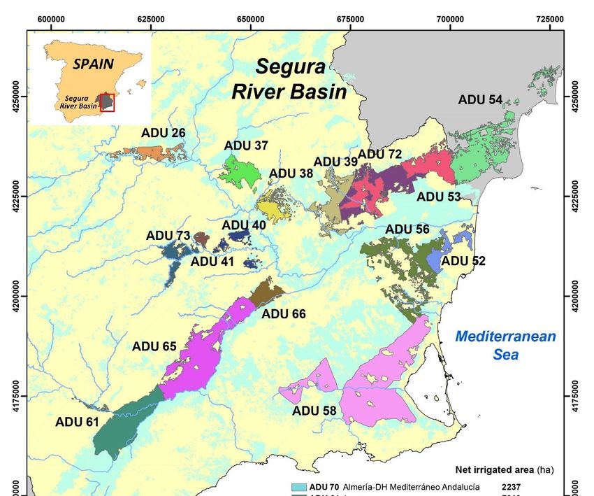
Agronomy 2021, 11, 351                                                                                            2 of 19

                         between GHG emission and CO2 removal. A negative balance implies that the activity
                         captures more CO2 than it emits and therefore can be considered sustainable from a climate
                         perspective. However, a positive balance implies the need to seek mitigation strategies
                         such as innovative production techniques and alternative inputs to achieve sustainability.
                               Life Cycle Assessment (LCA) is a reference method to quantitatively evaluate the
                         environmental impact across the entire supply chain in terms of energy-use efficiency,
                         environmental effects and sustainability, including GHG emissions as a relevant indicator
                         of global warming potential. For agri-food systems, LCA is increasingly being used
                         to evaluate and analyse environmental and food security issues [9,10], including crop
                         production [11,12], contributing to the creation of scientific knowledge for evidence-based
                         policy-making [13].
                               Irrigated agriculture constitutes the largest consumer of freshwater in the water-scarce
                         Mediterranean region and provides a major source of income and employment for rural
                         livelihoods [14]. However, increasing droughts and water scarcity are jeopardising the
                         availability and reliability of water resources for irrigation [15]. This is a limiting factor
                         for economic development and has highlighted concerns regarding the environmental
                         sustainability of agriculture in the region [16]. In this context, inter-basin water transfers
                         are instruments of water planning that can play an important role in mitigating water
                         scarcity and the effects of climate change [17].
                               Our study focuses on irrigated lands associated with the Tagus–Segura water transfer
                         (TSWT); a 292-km-long canal that has transferred flows since 1979 from the Tagus head-
                         waters river basin in central Spain, to the Segura River basin (SRB) in south-eastern (SE)
                         Spain [18,19]. The SRB, despite being hot and dry, has witnessed remarkable agricultural
                         development over the last decades, becoming one of the world’s leading producers of
                         fruits and vegetables [20]. An important part of this highly profitable business relies almost
                         exclusively on the TSWT. Pellicer-Martínez and Martínez Paz [21] studied the possible
                         effects that the latest climate change scenarios may have on the TSWT and predicted impor-
                         tant reductions in snowfalls and snow covers, the recharge of aquifers and, consequently,
                         the available water resources in the headwaters of the Tagus River basin. Moreover, the
                         importance of water ecosystem services in the Tagus River basin has progressively been
                         highlighted in recent years. The latter involves increasing demands to satisfy and safe-
                         guard multiple needs of consumers, the economy and the environment. Consequently, the
                         decrease in water available for the transfer has led to bitter regional disputes [22]. Past and
                         present perspectives on the SRB water shortage are well documented [19,23].
                               This chronic and problematic situation has driven the orientation of Spanish water
                         policy since the beginning of the 21st century towards the widespread adoption of non-
                         conventional water resources. Particular emphasis has been given to desalination as an
                         alternative to other water supply options such as river regulation or new inter-basin water
                         transfers [24]. As a result, massive seawater desalinisation has been implemented in the last
                         decade as an alternative way to increase urban and agricultural supplies in SE Spain [23].
                         Seawater desalination effectively removes the climatological and hydrological constraints
                         associated with continental water resources [25]. In addition, it circumvents the social
                         and inter-regional conflicts associated with river regulation through dam building and
                         long-distance inter-basin water transfers [26]. In such a way, desalination is alleviating
                         the decrease in the water supplied by the TSWT in recent years. The downside is that the
                         specific energy consumption for desalinated seawater (DSW) supply in the SRB (4.32 kWh
                         m−3 [27]) is much higher than that of the TSWT (1.21 kWh m−3 [28]). This increases the
                         GHG emissions of irrigated agriculture and jeopardises the effectiveness of climate change
                         control policies.
                               Given the importance of irrigated agriculture in SE Spain, this study provides robust
                         and objective estimates on GHG emissions under different scenarios, in which the TSWT
                         supply is partially and fully replaced with DSW. Furthermore, in order to highlight the
                         potential role of regional agriculture as a carbon sink, the CO2 removals associated with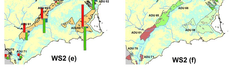
Agronomy 2021, 11, 351                                                                                            3 of 19

                         the irrigation lands were estimated. Finally, potential ways to improve the sustainability of
                         the agricultural use of DSW are proposed.

                         2. Materials and Methods
                               The analysis of the carbon footprint for the study area was developed in two phases:
                         (1) the determination of the GHG emissions and CO2 removals for the most representative
                         crops in the study area; and (2) their extrapolation to the irrigation districts supplied by the
                         TSWT to obtain global figures of the carbon balance.
                               Agricultural production data was used to estimate the carbon footprint for the most
                         representative fruit and vegetable crops in the study area. In order to estimate the GHG
                         emissions, LCA methodology has been applied, following the protocols standardised by the
                         International Standards Organization in the ISO 14040 [29] and ISO 14044 [30] standards.
                         Crop CO2 removal rates were obtained from the results of experimental trials in the region
                         published by other authors, as detailed in Section 2.4.
                               Several studies have found that irrigation water conveyance and application emit
                         large amounts of GHGs [31–33]. Therefore, the carbon footprint was calculated under
                         three water supply scenarios, in which there was a progressive replacement of the water
                         supply from the TSWT with DSW. This is the main strategy included in the Spanish water
                         planning to redress the persistent water deficit affecting irrigation in the SRB. Therefore,
                         the sensitivity of the results for this variable is of special interest to analyse the carbon
                         footprint implications of the planned agricultural water supply. Finally, we compare our
                         results with other related studies.

                         2.1. Segura River Basin (SRB) and Tagus–Segura Water Transfer (TSWT)
                               The SRB is a highly productive agricultural region in SE Spain, whose economy is
                         built primarily on the export of high-value vegetables and fruits. Its semiarid climate
                         is characterised by hot, dry summers and sporadic intense rains in autumn. The mild-
                         temperature winters allow vegetables to be grown in the open field. This area, with
                         high-return agriculture, is usually referred to as ‘the orchard of Europe’ [34], since exports
                         of horticultural products to EU countries may exceed 70% of the total production. It plays
                         a major role in the basin’s economy in terms of production and employment.
                               The SRB is one of the most water-stressed regions in the Mediterranean basin. The
                         official estimation [35] is that the SRB water resources amount to 1602 Mm3 /year, which in-
                         cludes water transferred from central Spain through the inter-basin TSWT (322 Mm3 /year)
                         and DSW (158 Mm3 /year produced in several desalination plants [27]). These resources
                         fail to satisfy a total water demand of 1834 Mm3 /year, which includes 1546 Mm3 /year for
                         irrigated agriculture (84% of the total). The mean annual water deficit amounts to about
                         400 Mm3 [35], threatening the strategic agricultural production and bolstering conflicts
                         between aggravated users [22]. The water shortage and conflicts explain the massive
                         seawater desalination strategy implemented in the SRB by the Spanish government to
                         guarantee the urban supply as well as foster irrigated agriculture [23].
                               The TSWT is one of the largest (292 km) inter-basin infrastructures in southern Europe.
                         The rationale for developing that water transfer was that cities and tourism on the Mediter-
                         ranean coast needed water to grow and that irrigated agriculture in the mild regions of SE
                         Spain could achieve higher water productivity than in the inner regions. The TSWT is man-
                         aged by its own operational rules, which give priority to the water uses in the Tagus River
                         basin and depend on the volume stored in the Tagus headwaters reservoirs. As indicated
                         in the official estimation of the SRB resources [35], currently and on average, barely 60%
                         of the approved flows can be transferred. Such a decrease in the annual transferred flow
                         is a situation that is predicted to intensify in the future as the pressure of climate change
                         mounts in the Tagus River basin [21,36].
                               The increasing water shortage mainly affects irrigated agriculture, which currently
                         amounts to 262,393 ha in the SRB, and has led to a serious problem of overexploitation
                         in many aquifers [37]. The supply to farmers is organised by irrigation districts, which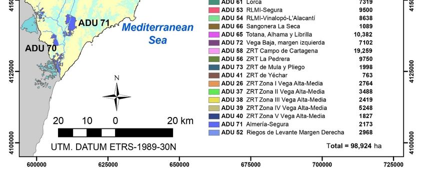
Agronomy 2021, 11, 351                                                                                                   4 of 19

                                 can be differentiated into two types: those using the water resources generated in the SRB,
                                 named ‘traditional irrigation districts’; and, conversely, those that are mainly supplied by
                                 the TSWT, named ‘Tagus–Segura irrigation districts’. Our study targets the latter, which
                                 represents a net irrigated area of 98,923.6 ha organised into 18 Agricultural Demand Units
                                 (ADUs), as shown in Figure 1. They are particularly important in the SRB economy,
Agronomy 2021, 11, x FOR PEER REVIEW                                                                                     5 ofin
                                                                                                                              21
                                 terms of both production value and employment (2000 M EUR/year and 58,500 annual
                                 work units, respectively [35]).

         Figure 1. Study area and Agricultural Demand Units (ADUs) supplied by the Tagus–Segura water transfer (TSWT).
         Figure 1. Study area and Agricultural Demand Units (ADUs) supplied by the Tagus–Segura water transfer (TSWT).

                                2.2. Water Supply Scenarios and Water–Energy Nexus
                                     Irrigation activity is the main water and energy consumer in the production of irri-
                                gated crops under the agroclimatic conditions of the SRB. Agriculture in the SRB is sup-
                                plied with water from different sources: superficial, ground, reclaimed, transferred and
                                desalinated waters. The origin of the irrigation water is a key factor in the specific energy
                                (kWh/m3) associated with the supply [38]. In accordance, the following three water supply
Agronomy 2021, 11, 351 5 of 19
2.2. Water Supply Scenarios and Water–Energy Nexus
Agronomy 2021, 11, x FOR PEER REVIEW 6 of 21
Irrigation activity is the main water and energy consumer in the production of irrigated
crops under the agroclimatic conditions of the SRB. Agriculture in the SRB is supplied with
water from different sources: superficial, ground, reclaimed, transferred and desalinated
waters. 3)
for The origin linked
the ADUs of the irrigation
to the TSWT water is without
[35], a key factor in the specific
considering recentenergy (kWh/m
desalination con-
associated
cessionswith
(13the Mm supply
3/year). [38].
TheInwater
accordance, the availability
resources’ following three water
for this supplyare
scenario scenarios
shown
werein considered:
Figure 2. The specific consumption associated with the supply in WS0 is 0.94
• kWh/m3. scenario (WS0). This is a theoretical scenario corresponding to the irriga-
Concession
• Current
tion rightsscenario
recognised (WS1). This
in the corresponds
Hydrological to the
Plan irrigation
of the rights recognised
Segura Demarcation 2015/21 in the
for
Hydrological Plan of the Segura Demarcation 2015/21
the ADUs linked to the TSWT [35], without considering recent desalination conces-for the ADUs linked to the
TSWT,
sions (13adjusting
Mm3 /year). the TSWT
The water supply to its average
resources’ value
availability forforthisthe period are
scenario 1979 to 2011
shown in
(196 Mm
Figure 3 /year
2. The in origin
specific and 176 Mm³/year
consumption associatedinwith
destination
the supply [39]); and the
in WS0 DSW
is 0.94 to cur-
kWh/m 3.
• rent concessions
Current scenario (13 Mm³/year
(WS1). included in to
This corresponds thethe
Hydrological
irrigation rights Plan recognised
and 80 Mmin/year 3
the
assigned from the Torrevieja desalination
Hydrological Plan of the Segura Demarcation 2015/21 for the ADUsplant, according to the Official
linked Stateto Ga-
the
zette ofadjusting
TSWT, 3 Octoberthe 2019).
TSWT Thissupply
scenario to is
itsquite representative
average value for the of the current
period 1979situation
to 2011
due to
(196 Mm 3 /year
the aforementioned
in origin and 176 Mm3 /year
progressive decrease in the transferred
in destination [39]); andflow through
the DSW the
to cur-
TSWT.
rent The specific
concessions 3
(13consumption
Mm /year included associated with
in the the supply in
Hydrological PlanWS1andis 80
1.41Mm 3 /year
kWh/m 3.
• Substitution
assigned from scenario of TSWT
the Torrevieja with seawater
desalination plant,desalination
according to (WS2). As shown
the Official StateinGazette
Figure
2, this
of is the 2019).
3 October same scenario
This scenario as theis Concession Scenarioof
quite representative (WS0) but replacing
the current situation100% due to of
TSWT with DSW. It represents a hypothetical future scenario that could occur
the aforementioned progressive decrease in the transferred flow through the TSWT.
The specific consumption associated 3.
because of the multiple pressures on with the supply
the TSWT. in WS1consumption
The specific is 1.41 kWh/m associated
• Substitution
with WS3 is scenario
2.78 kWh/m of TSWT
3 . with seawater desalination (WS2). As shown in Figure 2,
this is the same scenario
The specific consumption values as the Concession Scenariowere
for each scenario (WS0) but replacing
calculated based100%on the ofper-
the
TSWT with DSW. It represents a hypothetical future scenario
centage of water provided by each source for this scenario (Figure 2) and their associated that could occur because
of the
specific multiple pressures
consumption on the TSWT.
(the calculation The specific
is included in Tableconsumption associated withMate-
S1 of the Supplementary WS3
is 2.78 kWh/m 3.
rials).
Figure 2. Mix of water sources (Mm3 /year) and the specific energy (kWh/m3 ) by supply scenario. WS0: Concession
scenario; WS1: Current scenario; WS2: Substitution scenario of TSWT with desalinated seawater (DSW).
Figure 2. Mix of water sources (Mm3/year) and the specific energy (kWh/m3) by supply scenario. WS0: Concession sce-
nario; WS1: Current scenario; WS2:
TheSubstitution scenario of values
specific consumption TSWT with desalinated
for each scenarioseawater (DSW). based on the percentage
were calculated
of water provided by each source for this scenario (Figure 2) and their associated specific
2.3. Main Crops
consumption Considered
(the calculationin is
theincluded
Study in Table S1 of the Supplementary Materials).
Estimating GHG emissions for a crop requires all the information regarding the farm-
2.3. work
ing Main Crops Consideredinputs,
and provided in the Study
as well as the necessary infrastructure of the plot. The
estimation of COGHG
Estimating 2 removal usuallyfor
emissions requires
a cropsamples
requiresto all
be taken from complete
the information plant indi-
regarding the
viduals
farminginwork
orderandto determine the carbon
provided inputs, content
as well of all
as the their organs.
necessary Therefore,ofhaving
infrastructure all
the plot.
this information
The estimation offorCOall
2 the crop
removal species
usually developed
requires in the
samples ADUs
to be linked
taken to
from the TSWT
complete is not
plant
aindividuals in order
straightforward to determine
process the carbon
and is often only content
accessibleof all
fortheir organs.
the most Therefore,
relevant having
crops. Nine
crops were selected as being the most representative since they cover the largest area in
the case studied.
The selected crops were organised into three groups (outdoor vegetables, citrus and
non-citrus fruit) in order to comply with the classification of crops in the Hydrological
Plan of the Demarcation of Segura 2015/21 for the description of the ADUs:Agronomy 2021, 11, 351 6 of 19
all this information for all the crop species developed in the ADUs linked to the TSWT is
not a straightforward process and is often only accessible for the most relevant crops. Nine
crops were selected as being the most representative since they cover the largest area in the
case studied.
The selected crops were organised into three groups (outdoor vegetables, citrus and
non-citrus fruit) in order to comply with the classification of crops in the Hydrological Plan
of the Demarcation of Segura 2015/21 for the description of the ADUs:
• Outdoor vegetables. This group is made up of artichoke, broccoli, lettuce and melon.
Their covered area in the region represents 84.42% of the total cultivated vegetables
area [40] (see Table S2 in the Supplementary Materials).
• Citrus. Lemon, mandarin and orange were considered. Their covered area in the
region represents 97.78% of the total cultivated citrus area [40] (see Table S3 in the
supplement for details).
• Non-citrus fruits (fleshy fruits). Apricot and peach were considered. Their covered
area in the region represents 88.02% of the total cultivated non-citrus area [40] (see
Table S4 in the supplement for details).
Table 1 shows the net area by crop group in the set of ADUs associated with the TSWT.
The share was 27.81% for outdoor vegetables, 45.83% for citrus and 12.30% for non-citrus
fruits, covering a total of 85.94% of the irrigated area in the case studied.
Table 1. Net area by crop group in the set of ADUs associated with the TSWT [34].
Crop Surface Area (ha) Percentage (%)
Citrus 45,339.5 45.83
Vegetables, outdoor 27,509.9 27.81
Non-citrus (fleshy fruit) 12,165.3 12.30
Olive 3638.3 3.7
Almond 2975.8 3.0
Cereals, winter 2161.8 2.2
Vegetables, protected 2198.1 2.2
Grapes, table 1704.5 1.7
Grapes, wine 864.8 0.9
Tuber (potato) 241.2 0.2
Cereals, spring (maize) 51.1 0.1
Lucerne 44.1 0.1
Cotton 29.3 0.1
Total 98,923.6 100.00
2.4. Carbon Footprint (CO2 Balance)
The carbon footprint was determined as the difference between the GHG emissions
related with farm operations and CO2 (biogenic carbon) removal by crops. Throughout
the study, the following sign criterion was considered: positive for carbon transfers from
agricultural activity to the atmosphere and negative when transfers occur in the opposite
direction. Therefore, GHG emissions have a positive sign, the removal of CO2 has a
negative sign and the balance sign is the result of the sum of those flows.
In order to determine GHG emissions related with farming operations, the LCA
methodology was applied, following the protocols standardised by the ISO 14040/14044
standard series [29,30]. GHG emissions were estimated following the IPCC 2013 v 1.03
(time frame of 100 years) methodology from the Intergovernmental Panel on Climate
Change [41] and expressed as CO2 eq using the most recent IPPC emission factors [42].
The biogenic carbon dioxide fixation was estimated following ISO 14067 [43] and
reported in terms of CO2 . According to ISO 14067, when calculating the carbon footprint
for a product’s entire life cycle all the emissions and removals (biogenic and fossil) must
be considered, regardless of the crop cycle length. Details of biogenic carbon dioxide
fixation by crops were obtained from Carvajal et al. [44], who presented information forAgronomy 2021, 11, 351 7 of 19
most crops in SE Spain. The carbon sequestration in the soil could not be quantified and
hence considered due to current lack of data, like the actual influence of tillage, organic
amendments and crop rotation on the carbon storage.
2.4.1. Calculation of GHG Emissions by Life Cycle Assessment (LCA) Methodology
In order to determine GHG emissions related with farming operations, the LCA results
obtained in a manuscript recently published by the authors [33] were considered. LCA
was used to quantify the environmentally relevant flows of the most important fruit and
vegetable production systems in SE Spain from several perspectives: depletion of elements
and fossil fuels, acidification and eutrophication hazards, global warming potential and
use of water resources. An LCA sensitivity analysis was used in this study to estimate the
variation in the GHG emissions, considering the specific energy from the supply scenarios
defined above (Section 2.2).
The functional unit was the cultivation of one hectare, throughout one year. The
crop cycle length was one year for citrus (lemon, orange and mandarin) and non-citrus
(apricot and peach) woody crops, and artichoke; six months for broccoli; and four months
for lettuce and melon. In order to compare results between crops throughout one year,
the following five annual crop rotations of outdoor vegetables were considered, because
they are the most frequent and representative in the study area (information provided
by the “Campo de Cartagena” Irrigation District, www.crcc.es): (1) lettuce–lettuce; (2)
lettuce–broccoli; (3) lettuce–melon; (4) broccoli–melon; (5) artichoke. We considered the
average value obtained from those crop rotations as being the annual value per hectare for
outdoor vegetables.
More detailed information regarding the LCA carried out can be found in the
Supplementary Materials, including (i) the system boundaries for the cradle-to-gate pro-
duction of vegetable and woody crops (Figure S1), (ii) the description of the agricultural
stages (Table S5) and (iii) the LCA inventory for the studied crops (Tables S6 and S7). In
addition, the surface area by crop group in each ADU (Table S8) and the annual values of
the carbon balance in each ADU (Tables S9 and S10) are provided.
2.4.2. Calculation of CO2 Removal by Crops
The biogenic carbon dioxide fixation by crops was obtained from the study by
Carvajal et al. [44], which analysed the potential for CO2 removal for the main agricultural
and forestry species in the region. Table 2 shows the carbon removal values (t CO2 /ha) of
the crops under study.
Table 2. Annual values of CO2 fixation (kg CO2 ) per plant and per hectare and planting density (plant/ha) of the main
vegetables and woody crops cultivated in the region [43].
CO2 Fixation Planting Density CO2 Fixation
Crop Group Crop
(kg CO2 /Plant) (Plant/ha) (t CO2 /ha)
Outdoor vegetables Artichoke −1.854 7000 −12.98
Broccoli −0.239 35,000 −8.37
Lettuce −0.130 65,000 −8.45
Melon −0.802 10,000 −8.02
Citrus Lemon −106.93 280 −29.94
Mandarin −31.11 420 −13.06
Orange −49.35 420 −20.73
Non-citrus (fleshy fruit) Apricot −84.49 204 −17.24
Peach −49.77 570 −28.37Agronomy 2021, 11, 351 8 of 19
2.5. Extrapolation of Results to ADUs Supplied by the TSWT
A Geographic Information System (ESRI ArcGIS) was used to extrapolate the values
previously obtained to the entire target area. The steps followed in the extrapolation
process can be summarised as follows:
1. Determination of the annual values of GHG emissions, CO2 removal and carbon
balance for each crop group and water scenario. For the “citrus” and “non-citrus”
fruit groups the value was calculated using the weighted average by the area of each
crop of the selected group in the region (see Tables S3 and S4 for details). In the case
of the “outdoor vegetables” group, the average value obtained from the five most
frequent and representative crop rotations in the study area was considered as an
annual value per hectare (Section 2.4.1).
2. Determination of the weight of each crop group in each ADU. The percentages that
each group of crops represents in each ADU were considered (data included in
Table S8 of the Supplementary Materials). Then, the net area corresponding to the
crop groups was calculated, increasing it in proportion to its magnitude until the total
net area of each ADU was reached.
3. Determination of the total (t CO2 eq /year) and specific (t CO2 eq /ha-year) annual
GHG emissions per ADU and water scenario. From the GHG emissions values
calculated for each crop group, the value corresponding to each ADU was obtained by
multiplying that value by the weight of the crop group in the ADU (t CO2 eq /ha-year)
and by the net area of the ADU (t CO2 eq /year). This process was repeated for each
water scenario.
4. Determination of the total (t CO2 /year) and specific (t CO2 /ha-year) annual CO2
removal and carbon balance per ADU. The same procedure described in step 3
was followed.
5. Aggregation and graphic representation of the entire study area results for each water
scenario. The estimation of the total and specific annual values of GHG emissions,
CO2 removal and carbon balance were carried out by adding the values obtained for
each ADU and water scenario. Finally, those values were graphically presented to
show their spatial trends.
3. Results and Discussion
3.1. Carbon Balance of the Selected Crops
The GHG emissions, CO2 removal and carbon balance for the selected crops and
scenarios are presented in Figure 3. Overall and regardless of the scenario, the vegetables
show greater variability of GHG emissions than the woody crops. The cultivation of
vegetables annually emitted 7.96 ± 2.73, 9.18 ± 3.31 and 12.77 ± 5.03 t CO2 eq /ha for
scenarios WS0, WS1 and WS2, respectively, whereas the figures for the woody crops
were 8.37 ± 0.98, 9.37 ± 1.03 and 12.30 ± 1.21 t CO2 eq /ha. For both the vegetables and
the woody crops, the greatest GHG sources came from irrigation, field operations and
fertilisers. In the case of vegetables, those stages amounted to 88.3, 89.9 and 92.0% of
the total emissions in WS0, WS1 and WS2, respectively. The annual values for woody
crops were somewhat similar: 91.7, 92.6 and 94.4%, respectively. Our results about the
important contribution of irrigation practices in GHG emissions were in agreement with
those reported by other authors for the Mediterranean region. Persiani et al. [45] found
that the highest energy-consuming inputs for a cauliflower–lettuce rotation in southern
Italy were irrigation followed by fertilisers; and the highest GHG emissions were for
water and fertilisers. In this respect, Martin-Gorriz et al. [33] proposed and evaluated
mitigation strategies to reduce GHG emissions for crops in SE Spain. The most promising
impact-mitigation action was the replacement of mineral fertiliser with manure, which
offered potential GHG emissions reductions of up to 10 and 21% for vegetable and woody
crops, respectively.Agronomy 2021, 11, x FOR PEER REVIEW 10 of 21
Agronomy 2021, 11, 351 9 of 19
Artichoke Broccoli Lettuce Melon Lemon Mandarin Orange Apricot Peach
25
20
a)
15
10
t CO2 eq/ha or tCO2/ha
5
0
-5
- 10
- 15
- 20
- 25
- 30
- 35
25
20
b)
15
10
t CO2 eq/ha or tCO2/ha
5
0
-5
- 10
- 15
- 20
- 25
- 30
- 35
25
20
c)
15
t CO2 eq/ha or tCO2/ha
10
5
0
-5
- 10
- 15
- 20
- 25
- 30
- 35
Fertilisers Pesticides Machinery Nursery Irrigation Field operations CO2 Removal Carbon balance
Figure 3. Greenhouse gas (GHG) emissions by crop (expressed as the contribution by stages: fertilisers, pesticides,
Figure 3. Greenhouse gas (GHG) emissions by crop (expressed as the contribution by stages: fertilisers, pesticides, ma-
machinery, nursery, irrigation and field operations), CO2 removal and carbon balance for the three scenarios; (a) WS0, (b)
chinery, nursery, irrigation and field operations), CO2 removal and carbon balance for the three scenarios; (a) WS0, (b)
WS1
WS1and
and(c)
(c)WS2.
WS2.
With regard to CO2 removal, the annual values for the three scenarios were −9.46 ± 2.36
With regard to CO2 removal, the annual values for the three scenarios were −9.46 ±
and −21.87 ± 7.21 t CO2 /ha for the vegetables and the woody crops, indicating that the
2.36 and −21.87 ± 7.21 t CO2/ha for the vegetables and the woody crops, indicating that the
outdoor vegetables fixed a notably smaller amount than the woody crops. This can be
outdoor vegetables fixed a notably smaller amount than the woody crops. This can be
explained by the higher leaf area index and the longer use of the land in woody crops,
explained by the higher leaf area index and the longer use of the land in woody crops,
which stay and fix carbon throughout the whole year. Artichoke was the exception, with
which stay and fix carbon throughout the whole year. Artichoke was the exception, with
its CO2 removal value being 50% higher than that for the rest of the vegetables, as shown
its CO2 removal value being 50% higher than that for the rest of the vegetables, as shown
in Figure 3.
in Figure 3.
In the Concession Scenario (WS0, Figure 3a), the annual emissions from the vegetables
In the Concession Scenario (WS0, Figure 3a), the annual emissions from the vegeta-
ranged from 6.05 t CO2 eq /ha (melon) to 12.01 t CO2 eq /ha (artichoke). Irrigation accounted
bles ranged from 6.05 t CO2 eq/ha (melon) to 12.01 t CO2 eq/ha (artichoke). Irrigation ac-
for 36.7%, which can be attributed to the fossil fuel combustion to produce electricity to
transport water; fertilisers accounted for 23.3%, which is attributed to the electricity usedAgronomy 2021, 11, 351 10 of 19
for its production; whilst field operations accounted for 28.3%, associated to the diesel
consumption by machinery. In the case of the woody crops, the emissions ranged from
7.12 t CO2 eq /ha (apricot) to 9.60 t CO2 eq /ha (mandarin). In this case, irrigation, fertilisers
and field operations represented 35.2, 27.7 and 28.9%, respectively. In this scenario, all
the crops acted as a CO2 sink. On average, the balance for the woody crops was about
nine times more favourable than for the vegetables (−13.49 ± 7.48 vs. −1.49 ± 0.46 t
CO2 /ha). The lemon crop presented the most negative balance and artichoke had the least
negative balance.
The current scenario (WS1, Figure 3b) showed a rise in specific energy consumption
from 0.94 kWh/m3 in WS0 to 1.41 kWh/m3 , which implies an increase in the emissions for
all the crops. For the vegetables, such increases ranged from 12% (lettuce and melon) to
17% (artichoke and broccoli). In WS1, irrigation, fertilisers and field operations accounted
for 45.0, 20.2, 24.6% GHG emissions, respectively. In the case of the woody crops, such
increases ranged from 12% (citrus) to 14% (fleshy fruits). In this case, irrigation accounted
for 42.1%, fertilisers for 24.7% and field operations for 25.8% of the total GHG emissions.
All the crops continued to act as a CO2 sink, except for artichoke and broccoli. Artichoke
became a source of carbon (1.09 t CO2 /ha, i.e., its farming practices emitted more CO2
into the atmosphere than that captured by the crop), whereas broccoli presented an almost
neutral balance (−0.06 t CO2 /ha). On average, the balance was about 45 times more
favourable for the woody crops than for the vegetables (−12.50 ± 7.52 vs. −0.27 ± 1.03 t
CO2 /ha). Lemon was again the crop with the most negative balance.
Regarding the hypothetical substitution of TSWT with DSW (WS2, Figure 3c), the
specific energy reached 2.78 kWh/m3 and the GHG emissions were again higher. For the
vegetables, lettuce and melon GHG emissions increased by 50% (lettuce–melon rotation) to
68% (artichoke–broccoli rotation) compared to WS0. Of the total GHG emissions, irrigation
accounted for 60.5% of GHG emissions, which is attributed to the fossil fuel combustion
for electricity to produce and transport water; fertilisers accounted for 14.5% and field
operations for 17.0%. In the case of the woody crops, emissions increased range from 45%
(citrus) to 53% (fleshy fruits). In this case, irrigation accounted for 55.8%, fertilisers for
18.8% and field operations for 19.7% of the total. In WS2, only the woody crops continued
to be net carbon fixers (−9.57 ± 7.62 t CO2 /ha), whereas all the vegetables acted as a
CO2 source (3.31 ± 2.75 t CO2 /ha), with artichoke being the crop with the highest carbon
balance (7.14 t CO2 /ha) and melon the one with the lowest (1.05 t CO2 /ha).
The annual values of GHG emissions, CO2 removal and carbon balance per crop
group and scenario are summarised in Table 3. The carbon balance became less favourable
for the environment as the specific energy (kWh/m3 ) of the water supply intensified due
to the progressive incorporation of DSW (WS0 → WS1 → WS2). The per-hectare analysis
showed that the GHG emissions for the outdoor vegetables were 60% higher than for the
woody crops in WS0. This is mainly attributed to the higher implementation of inputs in
the vegetables [33]. Such a percentage increased up to 70% in WS2 due to the higher use of
DSW for irrigation. Thus, CO2 removal by the vegetables was always lower than that of the
woody crops. As a result of both behaviours, the annual carbon balance of the vegetables
was 6 (WS0) to 17 (WS2) times lower than for the woody crops. This circumstance means
that outdoor vegetables went from being a carbon sink in WS0 to being a carbon source in
WS2. Therefore, the woody crops were demonstrated to be more effective in mitigating
climate change than the vegetables, but on the other hand, they are riskier crops for farmers
since they are more sensitive to suffering drought in the long term [46].Agronomy 2021, 11, 351 11 of 19
Table 3. Annual values of GHG emissions, CO2 removal and CO2 balance per crop group and scenario.
GHG Emissions CO2 Removal CO2 Balance
Water Scenario Crop Group
(t CO2 eq /ha-Year) (t CO2 /ha-Year) (t CO2 /ha-Year)
W0 Outdoor vegetables * 13.02 −15.91 −2.89
Citrus 8.91 −25.56 −16.65
Non-citrus fruit 7.47 −24.08 −16.60
W1 Outdoor vegetables * 14.90 −15.91 −1.01
Citrus 9.91 −25.56 −15.65
Non-citrus fruit 8.46 −24.08 −15.62
W2 Outdoor vegetables * 20.43 −15.91 4.52
Citrus 12.87 −25.56 −12.69
Non-citrus fruit 10.96 −24.08 −12.72
* Average values for the most frequent annual crop rotations: (1) lettuce–lettuce; (2) lettuce–broccoli; (3) lettuce–melon; (4) broccoli–melon;
(5) artichoke. Note that the values for each crop are provided in Figure 3.
3.2. Carbon Balance by Agricultural Demand Units (ADUs)
Once the annual values of carbon balance per crop group (Table 3), as well as the
weight of each group in the ADUs were estimated (Table S8), the total (t CO2 /year) and the
specific (t CO2 /ha-year) annual carbon balances were calculated within each ADU for the
selected scenarios (Figure 4). The results are given in Tables S6 and S7 for total and specific
annual values, respectively.
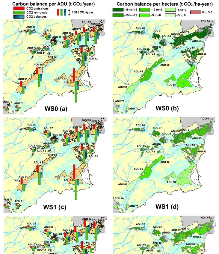
Figure 4a,c,e represent the total GHG emissions, CO2 removals and carbon balance
for the WS0, WS1 and WS2 scenarios, respectively. For WS0 and WS1, all ADUs had a
negative carbon balance, which demonstrates the CO2 sink role of irrigated agriculture
in the study area under concessional and current water supply conditions. The absolute
magnitude of the carbon balances in Figure 4a,c,e were mainly driven by ADU size, though
crop composition played a role (as shown more clearly in 4b, 4d and 4f). The relative
magnitude of an individual ADU among the three scenarios showed the increasing rate
of GHG emissions with the progressive incorporation of DSW. Consequently, the total
carbon balance in each ADU lessened when passing from WS0 to WS1 and lessened still
further for WS2, where ADUs 61, 70 and 71 presented a positive total carbon balance, i.e.,
they became sources of carbon. Therefore, the substitution of TSWT supply with DSW can
change the role of irrigated agriculture from being a carbon sink to being a carbon source
under certain conditions, which are analysed below.
Figure 4b,d,f represent the specific (per hectare) carbon balance for WS0, WS1 and
WS2 scenarios, respectively. A spatial trend of the specific carbon balance value could
be appreciated for all scenarios. It clearly decreased from north to south, but also varied
more subtly from inland to the coast. This variation is related to the crop groups prevailing
in the ADUs (Table S8). Since the southern and coastal zones in the study area present
milder winter conditions and warmer springs, they are far more suitable for winter outdoor
vegetables (broccoli and lettuce) and for early muskmelon crops during the spring–summer
season, for which it is desirable to advance the cultivation date looking for better market
prices. Therefore, the ADUs located in the southern and coastal areas were those with a
higher proportion of outdoor vegetables (ADUs 58, 61, 70 and 71 had from 58 to 79% of
total surface area) and, consequently, those with a less favourable specific carbon balance.
On the contrary, the woody crops were those with a more favourable specific carbon
balance (Table 3) and they predominate in inland and northern ADUs. Non-citrus trees
(fleshy fruits) were those that better tolerated winter cold, which is essential for the proper
development of their annual fruiting cycle, so they are mainly located in more inland
ADUs (ADUs 26, 37, 38, 40, 41 and 73 had from 54 to 86% of total surface area), justifying
their higher specific carbon balance values. Finally, citrus predominate in the northern
area (ADUs 39, 52, 53, 54, 65 and 72 had from 53 to 83% of total surface area), where mild
conditions throughout the year (coastal effect leading to the absence of frost in winter and
very high temperatures in summer) favour their productive cycle. Therefore, the spatialAgronomy 2021, 11, 351 12 of 19
trend of the specific carbon balance value was related to the prevailing location of crops,
explaining the positive total and specific carbon balances of southern ADUs in WS2. The
latter became a carbon source due to the predominance of the only crop group presenting a
positive CO2 balance: outdoor vegetables. It should also be highlighted that citrus, having
shown one of the most negative carbon balances in all scenarios and hence being one of the
most environmentally sustainable crops, is also one of the crops with a lower economic
net margin per cubic metre, as reported in Martínez-Alvarez et al. [23], thus pinpointing
thatREVIEW
Agronomy 2021, 11, x FOR PEER citrus is the crop whose economy would be most affected by the implementation
14 of 21 of an
agricultural supply where DSW was the predominant water source.
Figure 4. Total carbon balance per ADU (t CO /year; a,c,e) and specific carbon balance (t CO2 /ha-year;
Figure 4. Total carbon balance per ADU (t2CO2/year; a,c,e) and specific carbon balance (t CO2/ha-year;
b,d,f) within each
b,d,f) within each
ADU for theADU
considered scenarios:
for the considered WS0 (a,b),
scenarios: WS1
WS0 (a,b), (c,d)
WS1 (c,d)and
and WS2 (e,f).
WS2 (e,f).Agronomy 2021, 11, 351 13 of 19
3.3. Carbon Balance of the Irrigation Lands Supplied by the TSWT
Table 4 shows the total and specific GHG emissions, CO2 removal and carbon balance
for the net irrigated area associated with the TSWT (98,923.6 ha), obtained by adding the
values for each ADU and scenario.
Table 4. Total and specific annual GHG emissions, CO2 removal and carbon balance for the net
irrigated area associated with the TSWT for the considered scenarios.
Scenario GHG Emissions CO2 Removal CO2 Balance
WS0
Total (t CO2 eq /year) 991,744 −2,177,828 −1,208,084
Specific (t CO2 eq /ha-year) 9.61 −22.57 −12.96
WS1
Total (t CO2 eq /year) 1,118,748 −2,177,828 −1,081,080
Specific (t CO2 eq /ha-year) 10.84 −22.57 −11.73
WS2
Total (t CO2 eq /year) 1,492,552 −2,177,828 −707,276
Specific (t CO2 eq /ha-year) 14.47 −22.57 −8.10
Overall, the results show that the irrigated area associated with the TSWT acted as an
important carbon sink regardless of the scenario. This decreasing capacity as a carbon sink
was inversely proportional to the increase in specific energy due to the growing percentage
of DSW in the irrigation mix (from 0.94 kWh/m3 in WS0 to 2.78 kWh/m3 in WS2). In
fact, irrigation was responsible for 36% of the CO2 eq emissions in WS0, with that figure
increasing to 45.0 and 60.5% in the WS1 and WS2 scenarios, respectively.
These figures indicate that, although the incorporation of massive DSW supply to
irrigated agriculture can enhance its resilience in the face of water shortages, such a
strategy does reduce its mitigating role against the increasing CO2 concentration in the
atmosphere. Improved sustainability of irrigated agriculture is needed to compensate for
this undesirable effect. This aspect is discussed below.
4. Adaptation Strategies to Increase Sustainability
At the EU level, agriculture has been responsible for 10% of the GHG emissions in the
last decade [47]. That figure reaches 12% in the case of Spain [48]. Irrigation is currently
responsible for 45.0% of the GHG emissions in the irrigation districts linked to the TSWT
(WS1 scenario), although this could increase to 60.5% in the near future (WS2). Some of
the following strategies can be considered for dealing with that potential increase to foster
sustainability of the DSW agricultural use:
1. Controlled blending of DSW with other water sources. This has been documented in
several countries, including Israel [49–52]; Spain [27,53–55]; Mexico [56,57]; USA (Cal-
ifornia) [58–60]; and Australia [61]. In Israel for example, blending 36% of DSW with
other water sources (groundwater, surface water and brackish water) reduced GHG
emissions by 53% compared to 100% DSW [52]. In the case of La Marina seawater
desalination plant in Almería (south of Spain), mixing the DSW with groundwater did
help remineralise DSW whilst significantly reducing the associated environmental im-
pact [27]. In SE Spain, Martínez-Alvarez et al. [62] evaluated the impact of irrigation
with DSW on farming costs and fertiliser requirements for different crops, concluding
that blending DSW and conventional water at a 50% rate notably reduced the opera-
tional costs (mainly linked with energy consumption) and the fertiliser application,
although that study did not estimate its associated positive environmental impact.
2. Increasing renewable energy sources in electricity mix production. Reducing GHG emis-
sions associated with the electricity mix to produce DSW is another important strategy
to increase the sustainability of DSW for irrigation. Of all industry sectors, electricity
is responsible for the largest fraction (25%) of global anthropogenic GHG emissions [1].
The share of renewable energies in global electricity generation approached 26% inAgronomy 2021, 11, 351 14 of 19
2018 [63] and reached 32% in the European Union [64]. In September 2020, the Eu-
ropean Commission proposed raising the 2030 GHG emission reduction target to at
least 55% compared to 1990. Achieving this target requires: (i) an increased share
for renewable energy of at least 32% and (ii) an improvement in energy efficiency
of at least 32.5% [65]. In line with these policy targets, the integration of renewable
energy into DSW production may substantially reduce its carbon footprint. In fact,
Shahabi et al. [66] indicated that seawater desalination plants powered with renew-
able energy can achieve a 90% reduction in GHG emissions. Numerous other authors
have stressed the importance of increasing renewable energy in the production of
electricity to improve the sustainability of horticulture [33,67,68]. Torrellas et al. [67]
indicated that the current overexploitation of aquifers in water-scarce areas, such as
SE Spain, has promoted the use of non-conventional water resources such as DSW.
That is why electricity consumption has increased around eightfold in these culti-
vation cases, using 100% of DSW for irrigation. Therefore, renewable energies are
important in counterbalancing farming electricity consumption increases, as Martin-
Gorriz et al. [55] highlighted in a study on greenhouse tomato production irrigated
with DSW, where a 53% increase in the use of renewable energy in the production of
electricity led to a 17% reduction in GHG emissions.
3. Improving water use efficiency. Improving irrigation water use efficiency contributes to
cutting down the energy consumption for water management and irrigation in the
same proportion. In this sense, in the last 10 years the water consumption by irrigation
in Spain fell by 15% [69]; and in 2018 the water volume applied by drip irrigation in
Spain was 53%, reaching 86% in the case of the ADUs linked to the TSWT [70]. These
data show the commitment of practitioners (farmers and technicians) in the study area
to a more sustainable and efficient agriculture. On the one hand, advances in irrigation
systems as well as new technologies, such as wireless sensor networks and remote
sensing tools, can be applied to further improve irrigation efficiency in vegetables and
woody crops [71,72]. Consequently, it is possible to reduce energy consumption whilst
improving water use efficiency through comprehensive irrigation management. In
such a way, Gonzalez Perea et al. [73] achieved a 15% reduction in energy consumption
by implementing more efficient irrigation and water management practices, with no
significant yield reduction. Qureshi [74], improving on-farm irrigation management,
achieved a 40% reduction in CO2 emissions in Pakistan. Cvejic et al. [75] also reduced
the irrigation-volume consumption by 25% and the GHG emissions by 24%, through
the adoption of irrigation-decision support systems tools in Vipava Valley (Slovenia).
On the one hand, prioritising crops with lower water footprints and higher dietary
efficiency, provided they are still profitable for farmers, is key to reduce the water
demand. A recent study looking at the water footprint of 50 Mediterranean crops
(including most of the crops of this study) demonstrated the importance of selecting
agro-systems not only based on the irrigation efficiency but also accounting for the
crop dietary efficiency as well as the economic productivity and efficiency [76].
4. Adoption of soil carbon sequestration practices. Organic amendments, residue incorpora-
tion, reduced tillage or crop rotation can reach 4 per mille or even higher soil carbon
sequestration rates [77]. Organic amendment additions represent direct inputs of
organic carbon into the soil systems. In Mediterranean woody crops a combination
of inter-row plant covers with organic amendments like pruning residues have been
reported to be a successful carbon sequestration practice [78]. For Mediterranean
vegetable crops, rotations that include agro-ecological service crops combined with
the addition of green manure have been demonstrated to be very efficient in terms
of carbon sequestration [79]. Tillage reduction implies higher crop residue retention
and lower fuel consumption [80,81], but it is environmentally beneficial only if not
replaced by polluting herbicides. Overall, the key aspect here is the fact that the CO2
captured from the atmosphere and incorporated into the plants stays within in the
agro-systems with these practices, rather than being released back to the atmosphere.Agronomy 2021, 11, 351 15 of 19
5. Conclusions
The present study estimates the carbon footprint of the irrigated lands supplied by
the TSWT in SE Spain, quantifying their carbon balance as the difference between GHG
emissions from agricultural activities and CO2 removals due to planted crops. The study
focuses on how the source of the water supply for irrigation can influence the GHG
emissions of farming activity and, consequently, its carbon footprint. In order to determine
this, the irrigated agriculture of the study area has been analysed under three water supply
scenarios involving a progressive substitution of the TSWT supply by DSW.
Our results show that GHG emissions for crops depend largely on water sources
and, consequently, their carbon footprint. Among the crops, the woody crops have a
more favourable specific carbon balance (per hectare) than outdoor vegetables from an
environmental perspective. This can be mainly attributed to the lower implementation
of inputs in woody crops. The incorporation of DSW to crop irrigation enhances the
energy consumption linked to the water supply, which could change the role of outdoor
horticultural crops from a carbon sink to a carbon source.
The irrigated area associated with the TSWT acts as an important carbon sink, regard-
less of the scenario. However, its sink capacity diminishes in proportion to the increase in
the specific energy of water supply, due to the growing percentage of DSW in the irrigation
mix. In this sense, a complete substitution of the TSWT supply by DSW (WS2) might
increase GHG emissions by up to 50% and reduce the carbon balance by 41%.
This trend is particularly marked in some irrigation districts where outdoor vegetables
are the prevailing crops; they become carbon sources with a positive net carbon balance
(CO2 removals < CO2 eq emissions) in the hypothetical scenario of complete substitution of
the TSWT supply by DSW (WS2). Therefore, substituting the TSWT supply with DSW can
change the role of irrigated agriculture from a carbon sink to a carbon source under specific
circumstances, such as the prevalence of outdoor horticultural crops. Moreover, the spatial
trend of the specific carbon balance is also related to the prevailing location of the crops;
the northern and inland irrigation districts, where the agroclimatic conditions are more
suitable for woody crops (citrus and fleshy fruits), are proved to be more favourable than
the southern irrigation districts, where milder winters favour the production of outdoor
horticultural crops.
Our results show that, although the incorporation of DSW supply to irrigated agricul-
ture can enhance its resilience in the presence of water shortages, thereby supporting the
associated socioeconomic development, it decreases its CO2 sink role and consequently,
its climate change mitigating potential. To compensate for this, some potential ways to
improve the sustainability of the agricultural DSW use are proposed: blending DSW with
other water sources; boosting the renewable energies rate in the electricity mix production;
a comprehensive improvement of water use efficiency; adopting soil carbon sequestration
practices. Farmers and technicians in the study area are becoming increasingly aware of
these measures, but their application should be encouraged by agricultural policies to
achieve a more efficient and sustainable agriculture.
Supplementary Materials: The following are available online at https://www.mdpi.com/2073-4
395/11/2/351/s1: Table S1. Water resources and specific energy contributions to irrigation mix by
scenario. Table S2. Surface area and percentage of outdoor vegetables in the region in 2017. Table S3.
Surface area and percentage of citrus in the region in 2017. Table S4. Surface area and percentage
of non-citrus (fleshy fruit) in the region in 2017. Figure S1. System boundaries for cradle-to-gate
production of vegetable and woody crops (citrus fruits and non-citrus trees). Table S5. Agricultural
stages of Life Cycle Assessment. Table S6. Life Cycle Inventory for the vegetable crops of the study.
Table S7. Life Cycle Inventory for the woody crops (citrus and non-citrus trees) of the study. Table
S8. Percentage of surface area by crop group in each ADU. Table S9. Total annual values of carbon
balance in each ADU for the considered scenarios. Table S10. Annual values of carbon balance per
hectare in each ADU for the considered scenarios.Agronomy 2021, 11, 351 16 of 19
Author Contributions: The four authors have contributed equally to the methodology implementa-
tion, data acquisition, data analysis and derived conclusions. All authors have revised and approved
the final manuscript. All authors have read and agreed to the published version of the manuscript.
Funding: This study was promoted and funded by the Cátedra Trasvase y Sostenibilidad–Jose Manuel
Claver Valderas of the Technical University of Cartagena. The study was also supported by the
Ministerio de Economía, Industria y Competitividad (MINECO), the Agencia Estatal de Investigación (AEI)
and the Fondo Europeo de Desarrollo Regional (FEDER) under the projects RIDESOST (AGL2017-85857-
C2-2-R) and SEARRISOST (RTC-2017-6192-2). Gallego-Elvira acknowledges the support from The
Ministry of Science, Innovation and University (“Beatriz Galindo” Fellowship BEAGAL18/00081).
Institutional Review Board Statement: Not applicable.
Informed Consent Statement: Not applicable.
Data Availability Statement: Data sharing not applicable.
Conflicts of Interest: The authors declare no conflict of interest.
References
1. IPCC. Intergovernmental Panel on Climate Change. Climate Change. Synthesis Report. Contribution of Working Groups I, II and III
to the Fifth Assessment Report of the Intergovernmental Panel on Climate Change; Pachauri, R.K., Meyer, L.A., Eds.; IPCC: Geneva,
Switzerland, 2014; p. 151.
2. Food and Agriculture Organization of the United Nations (FAO). The Future of Food and Agriculture: Trends and Challenges; FAO:
Rome, Italy, 2017.
3. Hanjra, M.; Qureshi, M.E. Global water crisis and future food security in an era of climate change. Food Policy 2010, 35,
365–377. [CrossRef]
4. Knox, J.W.; Hess, T.M.; Daccache, A.; Wheeler, T. Climate change impacts on crop productivity in Africa and South Asia. Environ.
Res. Lett. 2012, 7, 034032. [CrossRef]
5. Tumushabe, J.T. Climate Change, food security and sustainable development in Africa. In The Palgrave Handbook of African Politics,
Governance and Development; Oloruntoba, S.O., Falola, T., Eds.; Palgrave Macmillan US: New York, NY, USA, 2018; pp. 853–868.
6. Fedoroff, N.V.; Battisti, D.S.; Beachy, R.N.; Cooper, P.J.M.; Fischhoff, D.A.; Hodges, C.N.; Knauf, V.C.; Zhu, J.K. Radically
rethinking agriculture for the twenty-first century. Science 2010, 327, 833–834. [CrossRef]
7. Carrillo Cobo, M.T.; Camacho, E.; Montesinos, P.; Rodríguez Díaz, J.A. Assessing the potential of solar energy in pressurized
irrigation networks. The case of Bembezar MI irrigation district (Spain). Span. J. Agric. Res. 2014, 3, 838–849. [CrossRef]
8. Ministerio de Agricultura Pesca y Alimentación. Informe Anual de Indicadores 2018; MAGRAMA: Madrid, Spain, 2019.
9. Soussana, J.F. Research priorities for sustainable agri-food systems and life cycle assessment. J. Clean. Prod. 2014, 73,
19–23. [CrossRef]
10. Viaggi, D. Research and innovation in agriculture: Beyond productivity? Bio-Based Appl. Econ. 2015, 4, 279–300.
11. Venkat, K. Comparison of twelve organic and conventional farming systems: A life cycle greenhouse gas emissions perspective. J.
Sustain. Agric. 2012, 36, 620–649. [CrossRef]
12. Aguilera, E.; Guzmán, G.; Alonso, A. Greenhouse gas emissions from conventional and organic cropping systems in Spain. I.
Herbaceous crops. Agron. Sustain. Dev. 2015, 35, 713–724. [CrossRef]
13. Sonnemann, G.; Gemechu, E.D.; Sala, S.; Schau, E.M.; Allacker, K.; Pant, R.; Adibi, N.; Valdivia, S. Life cycle thinking and the
use of LCA in policies around the world. In Life Cycle Assessment; Hauschild, M.Z., Rosenbaum, R.K., Olsen, S.I., Eds.; Springer
International Publishing: Cham, Switzerland, 2018.
14. Daccache, A.; Ciurana, J.S.; Rodriguez Diaz, J.A.; Knox, J.W. Water and energy footprint of irrigated agriculture in the Mediter-
ranean region. Environ. Res. Lett. 2014, 9, 124014. [CrossRef]
15. Shrestha, S.; Shrestha, M.; Babel, M.S. Assessment of climate change impact on water diversion strategies of Melamchi Water
Supply Project in Nepal. Theor. Appl. Climatol. 2017, 128, 311–323. [CrossRef]
16. Soto-García, M.; Martínez-Alvarez, V.; Martin-Gorriz, B. El Regadío en la Región de Murcia. Caracterización y Análisis Mediante
Indicadores de Gestion; SCRATS: Murcia, Spain, 2014. (In Spanish)
17. Zhang, E.; Yin, X.; Xu, Z.; Yang, Z. Bottom-up quantification of inter-basin water transfer vulnerability to climate change. Ecol.
Indic. 2018, 92, 195–206. [CrossRef]
18. Garrido, A.; Martínez-Santos, P.; Llamas, M.R. Groundwater irrigation and its implications for water policy in semi-arid countries:
The Spanish experience. Hydrogeol. J. 2006, 14, 340–349. [CrossRef]
19. Grindlay, A.L.; Zamorano, M.; Rodríguez, M.I.; Molero, E.; Urrea, M.A. Implementation of the European Water Framework
Directive: Integration of hydrological and regional planning at the Segura River Basin, southeast Spain. Land Use Policy 2011, 28,
242–256. [CrossRef]
20. Impacto Económico del Trasvase Tajo—Segura. SCRATS. Available online: http://www.scrats.es/ftp/memorias/Impacto-
economico-trasvase-Tajo-Segura.pdf (accessed on 24 January 2021).You can also read