Interferometric Cubelet Stacking to Recover H i Emission from Distant Galaxies
←
→
Page content transcription
If your browser does not render page correctly, please read the page content below
MNRAS 000, 1–11 (2021)                                             Preprint 19 January 2021               Compiled using MNRAS LATEX style file v3.0

                                               Interferometric Cubelet Stacking to Recover H i Emission from
                                               Distant Galaxies

                                                Qingxiang Chen,1,3? Martin Meyer,1,2 Attila Popping,1,3 Lister Staveley-Smith1,2
                                               1 International
                                                             Centre for Radio Astronomy Research (ICRAR), University of Western Australia, 35 Stirling Hwy, Crawley, WA 6009, Australia
                                               2 ARC Centre of Excellence for All Sky Astrophysics in 3 Dimensions (ASTRO 3D)
                                               3 ARC Centre of Excellence for All-sky Astrophysics (CAASTRO)
arXiv:2101.06928v1 [astro-ph.GA] 18 Jan 2021

                                               Last updated 2021 Jan 15

                                                                                     ABSTRACT
                                                                                     In this paper we introduce a method for stacking data cubelets extracted from interferometric
                                                                                     surveys of galaxies in the redshifted 21-cm H i line. Unlike the traditional spectral stacking
                                                                                     technique, which stacks one-dimensional spectra extracted from data cubes, we examine a
                                                                                     method based on image domain stacks which makes deconvolution possible. To test the va-
                                                                                     lidity of this assumption, we mock a sample of 3622 equatorial galaxies extracted from the
                                                                                     GAMA survey, recently imaged as part of a DINGO-VLA project. We first examine the ac-
                                                                                     curacy of the method using a noise-free simulation and note that the stacked image and flux
                                                                                     estimation are dramatically improved compared to traditional stacking. The extracted H i mass
                                                                                     from the deconvolved image agrees with the average input mass to within 3%. However, with
                                                                                     traditional spectral stacking, the derived H i is incorrect by greater than a factor of 2. For a
                                                                                     more realistic case of a stack with finite S/N, we also produced 20 different noise realisations
                                                                                     to closely mimic the properties of the DINGO-VLA interferometric survey. We recovered
                                                                                     the predicted average H i mass to within ∼4%. Compared with traditional spectral stacking,
                                                                                     this technique extends the range of science applications where stacking can be used, and is
                                                                                     especially useful for characterizing the emission from extended sources with interferometers.
                                                                                     Key words: galaxies: star formation, radio lines: galaxies, ISM: atoms

                                               1    INTRODUCTION                                                             morphology of H i gas, measuring its mass, and providing informa-
                                                                                                                             tion on redshift and internal dynamics. 21-cm absorption features
                                               Studying the properties of neutral hydrogen (H i) in galaxies is cru-
                                                                                                                             have also been used to detect neutral gas in distant galaxies, and H i
                                               cial to understanding how they form and evolve. Hydrogen is the
                                                                                                                             narrow self-absorption (HINSA) has been used to determine optical
                                               most abundant element in the Universe, and tracing the manner in
                                                                                                                             depth in very nearby galaxies (Li & Goldsmith 2003).
                                               which it feeds into galactic potential wells through accretion and
                                               interaction, and tracing the manner in which it gravitationally col-                During the last two decades, large blind surveys such as
                                               lapses into cold molecular clouds and stellar systems, is important           HIPASS (Barnes et al. 2001; Meyer et al. 2004; Wong et al. 2006)
                                               in understanding the structure and dynamics of galaxies. However,             and ALFALFA (Giovanelli et al. 2005; Haynes et al. 2018) have
                                               H i can be difficult to detect observationally, and only a number of          advanced our understanding of H i gas in the Local Universe by
                                               emission- and absorption-line methods are available.                          observing large sky areas. Beyond the local Universe, a number
                                                     At the highest redshifts, Lyman-α absorption has been the               of large surveys have also been conducted (Catinella et al. 2008;
                                               main tool for studying H i. Damped Lyman-α (DLA) systems in                   Zwaan et al. 2001; Verheijen et al. 2007), though mostly pre-
                                               particular appear to trace the bulk of the cosmic H i density at              selecting targets likely to have sufficient signal-to-noise (S/N) ratio.
                                               these redshifts (Lanzetta et al. 1991; Prochaska et al. 2005; Noter-          A small number of blind surveys beyond the local Universe have
                                               daeme et al. 2009, 2012; Songaila & Cowie 2010; Zafar et al. 2013;            also been carried out, reaching the limits of current telescope sen-
                                               Crighton et al. 2015; Neeleman et al. 2016; Bird et al. 2016; Rao             sitivities and achievable integration times (e.g. AUDS: Freudling
                                               et al. 2006, 2017). At redshifts less than about 1.6, where Lyman-α           et al. 2011; Hoppmann et al. 2015, and CHILES: Fernández et al.
                                               remains in the ultra-violet, expensive space telescope observations           2013, 2016).
                                               are required. In the nearby Universe, the 21-cm hyperfine emission                 To push beyond the limitations of direct detection studies, H i
                                               line has instead generally been preferred and, under the optical thin         stacking is one of the principal methods that has been utilised to
                                               assumption, provides a direct method of tracing the distribution and          increase the redshift range over which emission-line measurements
                                                                                                                             can be carried out. By using this method to determine the aver-
                                                                                                                             age H i mass of the sample being stacked, it has been possible to
                                               ?   Contact e-mail: chenqingxiangcn@gmail.com                                 discern the average H i properties of large samples and their depen-

                                               © 2021 The Authors
2      Qingxiang Chen et al.
dence on other galactic constituents and environmental factors. For        and true images, which compounds the issue of studying low S/N
example, Fabello et al. (2011b) studied the gas properties of low-         sources, compromising the ability to estimate the true flux of ex-
mass H i-deficient galaxies in the nearby Universe. Fabello et al.         tended, or even marginally extended sources. This can be mitigated
(2012), Brown et al. (2015), and Brown et al. (2017) studied the re-       by using multi-configuration observations, utilising earth rotation
lationship with environment. Fabello et al. (2011a) and Geréb et al.       synthesis, and applying optimal weighting in order to achieve a
(2013) studied the relationship between H i gas and AGN. Verhei-           better Point Spread Function (PSF). However, this requires long
jen et al. (2007) and Lah et al. (2009) stacked spectra to study gas       integration times, and reduces the area of sky that can be covered
content in cluster environments at redshift up to 0.37. Additionally,      in an experiment. Moreover, most interferometers are simply too
comparison with optical luminosity functions can provide measure-          sparse to achieve anything like an ideal Gaussian PSF without us-
ments of the cosmic H i density ΩH i (Lah et al. 2007; Delhaize et al.     ing deconvolution techniques.
2013; Rhee et al. 2013, 2016, 2018; Kanekar et al. 2016). Contin-                In this work, we introduce a new strategy for H i stacking: the
uum based H i stacking is also used for star formation rate measure-       cubelet stacking method. Instead of extracting each spectrum from
ments (e.g. Bera et al. 2018, 2019). These studies have shown the          dirty images and then stacking the 1D spectra, we stack the dirty 3D
utility of H i stacking to probe the statistical properties of galaxies    cubelets of galaxies (small data cube patches cut out from the origi-
up to redshift unity and beyond.                                           nal dataset), and then extract the stacked spectra. This has all the ad-
       Whilst the next generation of radio facilities, such as             vantages spectral stacking has, while at the same time avoiding the
ASKAP (Johnston et al. 2008; Meyer 2009), MeerKAT (Holw-                   two shortcomings mentioned above. This method makes it possible
erda et al. 2012), FAST (Nan et al. 2011; Duffy et al. 2008), and          to deconvolve the combined cubelet, as the S/N of the combined
WSRT/APERTIF (Oosterloo et al. 2009) will enable large area                cubelet is much higher than the individual cubelets. Additionally,
deep blind surveys and result in many direct detections, H i stack-        the stacked PSF shape is often substantially better than the PSFs
ing will allow the redshift limits of H i analysis to be pushed further    for the individual pointings, due to the varying uv-coverage as a
still in cases where suitably large optical redshift surveys exist. This   function of time, frequency and pointing direction.
will be particularly important for studying the gas content of the               In this paper, we demonstrate the method, and test its suit-
Universe at higher redshifts, and studying the processes behind the        ability using a simulated survey. Section 2 introduces the DINGO
rapid rise and decline of the star-formation rate density (Hopkins &       VLA survey on which the simulation is based. Section 3 describes
Beacom 2006; Madau & Dickinson 2014).                                      our cubelet stacking method. In Section 4, we use scaling relations
       A significant difference between upcoming SKA pathfinder            to create the simulated DINGO VLA data, and proceed to test the
studies, and many of those that have been carried out to date, is          stacking method. The results and discussion are finally presented
that future work will primarily be carried out using interferome-          in Sections 5 and 6. A 737 cosmology is used throughout, that is,
ters, compared to the single dish studies that have dominated exist-       H0 = 70 km s−1 Mpc−1 , ΩM = 0.3 and ΩΛ = 0.7.
ing work. This offers both significant advantages as well as new
challenges. A major advantage of interferometers is that confu-
sion can be overcome, which is otherwise a significant limitation
                                                                           2    DATA
in single-dish studies. Confusion effects in forthcoming H i surveys
have been investigated by Duffy et al. (2012a,b) and Jones et al.          The simulated data used in this paper is based on the H i pathfinder
(2015, 2016). Jones et al. (2016) estimated the effect of confusion        observations taken for the Deep Investigations of Neutral Gas Ori-
in H i stacking. With a synthesis beam size of ∼ 1000 , confusion          gins survey (DINGO) on the Jansky Very Large Array (VLA), in
only has a minor effect on the stacked H i mass for the redshift           combination with optical redshifts data from the Galaxy and Mass
range of surveys considered. Interferometers, such as ASKAP and            Assembly survey (GAMA)1 . This dataset is briefly introduced here,
MeerKAT, will be able to significantly reduce the impact of con-           but described in more detail in Chen et al. (prep). The compar-
fusion with their higher angular resolutions while the SKA, with           atively shallow nature of the VLA observations, along with their
its additional sensitivity, will be capable of extending studies over      sparse equatorial uv coverage, make this an ideal dataset to refine
a large fraction of cosmic time, and reduce confusion effects even         and test the cubelet stacking methodology.
further.                                                                         The VLA data were observed in semesters 2014B and 2016A.
       However, there remain two significant challenges for interfer-      In total, 270 pointings were observed, with a total sky area
ometric stacking. First, the H i signals from individual galaxy ob-        of ∼40 deg2 . The full width half maximum (FWHM) primary
servations are generally too weak detect directly. As such, decon-         beamwidth of the VLA antennas in the redshift range examined
volution is not possible as the S/N is too low. So traditional spectral    (z < 0.1) is ∼300 . Three pointings were grouped together in each
stacking experiments are effectively conducted on dirty images. For        observing block over a 2 hour period, which included primary and
spatially unresolved sources this does not pose a problem. In a point      secondary calibrator observations. Each pointing has ∼28 min of
source sample without confusion, the initial flux unit Jy/beam can         observing time per 2 hour block. The uv-coverage in each point-
be simply replaced by Jy, as all flux is enclosed in a single syn-         ing is relatively sparse, compared to a full earth rotation synthesis
thesised beam. Flux can therefore be simply extracted using the            observations. The PSF therefore has significant non-Gaussian fea-
central pixel from the dirty image (Meyer et al. 2017) without con-        tures (see Fig 4(b)). The data were processed with casa standard
sidering the pixels affected by sidelobes. Indeed, some experiments        data reduction tasks, including flagging, calibration and imaging
deliberately degrade telescope resolution so that this is not a prob-      (see Chen et al. (prep)). After the data reduction steps, three fields
lem. However, for spatially resolved observations, the final stacked       were completely flagged because of poor data quality. This results
H i spectra will be subject to sidelobe contamination and therefore        in a final dataset of 267 spectral line cubes of 1024 × 1024 × 2048
incorrect. This will lead to imprecise estimates of measured quan-         pixels, each cell being a size of 200 × 200 × 62.5kHz. The simulated
tities, including mass, extent, dynamics, and structure. Second, the
problem of poor uv-coverage for many interferometers means that
there will invariably be major differences between ‘dirty’ images          1   www.gama-survey.org

                                                                                                                         MNRAS 000, 1–11 (2021)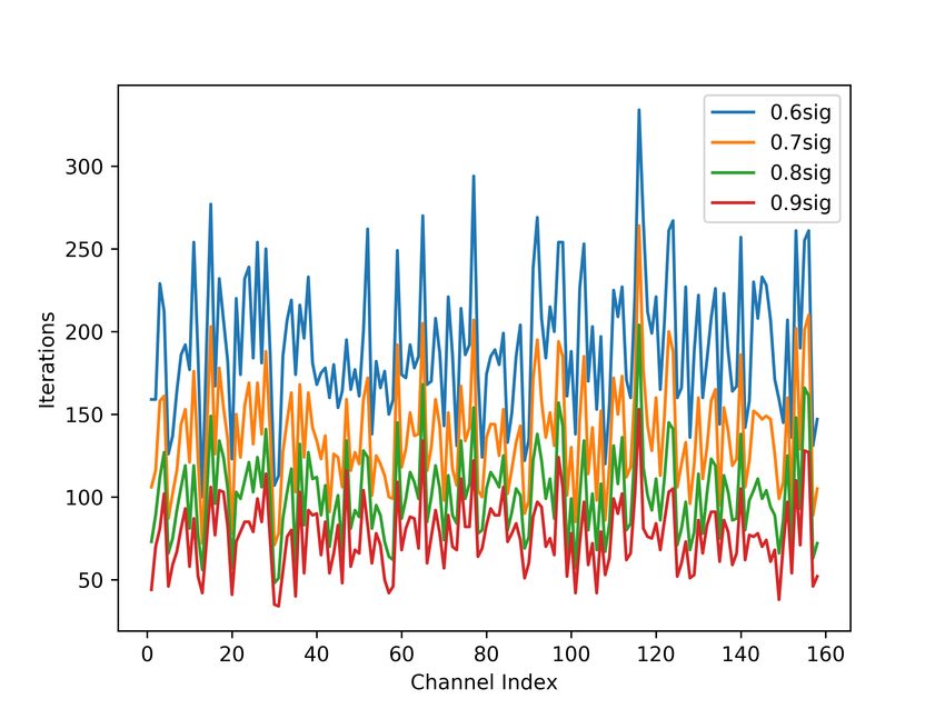
Cubelet Stacking                  3
PSFs were assumed to be identical to the PSFs calculated from the              (ii) The frequency axes from the different spectra are now mis-
above uv-coverage, after flagging. No signal data is used in this                  aligned, so we linearly interpolate each spectrum to a pre-
                                                                                                                        interp              interp
paper, but noise from signal-free portions of the data is used to                                             0
                                                                                   defined frequency array ( fk,l −−−−→ Fk,l , s0A,k,l −−−−→ s00A,k,l ) prior
conduct the simulation.                                                            to stacking. The channel spacing of the pre-defined array is
      Optical redshift data for the simulation were based on the                   62.5 kHz.
internal version of GAMA DR3 catalogue (Baldry et al. 2018),
choosing only those redshifts that overlap with the frequency range
of the VLA data cubes. Only galaxies with redshift robustness                 (iii) The flux densities for spectra not extracted from the centre of
NQ > 2 are selected. After cross-matching, together with addi-                     the primary beam need to be corrected for primary beam at-
tional considerations (the galaxy not being too close to the fre-                  tenuation: S A,k,l = s00A,k,l /pl , where p is the VLA primary beam
quency or spatial edges of data cubes, and the galaxy being within                 response for a given galaxy offset.
the primary beam), this results in an input stacking catalogue of
3622 galaxies. Within the 267 VLA pointings, these 3622 galax-
ies result in 5442 independent spectra and image cubelets, as some             (iv) The rms noise for each channel in each spectrum is calcu-
of the galaxies are located at edge of several pointings and hence                 lated from regions in the corresponding image plane without
observed more than once.                                                           any emission. The rms noise array is represented as σk,l .

                                                                                     At this point we stack the spectra, where the stacked spectrum
                                                                             S 0A,k is:
3     STACKING METHODOLOGY                                                              P
                                                                                          S A,k,l wk,l
                                                                             S 0A,k = lP               ,                                         (1)
In this section, we summarize the methodology of the traditional                            l wk,l
H i spectral stacking method and introduce the technique of cubelet          where w denotes the weight assigned to each spectrum and spectral
stacking. For normal spectral stacking, individual spectra are first         channel. In this paper, we use weight factors which relate only to
extracted from data cubes based on their optical 3D coordinates              primary-beam corrected noise levels and luminosity distances:
(i.e. position and redshift). Then a weighted averaging process is
                                                                             wk,l = σξk,l dlγ .                                                              (2)
applied to these spectra. The weights can take into account the
noise in the data, the distance from the telescope pointing centre           We apply normal noise variance weighting (ξ = −2), but should
and the distance of the galaxies. Using the final stacked spectrum,          also consider differing values for γ, as this choice balances S/N of
the average properties of the galaxy sample, such as flux, H i mass          the stack, the weighted mean redshift of the sample, and the cos-
and linewidth can be studied. Cubelet stacking works in a similar            mic volume probed. γ = 0 corresponds to uniform weighting (e.g.
way, with stacking happening in the image rather than the spectral           Delhaize et al. 2013; Rhee et al. 2013) whereas γ = −1 suppresses
domain - i.e. spectra from a range of positions around the central           noise from high-redshift samples, while not over-biased by low-
position of the galaxies are stacked. However, the PSF cubelets are          redshift galaxies (e.g. Hu et al. 2019). For simplicity, throughout
also extracted and stacked using an identical weighting procedure.           this paper we take γ = 0.
The main benefit of this method is that, when the stacked image                    Although we express the spectral stacking process in flux,
cube has significant S/N ratio, it becomes possible to deconvolve            other kinds of spectra (i.e. in mass, M/L) can be stacked in the
the stacked cube which, as shown in this paper, results in more ac-          same way. In this work we test the method using mass spectra, so
curate image stacks, and flux and mass measurements for resolved             a unit conversion is conducted before the stacking. The conversion
galaxies.                                                                    between H i mass and flux is given by:
                                                                                          !              !2                 !
                                                                                   MH i               DL           FH i
                                                                                            = 49.7                            ,               (3)
                                                                              M beam−1               Mpc     Jy Hz beam−1
3.1    Spectral Stacking
                                                                             where DL is luminosity distance, and FH i is spectrally integrated
From an input optical catalogue with positions and redshifts, we             flux.
define a sample of size N, with subscript l = 1, 2, ..., N indicating
the individual spectra extracted. For a given l-th spectrum, we use
                                                                             3.2    Cubelet Stacking
the subscript k to indicate different frequency channels. The series
of flux densities is denoted sk,l , and the series of corresponding fre-     For every galaxy in this sample, we extract a small image cubelet
quencies is denoted fk,l . The aperture size used for extracting the         from the full dirty cube, centered on its optical position and redshift
spectra is A. This can be an angular area, or physical area. Based           converted into a redshifted H i frequency. We also extract a same-
on whether or not sources are resolved, the aperture can also be             sized PSF cubelet from the full PSF cube, centered on peak of the
chosen as single pixel or an extended area.                                  PSF. The size of extracted cubelets should be big enough to consists
      We first form the spectrum sA,k,l within A. The sA,k,l are in units    most of galaxy signals, and big enough to include main features of
of Jy or Jy/beam, depending on whether the data are spatially in-            PSF, as a deconvolution process will be conducted later.
tegrated or not. However, as noted later, the beam (PSF) size for a               Subscripts for RA, Dec and channels are denoted by i, j, k,
dirty image from an interferometer is not well defined.                      respectively; pixel values in the image cubelet are given by xi, j,k ,
      We apply the following three steps for each spectrum before            pixel values in PSF cubelet by yi, j,k , and the frequency values in
stacking:                                                                    each cubelet are given by fk . We apply the following four steps to
                                                                             the image and PSF cubelet of each galaxy before stacking:
    (i) Blueshift the observed frequency back to the rest frame:
        0
       fk,l = fk,l (1 + zl ). In order to conserve flux, we also apply the      (i) Blueshift the observed frequency axis to the rest frame, and
       cosmological stretch factor: s0A,k,l = sA,k,l /(1 + zl ).                                             0
                                                                                   conserve flux as before: fk,l = fk,l (1+zl ); xi,0 j,k,l = xi, j,k,l /(1+zl ).

MNRAS 000, 1–11 (2021)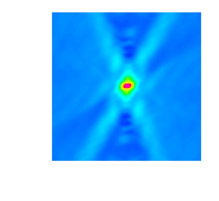
4         Qingxiang Chen et al.
    (ii) Linearly interpolate the frequency axis of the image and
                                                                    interp
                                                       0
        PSF cubelet to a pre-defined frequency array: fk,l −−−−→ Fk,l ;
                 interp                       interp
        xi,0 j,k,l −−−−→ xi,00j,k,l ; yi, j,k,l −−−−→ Yi, j,k,l .

    (iii) Apply primary beam correction: Xi, j,k,l = xi,00j,k,l /pl , where p
         is the VLA primary beam response for a given galaxy offset.

    (iv) We determine the cubelet channel noise σk,l in a similar man-
        ner as for the spectral stacking. The noise is derived using all
        image pixels at a given frequency channel, and not just those
        in the extracted region.

         After applying the above to all spectra in the sample, we stack
both the image cubelets and PSF cubelets. The stacking steps are
similar to spectral stacking, except we now average pixel values in
the image domain and the spectral domain. For the image cubelets,
                                                                                   Figure 1. The distributions of H i galaxy diameters, DH i and Deff predicted
we calculate:
           P                                                                       from scaling relations, for the 3622 GAMA sample. The blue shaded re-
             l Xi, j,k,l wk,l                                                      gion represents the histogram for H i effective diameter. The unfilled red
Xi,0 j,k = P                  .                                      (4)
                l wk,l                                                             histogram shows H i diameters defined by the position where the H i surface
                                                                                   density equals 1 M pc−2 . The vertical dashed line at 1200 represents the
For PSF cubelets, we calculate:
          P                                                                        minor axis of a Gaussian fit to the stacked VLA PSF used in this simula-
            l Yi, j,k,l wk,l                                                       tion.
Yi,0 j,k = P                 ,                                               (5)
               l wk,l

where the weight factors are the same as for spectral stacking.                    Here B, g and r are all absolute magnitudes in the three bands. The
     Note the spectra stacked in these steps can be in flux, mass,                 absolute magnitude of g and r are calculated based on Petrosian
M/L or other kinds. In this work we test our method using mass                     magnitudes, distance moduli, dust extinctions and k-corrections
spectra. The conversion between flux spectrum to mass spectrum is                  provided from Baldry et al. (2018) and Loveday et al. (2012).
in Eq. 3.                                                                               We then take the scaling relation from Dénes et al. (2014) to
     Following stacking, we can then implement deconvolution,                      predict approximate H i masses using:
whereby the stacked image cube X 0 is cleaned under Högbom algo-
rithm with the stacked PSF cube Y 0 . From the deconvolved stacked                 log MH i = 2.89 − 0.34 B.                                               (8)
image cube, a spectrum can then extracted from within a given                      Combining Eq. 8 and the H i size scaling relations in B band from
aperture, and a total flux estimated, taking into account the restor-              Broeils & Rhee (1997), we derive:
ing beam area. Taking the spatial aperture size as A, the clean image
as C, and the Gaussian-fit to the restoring beam from the stacked                  log DH i = 0.4921 log MH i − 3.3766,                                    (9)
PSF as G, we can approximate the spatially integrated spectrum by:                 and
        P                                                                          log Deff = 0.4924 log MH i − 3.5918,                                   (10)
          A C i, j,k
S A,k = P            .                                                       (6)
          A G i, j,k                                                               where DH i is the diameter in kpc where the surface mass density
    Note that A should not exceed the central quarter in the RA-                   drops down to 1 M pc−2 and Deff is the half-mass radius in units of
DEC domain, otherwise the clean algorithm cannot deconvolve the                    kpc. The size distribution of the 3622 GAMA galaxy sample using
PSF from the full cubelet.                                                         scaling relations is shown in Fig 1 after converting these diameters
                                                                                   to angular sizes. In this work we concentrate on the latter definition
                                                                                   (Eq. 10) to represent galaxy H i sizes.
                                                                                         For every galaxy, we take DH i calculated from scaling rela-
4     SIMULATION
                                                                                   tions as the length of the major axis. We take the ellipticity η from
In this section we simulate H i spectral stacking and cubelet stack-               the r-band data to calculate the minor axis b = DH i (1 − η). We
ing to test our method. We use optical scaling relations to simulate               also take the r-band position angle into consideration when sim-
the H i content of the observed galaxy sample and try to recover                   ulating the shape of the galaxies. We then allocate the H i mass
the simulated signal, i.e. average H i mass. In this simulation, we                uniformly to all the voxels occupied by a galaxy, assuming every
concentrate on stacking spectra scaled to mass density units, rather               galaxy has a fixed line-width of 1 MHz. The size for every cubelet
than flux density units.                                                           is 200 pixels × 200 pixels × 160 channels, with the pixel size being
     We first interpolate magnitudes from the GAMA catalogue to                    200 × 200 × 62.5kHz. A line-width of 1 MHz corresponds to 16 chan-
B-band using the SDSS transformation model:2                                       nels in the simulation. Note that the allocated sample size is 5442
                                                                                   rather than 3622, in order to match the real observational sample.
B = g + 0.3130 (g − r) + 0.2271.                                             (7)
                                                                                         We then stack the 5442 models and the PSFs using realis-
                                                                                   tic weight factors wl,k = σ−2 l,k , even in the noise-free simulation.
2  Thanks to Robert Lupton’s work in 2005:                                         The noise information comes from the observed data cubes. This
http://classic.sdss.org/dr4/algorithms/sdssUBVRITransform.html#Lupton2005          makes it consistent with further simulations with noise added. As

                                                                                                                                   MNRAS 000, 1–11 (2021)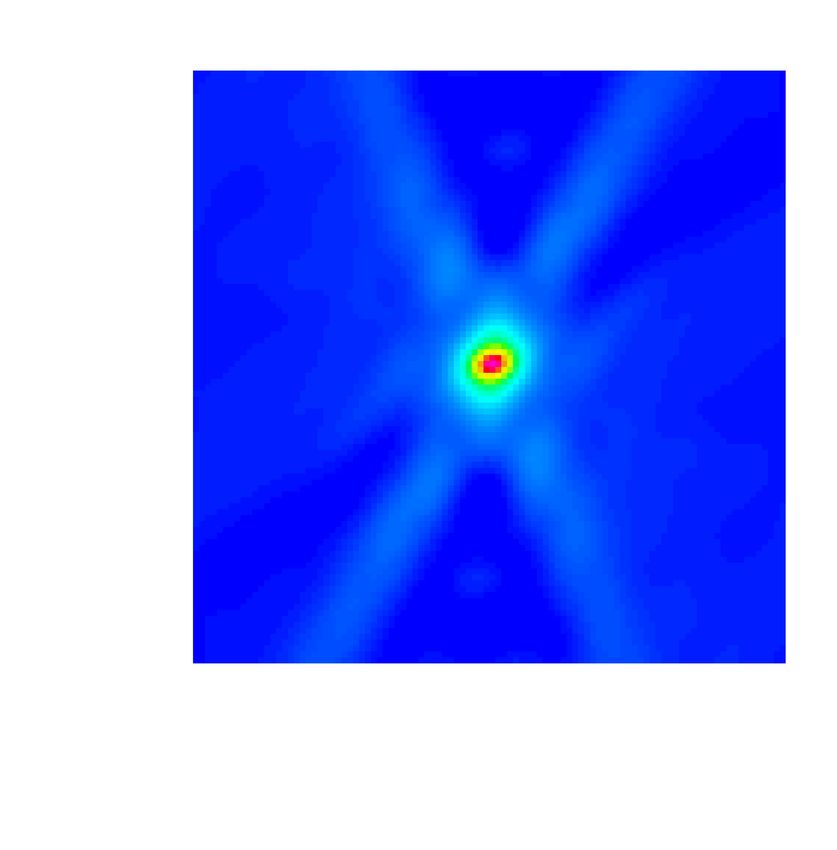
Cubelet Stacking                 5

                                                                              Figure 3. The cumulative H i mass of the stacked model and spectral stack-
                                                                              ing results, as function of aperture size. Of all the H i mass, 99.7% is within
                                                                              2000 radius. The solid, dotted and dashed lines indicate the spectral stacking
                                                                              measurement, model stacking measurement and expected values, respec-
                                                                              tively. Simple application of spectral stacking results in a discrepancy in the
                                                                              measured mass by a factor of 2.3 due to the nature of the psf.

                                                                              4.2     Cubelet Stacking
Figure 2. The stacked model image from the simulation. The model image
for every galaxy is based on the H i mass predicted from the optical magni-   4.2.1    Noise-free cubelet stacking
tudes and colour, and convolved with a top hat model based on the optical
                                                                              For cubelet stacking, we stack in the image domain using Eq. 4, and
position angle and the H i size, also predicted from the optical magnitude.
Noise-based weighting is used in the model stacking, although the image       generate the stacked PSF image cubelet via Eq. 5. After stacking
itself does not include noise. The stacked simulation has an H i mass of      the convolved model images, we deconvolve with the stacked PSF.
1.74 × 10⁹ M . The input images have not been convolved with the PSF.         We use a Högbom clean with a gain of 0.1. We apply 20, 50, 100,
                                                                              200, and 500 iterations respectively to examine clean convergence.

motioned before, we do not consider distance weightings for sim-
plicity. The stacked model image is shown as Fig 2. The stacked H i           4.2.2    Cubelet stacking with noise
mass is 1.74 × 10⁹ M . The curve of growth for the stacked H i mass
                                                                              We add noise to the simulated cubelets in order to better mimic the
distribution (Fig 3) shows that 99.7% of the H i mass is located
                                                                              situation of real observations. For each of the 267 observed point-
within a radius of 2000 .
                                                                              ings, we randomly choose 100 3D positions where no source can
      The next step is to stack the convolved model image cubes,
                                                                              be found in the GAMA catalogue within a distance of 200 pixels
with and without noise, to test whether the above model measure-
                                                                              × 200 pixels × 96 channels (40000 × 40000 × 6 MHz). We then ex-
ments can be reproduced.
                                                                              tract a noise cubelet of size 40000 × 40000 × 10 MHz. We thus obtain
                                                                              26,700 noise cubelets from the 267 fields. We then randomly al-
4.1   Spectral Stacking                                                       locate these noise cubelets to the 5442 image cubelets, repeating
                                                                              the process 20 times, giving 20 noise realisations for each model
In this test, we first convolve the extended models with their actual
                                                                              cubelet. The noise cubelets are then added to the convolved model
observed PSF, to mock an noise free observation. We then stack
                                                                              images, and an identical process of blueshifting, interpolation, pri-
spectra extracted from these convolved images. Pixel units are con-
                                                                              mary beam correction, conversion to mass units, and stacking is
verted from Jy beam−1 to M beam−1 through Eq. 3. A 2D Gaussian
                                                                              followed.
function is fit to each PSF to estimate the beam shape, and spectra
                                                                                    Finally, we deconvolve the stacked image cubelet with the
are extracted by summing up the pixel values in circular area A
                                                                              stacked PSF cubelet. Signal-free channels from the stacked image
from the convolved images. The recovered mass spectrum for each
                                                                              cubelet are used to calculate the rms level, which is then set as the
galaxy is calculated using:
                                                                              cleaning threshold unit. The integrated H i mass is calculated by
         0
MA,k    MA,k G−1
              A,k                                                             integrating within the central 16 signal channels.
     =            .                                                   (11)
M      M beam−1
                    0
In this equation, MA,k is the spectrum extracted from the simulated
image; G A,k is from summing up the values in area A, of the corre-           5     RESULTS
sponding Gaussian PSF approximation normalised to unity at the
                                                                              5.1     Spectral Stacking
central pixel. The extracted spectra are then stacked using Eq. 4.
The final simulated H i mass is then derived by integrating the emis-         The relationship between the measured H i mass and aperture in
sion from the central 16 channels.                                            the case of simple interferometric spectral stacking is shown as the

MNRAS 000, 1–11 (2021)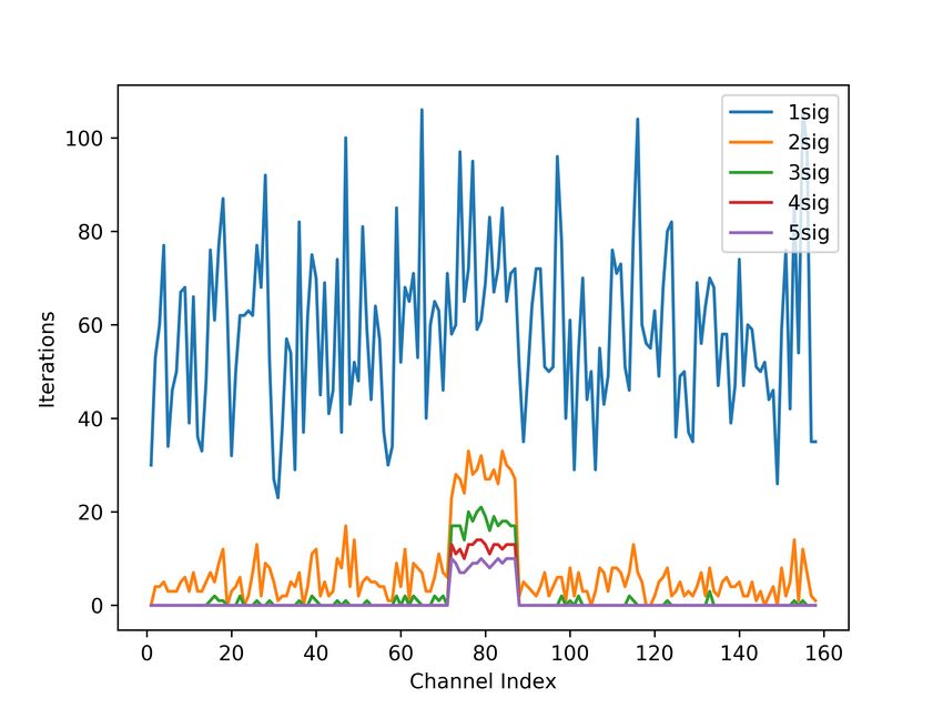
6       Qingxiang Chen et al.
solid line in Fig 3. The measured mass reaches a constant value           For more than 100 iterations, the measured H i mass converges to
at the relatively large radius of ∼8000 . This is much larger than the    the predicted value at large apertures. For less than 50 iterations, the
expected H i galaxy sizes – almost all the gas is expected to be          recovered flux is > 20% too high at our largest measured aperture
located within an aperture of 2000 (see Figs 2 and 3). The maximum        of 6000 . The recovered H i mass for 100 iterations and an aperture
value is 4.06 × 10⁹ M at ∼8200 radius while the predicted value           of 2000 is 1.69 × 10⁹ M , or about 97% of the expected value.
from the scaling relation models is 1.74 × 10⁹ M . Thus, simple
interferometric spectral stacking gives a stacked H i mass which is
overestimated by a factor of 2.3.                                         5.2.2   Cubelet stacking with noise
      This discrepancy arises from the combination of non-Gaussian        We now make 20 realisations of noise using the method described
beams, poor uv-coverage and extended emission. Since the spec-            in Section 4.2.2. As with the noise-free case, we use the standard
tral stacks are not deconvolved, spatial integration will give an in-     CASA task deconvolve with a loop gain of 0.1. We also apply our a
correct integral when the normal assumption of Gaussian beam is           priori expectation of the source properties via a clean mask of 2000
made. The trend for H i mass to continue to increase at R > 2000          radius, and multi-scale components at 6 pixel and 12 pixel (1200 and
is due to sidelobes in two ways. First, there is no clean step, so        2400 , respectively).
sidelobes contaminate the measured curve. Second, as can be seen                 For a typical noise realisation with a clean depth varying be-
from Fig 4(b), the sidelobes extend to a large radii even at the 10%      tween 1 and 5-σ, the number of iterations is shown in Fig 6. Even a
level.                                                                    deep clean down to the 1-σ level doesn’t quite reach the 100 itera-
      This implies, that for interferometric stacking of spectral data,   tions suggested by the noise-free simulation. However, considering
the wrong value for H i mass will be obtained if the interferome-         that we can fix the spatial integration radius at 2000 radius, the sen-
ter resolves the galaxies being observed, unless the interferometer       sitivity to the clean threshhold should be minor (see Fig 5).
beam is very clean (for example Gaussian). The predicted VLA                     The moment 0 image of the central 16 channels is shown be-
beam in this simulation is highly non-Gaussian, partly reflecting         fore and after 1-σ cleaning in Fig 7. The sidelobes are visibly re-
the nature of the VLA baseline distribution, but not helped by the        moved and image quality is dramatically improved. As a function
equatorial placement of the field being simulated. Fig 4(b) is a typ-     of aperture size, the average trend over the 20 realisations is shown
ical PSF image, from the central channel of PSF cube for field 231        in Fig 8 (the Appendix shows the behaviour of the individual re-
(one pointing out of the 267 simulated). As extensively discussed in      alisations). As with the noise-free simulations, all the flux is accu-
Jorsater & van Moorsel (1995), the flux of an extended source can         rately recovered at a 2000 radius aperture. Greater than that aperture,
be easily overestimated by a large factor if it is measured directly      there is gradual rise in the recovered H i mass, resulting in an over-
from dirty images. This is because of poor uv-coverage leading to         estimate of ∼20% at the largest measured aperture of 6000 . This is
highly non-Gaussian PSFs.                                                 similar to the results of the noise-free simulation when the decon-
                                                                          volution is imperfect (< 100 clean iterations).
5.2     Cubelet Stacking                                                         This demonstrates that flux can be recovered from decon-
                                                                          volved stacks even in the presence of noise. Deeper cleaning down
A key motivation for cubelet stacking is improvement of PSF qual-         to 0.6 the rms level was also tested. Fig 9 shows the number of
ity. As above, upper panels in Fig 4 demonstrate how poor PSF             clean iterations as a function of channel index (frequency) and
quality for a short equatorial VLA observation can be, and how            clean depth. At 0.7-σ, where the average number of iterations ex-
much improvement can be made after stacking. Stacking PSFs is             ceeds 100, the flux–aperture relation, as with the noise-free simu-
equivalent to gaining uv-coverage in the normal manner via Earth-         lations, flattens out (see Fig 10). However, there is very little dif-
rotation synthesis. The stacking procedure concentrates the PSF,          ference in the result at 2000 . For the 1-σ threshhold, the H i mass
and suppresses sidelobes.                                                 enclosed within a radius of 2000 is (1.72 ± 0.08) × 109 M , about
      Moreover, assuming that a detection is made after the stacking      only 4% of error around the actual value.
procedure, the stacked image can also be deconvolved. For interfer-
ometric stacking, where the galaxies may be partially resolved, this
procedure mitigates against the effects of sidelobes on the final re-
                                                                          6   DISCUSSION
sult as demonstrated above. For the purposes of deconvolution, we
use the standard CASA task deconvolve, using a loop gain of 0.1.          Interferometers have several advantages over single-dishes for
                                                                          stacking experiments. Firstly, it is often easier to reach thermal
                                                                          noise due to better immunity from systematic problems such as
5.2.1    Noise-free cubelet stacking
                                                                          radio-frequency interference, standing waves, and gain variations.
The moment 0 images of the cubelet stacks, both before and af-            Secondly, angular resolution is usually superior, thus minimising
ter deconvolution, are shown in Fig 4. Both are extracted from the        problems that arise due to source confusion. However, the increased
central 16 channels where H i model data exist. In the right panel,       angular resolution often means that sources will be resolved, which
100 clean iterations are used. The result clearly demonstrates that,      in turn makes it difficult to estimate fluxes from dirty images. In
despite the statistical nature of the stacks, the end result is that      fact, instruments where successful stacking experiments have been
sidelobes are very effectively suppressed and a relatively good 2-        performed, such as GMRT and the VLA, have poor uv-coverage
d Gaussian image is recovered. There are pathological cases where         and highly non-Gaussian PSFs. These successful stacking exper-
such a technique will not work, but for a large number of objects,        iments rely on lowering the resolution (by uv-tapering) to make
this simulation demonstrates that deconvolution of a stack is almost      those extended sources unresolved.
as good as for a single noise-free unstacked image.                             The traditional stacking technique is to extract spectra from
      The derived H i mass as a function of apertures in is shown         a galaxy’s 2-d position and then stack the frequency-shifted spec-
in Fig 5. With a 2000 radius circular aperture, all the flux is recov-    tra. We have introduced a new method for stacking, the so-called
ered. However, the clean depth is important for larger apertures.         cubelet stacking technique. In cubelet stacking the dirty images as

                                                                                                                        MNRAS 000, 1–11 (2021)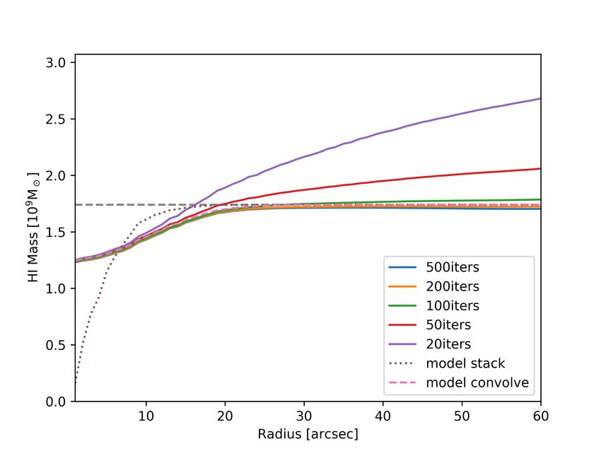
Cubelet Stacking                7

                                   (a) Stacked PSF                                                 (b) Typical PSF without stacking

                               (c) Stacked dirty image                                          (d) Stacked image after deconvolution
Figure 4. Upper: the PSF before and after stacking. (a): the stacked rest-frame PSF for 5442 individual PSFs. (b): a PSF image from a typical observation
pointing (field 231) at the central channel. The colour scales of the two images are identical. The contour levels from the centre outwards are 0.5, 0.2 and 0.1
respectively. The four surrounding sidelobes are also contoured at the 0.1 level. Due to the short integration time at each pointing, the PSF for every cubelet
shows high sidelobes. After the stacking, the PSF becomes more concentrated, with lower sidelobes. Bottom: moment 0 images before and after deconvolution
in a noise-free simulation. (c): the dirty moment 0 image from stacking the convolved model images. (d): the moment 0 map of the restored image after a 100
iterations of clean deconvolution. The two images have the same colour scale. The sidelobes are highly suppressed.

well as their point spread functions are stacked. The main advan-                  equatorial GAMA 9-hr field. The combination of spatially resolved
tages are:                                                                         galaxies, and poor uv-coverage makes it difficult to apply the tradi-
     1. The stacked cubelets can be deconvolved, whereas the indi-                 tional spectral stacking method, as the conversion from Jy/beam to
vidual cubelets cannot.                                                            Jy is only straightforward for unresolved sources in dirty images. It
                                                                                   is otherwise scale-dependent, in which case a Gaussian-like beam
     2. uv-coverage can be improved if many fields are observed                    must be provided. These properties, however, make DINGO-VLA
over a significant length of time (as is the case in our simulation).              ideal for testing the viability of cubelet stacking. Success with this
This results in an improved PSF stack, and better deconvolution.                   data set suggests that cubelet stacking will likely be much more
     The method has been tested using a realistic simulation with                  generally applicable.
actual noise from the DINGO-VLA survey (Chen et al. (prep)).
This survey consists of 267 individual (∼28 min) pointings in the                        The simulation uses the same 5442 cubelet sample as defined

MNRAS 000, 1–11 (2021)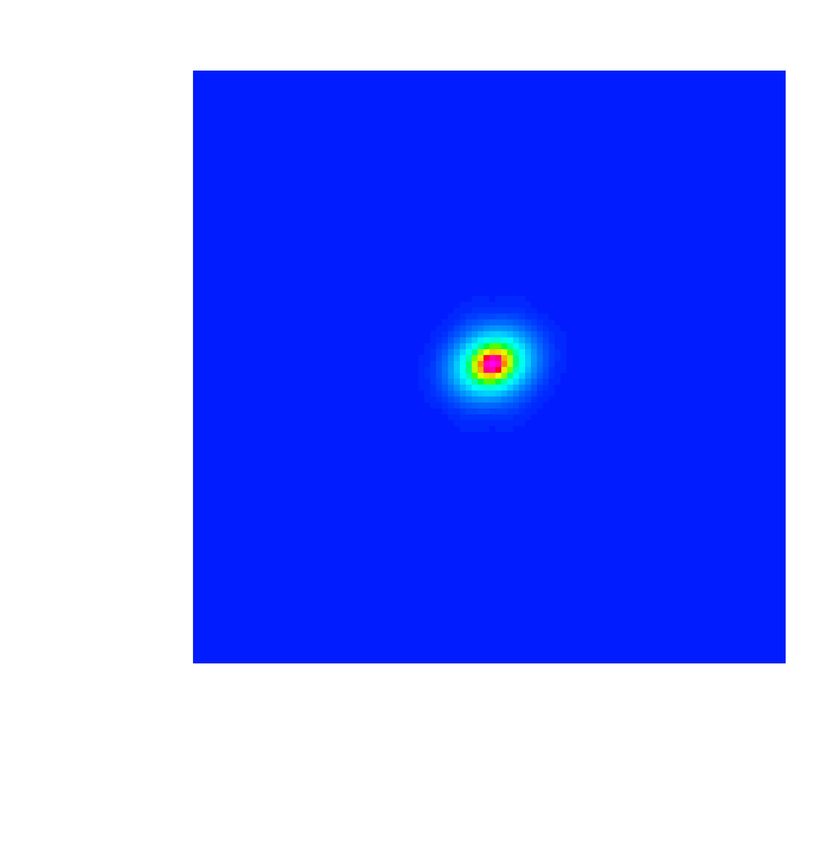
8      Qingxiang Chen et al.
                                                                                tral stacking technique and show that the H i mass is overestimated
                                                                                by a factor of 2.3.
                                                                                      We then simulate the cubelet stacking and deconvolution in
                                                                                two ways. In the noise-free simulation, we stack the convolved
                                                                                cubelets, then deconvolve with the stacked PSF. The sidelobes in
                                                                                the dirty image are highly suppressed. With a clean that is suffi-
                                                                                ciently deep (around 100 iterations in this simulation), the actual
                                                                                value of H i mass is perfectly recovered, proving that in principle
                                                                                this method works. Cubelet stacking can reproduce the correct flux
                                                                                for a spatially extended stack, even where the individual PSFs are
                                                                                irregular and non-Gaussian.
                                                                                      We also conduct simulations with 20 different noise realisa-
                                                                                tions, similar to the actual DINGO-VLA observational project. We
                                                                                randomly generate 20 sets of noise cubelets from parts of our data
                                                                                cubes known not to contain any emission, or catalogued galaxies,
                                                                                We add to the convolved cubelets, then stack. We use a multi-scale
                                                                                deconvolution technique, with a clean mask over the central 2000 ra-
                                                                                dius. This allows us to apply a deep clean where the sidelobes can
Figure 5. Integrated mass as a function of aperture size for the noise-free     be effectively suppressed. The integrated H i mass can be recovered
simulation. The clean gain is 0.1. The five solid curves are the H i masses     with small uncertainty at an aperture radius of ∼2000 .
derived with different numbers of clean cycles. The dotted curve is the ex-           Being able to deconvolve stacks can be especially useful
pected H i mass generated from the stacked model image, which converges
                                                                                where stacked structure matters. For example, it should be possible
to 1.74 × 10⁹ M at a radius of ∼2000 (this value is also indicated by the
                                                                                to align galaxies along the optical major axis to study the stacked
dashed horizontal line). The dashed curve is a similar result, after convolv-
ing the stacked model directly with the Gaussian beam similar in size to the    H i diameter, and hence the relation between MH I and DH I as a
central part of the the stacked PSF. For a successful deconvolution, at least   function of redshift. With this technique the sidelobes of stacked
100 iterations are needed for this noise-free simulation.                       flux in the image domain are cleaned out, enabling the detailed
                                                                                study of flux distributions.
                                                                                      For some stacking projects that observe very large sky areas to
                                                                                avoid cosmic variance, the limited observing time on single point-
                                                                                ings will result in bad uv-coverage. In this case it is impossible
                                                                                to carry out traditional stacking analysis unless sources are unre-
                                                                                solved. But for cubelet stacking, only the combined uv-coverage
                                                                                matters. This allows observers to choose observing a large FoV
                                                                                while still able to apply a stacking analysis.

                                                                                ACKNOWLEDGEMENTS
                                                                                Parts of this research were supported by the Australian Research
                                                                                Council Centre of Excellence for All Sky Astrophysics in 3 Di-
                                                                                mensions (ASTRO 3D), through project number CE170100013,
                                                                                and by the Australian Research Council Centre of Excellence
                                                                                for All-sky Astrophysics (CAASTRO), through project number
                                                                                CE110001020.

Figure 6. The number of clean iterations as a function of channel index (i.e.   DATA AVAILABILITY
frequency) for clean depths between 1 and 5-σ. Model flux only exists in
the 16 channels between 71 and 86. The clean depth is calculated using the      As described in Section 2, the simulations presented in this pa-
rms calculated in the model free channels. This result is typical of the 20     per are modelled after data from the DINGO-VLA and GAMA
noise realisations. For the 1-σ case, channels with and without signal have     surveys. The raw DINGO-VLA data is available from the on-line
similar numbers of iterations.                                                  NRAO data archive3 under projects VLA/14B-315 and VLA/16A-
                                                                                341. The data for the GAMA G09 field is available from the project
                                                                                website4 .
in the DINGO-VLA survey . We firstly used scaling relations to
approximate the H i sizes, shapes and masses of galaxies contained
within the survey. We allocate the flux uniformly to all the pixels             REFERENCES
in 16 channels (1 MHz) of frequency. The use of top-hat distri-                 Baldry I. K., et al., 2018, MNRAS, 474, 3875
bution assumption should lead to conservative conclusions, as it
populates the flux to more outskirts than reality (see discussions in
Appendix B). We then convolve every model image with the corre-                 3   science.nrao.edu/facilities/vla/archive
sponding PSF. Using this sample, we firstly apply the normal spec-              4   www.gama-survey.org

                                                                                                                               MNRAS 000, 1–11 (2021)
Cubelet Stacking                 9

Figure 7. The moment 0 image before and after deconvolution for a typical noise realisation (#19). Left: the dirty moment 0 image from stacking the
convolved model images. Right: the restored moment 0 image after 1-σ cleaning. The deconvolution uses a circular cleaning mask of radius 2000 , and a
multi-scale algorithm. The two plots have identical colour scales. In this simulation, the sidelobes are effectively suppressed and image quality is improved
dramatically.

Figure 8. Integrated mass versus aperture size using a 1-σ threshold clean.       Figure 9. Number of iterations as a function of channel index (frequency)
The horizontal line is the average input mass (1.74 × 10⁹ M ). The solid          for a typical noise realisation, for clean depths from 0.6 to 0.9-σ. In general,
curve show the mean value for the 20 noise realisations. The shaded regions       a depth of at least 0.7-σ is required to reach 100 iterations.
enclose 68% and 95% of the realisations. At an aperture size above ∼2000
radius, the integrated masses tend to grow mildly compared with the input
value, but within the errors.                                                     Brown T., Catinella B., Cortese L., Kilborn V., Haynes M. P., Giovanelli R.,
                                                                                      2015, Monthly Notices of the Royal Astronomical Society, 452, 2479
                                                                                  Brown T., Cortese L., Catinella B., Kilborn V., 2017, Monthly Notices of
Barnes D. G., et al., 2001, MNRAS, 322, 486                                           the Royal Astronomical Society, 473, 1868
Bera A., Kanekar N., Weiner B. J., Sethi S., Dwarakanath K. S., 2018, ApJ,        Catinella B., Haynes M. P., Giovanelli R., Gardner J. P., Connolly A. J.,
    865, 39                                                                           2008, The Astrophysical Journal, 685, L13
Bera A., Kanekar N., Chengalur J. N., Bagla J. S., 2019, ApJ, 882, L7             Crighton N. H. M., et al., 2015, MNRAS, 452, 217
Bird S., Garnett R., Ho S., 2016, Monthly Notices of the Royal Astronomi-         Delhaize J., Meyer M. J., Staveley-Smith L., Boyle B. J., 2013, Monthly
    cal Society, 466, 2111                                                            Notices of the Royal Astronomical Society, 433, 1398
Broeils A. H., Rhee M. H., 1997, A&A, 324, 877                                    Dénes H., Kilborn V. A., Koribalski B. S., 2014, MNRAS, 444, 667

MNRAS 000, 1–11 (2021)
10 Qingxiang Chen et al.
Lanzetta K. M., Wolfe A. M., Turnshek D. A., Lu L., McMahon R. G.,
Hazard C., 1991, ApJS, 77, 1
Li D., Goldsmith P. F., 2003, ApJ, 585, 823
Loveday J., et al., 2012, MNRAS, 420, 1239
Madau P., Dickinson M., 2014, ARA&A, 52, 415
Meyer M., 2009, in Panoramic Radio Astronomy: Wide-field 1-2 GHz Re-
search on Galaxy Evolution. p. 15 (arXiv:0912.2167)
Meyer M. J., et al., 2004, MNRAS, 350, 1195
Meyer M., Robotham A., Obreschkow D., Westmeier T., Duffy A. R.,
Staveley-Smith L., 2017, Publ. Astron. Soc. Australia, 34, 52
Nan R., et al., 2011, International Journal of Modern Physics D, 20, 989
Neeleman M., Prochaska J. X., Ribaudo J., Lehner N., Howk J. C., Rafelski
M., Kanekar N., 2016, ApJ, 818, 113
Noterdaeme P., Petitjean P., Ledoux C., Srianand R., 2009, A&A, 505, 1087
Noterdaeme P., et al., 2012, A&A, 547, L1
Oosterloo T., Verheijen M. A. W., van Cappellen W., Bakker L., Heald G.,
Ivashina M., 2009, in Wide Field Astronomy & Technology for
the Square Kilometre Array. p. 70 (arXiv:0912.0093)
Prochaska J. X., Herbert-Fort S., Wolfe A. M., 2005, ApJ, 635, 123
Rao S. M., Turnshek D. A., Nestor D. B., 2006, ApJ, 636, 610
Figure 10. Integrated mass versus aperture size using a 0.7-σ threshold Rao S. M., Turnshek D. A., Sardane G. M., Monier E. M., 2017, MNRAS,
clean. The horizontal line is the average input mass (1.74 × 10⁹ M ). The 471, 3428
solid curve show the mean value for the 20 noise realisations. The shaded Rhee J., Zwaan M. A., Briggs F. H., Chengalur J. N., Lah P., Oosterloo T.,
regions enclose 68% and 95% of the realisations. At an aperture size above van der Hulst T., 2013, MNRAS, 435, 2693
∼2000 radius, the integrated masses tend to grow mildly compared with the Rhee J., Lah P., Chengalur J. N., Briggs F. H., Colless M., 2016, MNRAS,
input value, but within the errors. 460, 2675
Rhee J., Lah P., Briggs F. H., Chengalur J. N., Colless M., Willner S. P.,
Ashby M. L. N., Le Fèvre O., 2018, MNRAS, 473, 1879
Duffy A. R., Battye R. A., Davies R. D., Moss A., Wilkinson P. N., 2008, Songaila A., Cowie L. L., 2010, ApJ, 721, 1448
MNRAS, 383, 150 Verheijen M., van Gorkom J. H., Szomoru A., Dwarakanath K. S., Poggianti
Duffy A. R., Moss A., Staveley-Smith L., 2012a, Publ. Astron. Soc. Aus- B. M., Schiminovich D., 2007, ApJ, 668, L9
tralia, 29, 202 Wong O. I., et al., 2006, MNRAS, 371, 1855
Duffy A. R., Meyer M. J., Staveley-Smith L., Bernyk M., Croton D. J., Zafar T., Popping A., Péroux C., 2013, A&A, 556, A140
Koribalski B. S., Gerstmann D., Westerlund S., 2012b, MNRAS, 426, Zwaan M. A., van Dokkum P. G., Verheijen M. A. W., 2001, Science, 293,
3385 1800
Fabello S., Kauffmann G., Catinella B., Giovanelli R., Haynes M. P., Heck-
man T. M., Schiminovich D., 2011a, arXiv e-prints, p. arXiv:1104.0414
Fabello S., Catinella B., Giovanelli R., Kauffmann G., Haynes M. P., Heck-
man T. M., Schiminovich D., 2011b, Monthly Notices of the Royal
APPENDIX A: INTEGRATED MASS VS H I MASS FROM
Astronomical Society, 411, 993 DIFFERENT NOISE REALISATIONS
Fabello S., Kauffmann G., Catinella B., Li C., Giovanelli R., Haynes M. P., We attach the mass - aperture relation after deconvolution using a
2012, MNRAS, 427, 2841
2-5σ threshold for all the 20 noise realisations in Fig A1.
Fernández X., et al., 2013, The Astrophysical Journal, 770, L29
Fernández X., et al., 2016, The Astrophysical Journal, 824, L1
Freudling W., et al., 2011, ApJ, 727, 40
Geréb K., Morganti R., Oosterloo T. A., Guglielmino G., Prandoni I., 2013, APPENDIX B: EXPONENTIAL AND TOP-HAT MODELS
A&A, 558, A54
Giovanelli R., et al., 2005, AJ, 130, 2598 We compare top hat and exponential models for the distribution of
Haynes M. P., et al., 2018, The Astrophysical Journal, 861, 49 H i surface density. The exponential model is defined by
Holwerda B. W., Blyth S. L., Baker A. J., 2012, in Tuffs R. J., Popescu r
C. C., eds, IAU Symposium Vol. 284, The Spectral Energy Distri- Σ(r) = Σ0 exp (− ), (B1)
r0
bution of Galaxies - SED 2011. pp 496–499 (arXiv:1109.5605),
doi:10.1017/S1743921312009702 where the total mass is given by
Hopkins A. M., Beacom J. F., 2006, ApJ, 651, 142 MH I
Hoppmann L., Staveley-Smith L., Freudling W., Zwaan M. A., Minchin Σ0 = . (B2)
2πr02
R. F., Calabretta M. R., 2015, Monthly Notices of the Royal Astronom-
ical Society, 452, 3726 From the previous definition of DH I we solve for r0 given MH I
Hu W., et al., 2019, Monthly Notices of the Royal Astronomical Society, and Σ(RH I ) = 1 M /pc2 for each of the 3622 simulated GAMA
489, 1619 galaxies, and determine each of the surface density profiles. The
Johnston S., et al., 2008, Experimental Astronomy, 22, 151 integrated MH I profiles for both the exponential and top-hat models
Jones M. G., Papastergis E., Haynes M. P., Giovanelli R., 2015, MNRAS,
for a galaxy with MH I = 109 M is shown in Fig B1. The shapes of
449, 1856
profiles change only marginally at MH I values between 107 M and
Jones M. G., Haynes M. P., Giovanelli R., Papastergis E., 2016, MNRAS,
455, 1574 1010 M . For the exponential model, the radii that enclose 50% and
Jorsater S., van Moorsel G. A., 1995, AJ, 110, 2037 80% of MH I are 37% and 65% of RH I . For the top hat model, the
Kanekar N., Sethi S., Dwarakanath K. S., 2016, ApJ, 818, L28 corresponding values are 71% and 90% of RH I . The top hat model,
Lah P., et al., 2007, MNRAS, 376, 1357 whilst not as realistic as the exponential model, represents a more
Lah P., et al., 2009, MNRAS, 399, 1447 challenging ‘worst-case’ scenario.
MNRAS 000, 1–11 (2021)Cubelet Stacking 11
Figure A1. Similar to Fig 8, the integrated mass versus aperture size using 2, 3, 4 and 5-σ thresholds for clean. The horizontal line is the average input mass
(1.74 × 10⁹ M ). The solid curve show the mean value for the 20 noise realisations. The shaded regions enclose 68% and 95% of the realisations.
This paper has been typeset from a TEX/LATEX file prepared by the author.
Figure B1. The integrated mass profiles from exponential and top-hat mod-
els for galaxy with MH I = 109 M . The right hand y-axis is the percentage
of the enclosed mass relative to the total MH I .
MNRAS 000, 1–11 (2021)You can also read