Interpretable Machine Learning: Fundamental Principles and 10 Grand Challenges
←
→
Page content transcription
If your browser does not render page correctly, please read the page content below

Interpretable Machine Learning: Fundamental
                                                          Principles and 10 Grand Challenges
                                         Cynthia Rudin1 , Chaofan Chen2 , Zhi Chen1 , Haiyang Huang1 , Lesia Semenova1 ,
                                                                      and Chudi Zhong1
arXiv:2103.11251v2 [cs.LG] 10 Jul 2021

                                                                                        1
                                                                                         Duke University
                                                                                    2
                                                                                        University of Maine

                                                                                            July, 2021

                                                                                              Abstract
                                                       Interpretability in machine learning (ML) is crucial for high stakes decisions and trou-
                                                  bleshooting. In this work, we provide fundamental principles for interpretable ML, and dispel
                                                  common misunderstandings that dilute the importance of this crucial topic. We also identify
                                                  10 technical challenge areas in interpretable machine learning and provide history and back-
                                                  ground on each problem. Some of these problems are classically important, and some are
                                                  recent problems that have arisen in the last few years. These problems are: (1) Optimizing
                                                  sparse logical models such as decision trees; (2) Optimization of scoring systems; (3) Placing
                                                  constraints into generalized additive models to encourage sparsity and better interpretability;
                                                  (4) Modern case-based reasoning, including neural networks and matching for causal infer-
                                                  ence; (5) Complete supervised disentanglement of neural networks; (6) Complete or even par-
                                                  tial unsupervised disentanglement of neural networks; (7) Dimensionality reduction for data
                                                  visualization; (8) Machine learning models that can incorporate physics and other generative
                                                  or causal constraints; (9) Characterization of the “Rashomon set” of good models; and (10)
                                                  Interpretable reinforcement learning. This survey is suitable as a starting point for statisticians
                                                  and computer scientists interested in working in interpretable machine learning.1

                                         Introduction
                                         With widespread use of machine learning (ML), the importance of interpretability has become
                                         clear in avoiding catastrophic consequences. Black box predictive models, which by definition are
                                         inscrutable, have led to serious societal problems that deeply affect health, freedom, racial bias, and
                                         safety. Interpretable predictive models, which are constrained so that their reasoning processes are
                                         more understandable to humans, are much easier to troubleshoot and to use in practice. It is uni-
                                         versally agreed that interpretability is a key element of trust for AI models (Wagstaff, 2012; Rudin
                                            1
                                                Equal contribution from C. Chen, Z. Chen, H. Huang, L. Semenova, and C. Zhong

                                                                                                  1
and Wagstaff, 2014; Lo Piano, 2020; Ashoori and Weisz, 2019; Thiebes et al., 2020; Spiegelhalter,
2020; Brundage et al., 2020). In this survey, we provide fundamental principles, as well as 10
technical challenges in the design of inherently interpretable machine learning models.
     Let us provide some background. A black box machine learning model is a formula that is
either too complicated for any human to understand, or proprietary, so that one cannot understand
its inner workings. Black box models are difficult to troubleshoot, which is particularly problem-
atic for medical data. Black box models often predict the right answer for the wrong reason (the
“Clever Hans” phenomenon), leading to excellent performance in training but poor performance
in practice (Schramowski et al., 2020; Lapuschkin et al., 2019; O’Connor, 2021; Zech et al., 2018;
Badgeley et al., 2019; Hamamoto et al., 2020). There are numerous other issues with black box
models. In criminal justice, individuals may have been subjected to years of extra prison time due
to typographical errors in black box model inputs (Wexler, 2017) and poorly-designed proprietary
models for air quality have had serious consequences for public safety during wildfires (McGough,
2018); both of these situations may have been easy to avoid with interpretable models. In cases
where the underlying distribution of data changes (called domain shift, which occurs often in prac-
tice), problems arise if users cannot troubleshoot the model in real-time, which is much harder with
black box models than interpretable models. Determining whether a black box model is fair with
respect to gender or racial groups is much more difficult than determining whether an interpretable
model has such a bias. In medicine, black box models turn computer-aided decisions into auto-
mated decisions, precisely because physicians cannot understand the reasoning processes of black
box models. Explaining black boxes, rather than replacing them with interpretable models, can
make the problem worse by providing misleading or false characterizations (Rudin, 2019; Laugel
et al., 2019; Lakkaraju and Bastani, 2020), or adding unnecessary authority to the black box (Rudin
and Radin, 2019). There is a clear need for innovative machine learning models that are inherently
interpretable.
     There is now a vast and confusing literature on some combination of interpretability and ex-
plainability. Much literature on explainability confounds it with interpretability/comprehensibility,
thus obscuring the arguments (and thus detracting from their precision), and failing to convey the
relative importance and use-cases of the two topics in practice. Some of the literature discusses
topics in such generality that its lessons have little bearing on any specific problem. Some of
it aims to design taxonomies that miss vast topics within interpretable ML. Some of it provides
definitions that we disagree with. Some of it even provides guidance that could perpetuate bad
practice. Importantly, most of it assumes that one would explain a black box without consideration
of whether there is an interpretable model of the same accuracy. In what follows, we provide some
simple and general guiding principles of interpretable machine learning. These are not meant to
be exhaustive. Instead they aim to help readers avoid common but problematic ways of thinking
about interpretability in machine learning.
     The major part of this survey outlines a set of important and fundamental technical grand
challenges in interpretable machine learning. These are both modern and classical challenges,
and some are much harder than others. They are all either hard to solve, or difficult to formulate
correctly. While there are numerous sociotechnical challenges about model deployment (that can
be much more difficult than technical challenges), human-computer-interaction challenges, and
how robustness and fairness interact with interpretability, those topics can be saved for another day.
We begin with the most classical and most canonical problems in interpretable machine learning:
how to build sparse models for tabular data, including decision trees (Challenge #1) and scoring

                                                  2
systems (Challenge #2). We then delve into a challenge involving additive models (Challenge
#3), followed by another in case-based reasoning (Challenge #4), which is another classic topic
in interpretable artificial intelligence. We then move to more exotic problems, namely supervised
and unsupervised disentanglement of concepts in neural networks (Challenges #5 and #6). Back
to classical problems, we discuss dimension reduction (Challenge #7). Then, how to incorporate
physics or causal constraints (Challenge #8). Challenge #9 involves understanding, exploring, and
measuring the Rashomon set of accurate predictive models. Challenge #10 discusses interpretable
reinforcement learning. Table 1 provides a guideline that may help users to match a dataset to a
suitable interpretable supervised learning technique. We will touch on all of these techniques in
the challenges.

 Models                          Data type
 decision trees / decision lists somewhat clean tabular data with interactions, including mul-
 (rule lists) / decision sets    ticlass problems. Particularly useful for categorical data with
                                 complex interactions (i.e., more than quadratic).
 scoring systems                 somewhat clean tabular data, typically used in medicine and
                                 criminal justice because they are small enough that they can be
                                 memorized by humans.
 generalized additive models continuous data with at most quadratic interactions, useful for
 (GAMs)                          large-scale medical record data.
 case-based reasoning            any data type (different methods exist for different data types),
                                 including multiclass problems.
 disentangled neural networks data with raw inputs (computer vision, time series, textual data),
                                 suitable for multiclass problems.

Table 1: Rule of thumb for the types of data that naturally apply to various supervised learning
algorithms. “Clean” means that the data do not have too much noise or systematic bias. “Tabular”
means that the features are categorical or real, and that each feature is a meaningful predictor of
the output on its own. “Raw” data is unprocessed and has a complex data type, e.g., image data
where each pixel is a feature, medical records, or time series data.

General Principles of Interpretable Machine Learning
Our first fundamental principle defines interpretable ML, following Rudin (2019):

Principle 1 An interpretable machine learning model obeys a domain-specific set of constraints to
allow it (or its predictions, or the data) to be more easily understood by humans. These constraints
can differ dramatically depending on the domain.

     A typical interpretable supervised learning setup, with data {zi }i , and models chosen from
function class F is:
      1X
 min        Loss(f, zi ) + C · InterpretabilityPenalty(f ), subject to InterpretabilityConstraint(f ),
 f ∈F n
         i
                                                                                                  (1)

                                                  3
where the loss function, as well as soft and hard interpretability constraints, are chosen to match
the domain. (For classification zi might be (xi , yi ), xi ∈ Rp , yi ∈ {−1, 1}.) The goal of these
constraints is to make the resulting model f or its predictions more interpretable. While solutions
of (1) would not necessarily be sufficiently interpretable to use in practice, the constraints would
generally help us find models that would be interpretable (if we design them well), and we might
also be willing to consider slightly suboptimal solutions to find a more useful model. The constant
C trades off between accuracy and the interpretability penalty, and can be tuned, either by cross-
validation or by taking into account the user’s desired tradeoff between the two terms.
     Equation (1) can be generalized to unsupervised learning, where the loss term is simply re-
placed with a loss term for the unsupervised problem, whether it is novelty detection, clustering,
dimension reduction, or another task.
     Creating interpretable models can sometimes be much more difficult than creating black box
models for many different reasons including: (i) Solving the optimization problem may be com-
putationally hard, depending on the choice of constraints and the model class F. (ii) When one
does create an interpretable model, one invariably realizes that the data are problematic and require
troubleshooting, which slows down deployment (but leads to a better model). (iii) It might not be
initially clear which definition of interpretability to use. This definition might require refinement,
sometimes over multiple iterations with domain experts. There are many papers detailing these
issues, the earliest dating from the mid-1990s (e.g., Kodratoff, 1994).
     Interpretability differs across domains just as predictive performance metrics vary across do-
mains. Just as we might choose from a variety of performance metrics (e.g., accuracy, weighted
accuracy, precision, average precision, precision@N, recall, recall@N, DCG, NCDG, AUC, par-
tial AUC, mean-time-to-failure, etc.), or combinations of these metrics, we might also choose from
a combination of interpretability metrics that are specific to the domain. We may not be able to
define a single best definition of interpretability; regardless, if our chosen interpretability measure
is helpful for the problem at hand, we are better off including it. Interpretability penalties or con-
straints can include sparsity of the model, monotonicity with respect to a variable, decomposibility
into sub-models, an ability to perform case-based reasoning or other types of visual comparisons,
disentanglement of certain types of information within the model’s reasoning process, generative
constraints (e.g., laws of physics), preferences among the choice of variables, or any other type
of constraint that is relevant to the domain. Just as it would be futile to create a complete list of
performance metrics for machine learning, any list of interpretability metrics would be similarly
fated.
     Our 10 challenges involve how to define some of these interpretability constraints and how
to incorporate them into machine learning models. For tabular data, sparsity is usually part of
the definition of interpretability, whereas for computer vision of natural images, it generally is
not. (Would you find a model for natural image classification interpretable if it uses only a few
pixels from the image?) For natural images, we are better off with interpretable neural networks
that perform case-based reasoning or disentanglement, and provide us with a visual understanding
of intermediate computations; we will describe these in depth. Choices of model form (e.g., the
choice to use a decision tree, or a specific neural architecture) are examples of interpretability
constraints. For most problems involving tabular data, a fully interpretable model, whose full
calculations can be understood by humans such as a sparse decision tree or sparse linear model, is
generally more desirable than either a model whose calculations can only be partially understood,
or a model whose predictions (but not its model) can be understood. Thus, we make a distinction

                                                  4
between fully interpretable and partially interpretable models, often preferring the former.
    Interpretable machine learning models are not needed for all machine learning problems. For
low-stakes decisions (e.g., advertising), for decisions where an explanation would be trivial and the
model is 100% reliable (e.g., “there is no lesion in this mammogram” where the explanation would
be trivial), for decisions where humans can verify or modify the decision afterwards (e.g., segmen-
tation of the chambers of the heart), interpretability is probably not needed.2 On the other hand,
for self-driving cars, even if they are very reliable, problems would arise if the car’s vision sys-
tem malfunctions causing a crash and no reason for the crash is available. Lack of interpretability
would be problematic in this case.
    Our second fundamental principle concerns trust:

Principle 2 Despite common rhetoric, interpretable models do not necessarily create or enable
trust – they could also enable distrust. They simply allow users to decide whether to trust them. In
other words, they permit a decision of trust, rather than trust itself.

    With black boxes, one needs to make a decision about trust with much less information; without
knowledge about the reasoning process of the model, it is much more difficult to detect whether
it might generalize beyond the dataset. As stated by Afnan et al. (2021) with respect to medical
decisions, while interpretable AI is an enhancement of human decision making, black box AI is a
replacement of it.
    An important point about interpretable machine learning models is that there is no scientific
evidence for a general tradeoff between accuracy and interpretability when one considers the full
data science process for turning data into knowledge. (Examples of such pipelines include KDD,
CRISP-DM, or the CCC Big Data Pipelines; see Figure 1, or Fayyad et al. 1996; Chapman et al.
2000; Agrawal et al. 2012.) In real problems, interpretability is useful for troubleshooting, which

         Figure 1: Knowledge Discovery Process (figure adapted from Fayyad et al., 1996)
                                              .

leads to better accuracy, not worse. In that sense, we have the third principle:

Principle 3 It is important not to assume that one needs to make a sacrifice in accuracy in order
to gain interpretability. In fact, interpretability often begets accuracy, and not the reverse. Inter-
   2
    Obviously, this document does not apply to black box formulas that not depend on randomness in the data, i.e., a
calculation of deterministic function, not machine learning.

                                                         5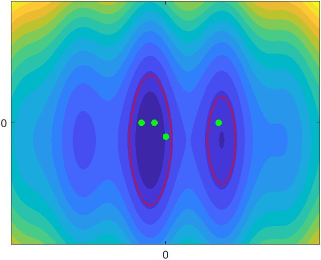
pretability versus accuracy is, in general, a false dichotomy in machine learning.

     Interpretability has traditionally been associated with complexity, and specifically, sparsity, but
model creators generally would not equate interpretability with sparsity. Sparsity is often one com-
ponent of interpretability, and a model that is sufficiently sparse but has other desirable properties
is more typical. While there is almost always a tradeoff of accuracy with sparsity (particularly for
extremely small models), there is no evidence of a general tradeoff of accuracy with interpretabil-
ity. Let us consider both (1) development and use of ML models in practice, and (2) experiments
with static datasets; in neither case have interpretable models proven to be less accurate.

Development and use of ML models in practice. A key example of the pitfalls of black box models
when used in practice is the story of COMPAS (Northpointe, 2013; Rudin et al., 2020). COMPAS
is a black box because it is proprietary: no one outside of its designers knows its secret formula for
predicting criminal recidivism, yet it is used widely across the United States and influences parole,
bail, and sentencing decisions that deeply affect people’s lives (Angwin et al., 2016). COMPAS
is error-prone because it could require over 130 variables, and typographical errors in those vari-
ables influence outcomes (Wexler, 2017). COMPAS has been explained incorrectly, where the
news organization ProPublica mistakenly assumed that an important variable in an approximation
to COMPAS (namely race) was also important to COMPAS itself, and used this faulty logic to
conclude that COMPAS depends on race other than through age and criminal history (Angwin
et al., 2016; Rudin et al., 2020). While the racial bias of COMPAS does not seem to be what
ProPublica claimed, COMPAS still has unclear dependence on race. And worst, COMPAS seems
to be unnecessarily complicated as it does not seem to be any more accurate than a very sparse
decision tree (Angelino et al., 2017, 2018) involving only a couple of variables. It is a key example
simultaneously demonstrating many pitfalls of black boxes in practice. And, it shows an example
of when black boxes are unnecessary, but used anyway.
     There are other systemic issues that arise when using black box models in practice or when
developing them as part of a data science process, that would cause them to be less accurate than
an interpretable model. A full list is beyond the scope of this particular survey, but an article that
points out many serious issues that arise with black box models in a particular domain is that of
Afnan et al. (2021), who discuss in vitro fertilization (IVF). In modern IVF, black box models
that have not been subjected to randomized controlled trials determine who comes into existence.
Afnan et al. (2021) points out ethical and practical issues, ranging from the inability to perform
shared decision-making with patients, to economic consequences of clinics needing to “buy into”
environments that are similar to those where the black box models are trained so as to avoid distri-
bution shift; this is necessary precisely because errors cannot be detected effectively in real-time
using the black box. They also discuss accountability issues (“Who is accountable when the model
causes harm?”). Finally, they present a case where a standard performance metric (namely area
under the ROC curve – AUC) has been misconstrued as representing the value of a model in prac-
tice, potentially leading to overconfidence in the performance of a black box model. Specifically,
a reported AUC was inflated by including many “obvious” cases in the sample over which it was
computed. If we cannot trust reported numerical performance results, then interpretability would
be a crucial remaining ingredient to assess trust.
     In a full data science process, like the one shown in Figure 1, interpretability plays a key role in
determining how to update the other steps of the process for the next iteration. One interprets the

                                                   6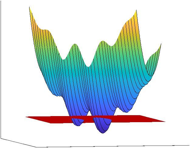
results and tunes the processing of the data, the loss function, the evaluation metric, or anything
else that is relevant, as shown in the figure. How can one do this without understanding how the
model works? It may be possible, but might be much more difficult. In essence, the messiness that
comes with messy data and complicated black box models causes lower quality decision-making
in practice.
    Let’s move on to a case where the problem is instead controlled, so that we have a static dataset
and a fixed evaluation metric.

Static datasets. Most benchmarking of algorithms is done on static datasets, where the data and
evaluation metric are not cleaned or updated as a result of a run of an algorithm. In other words,
these experiments are not done as part of a data science process, they are only designed to compare
algorithms in a controlled experimental environment.
    Even with static datasets and fixed evaluation metrics, interpretable models do not generally
lead to a loss in accuracy over black box models. Even for deep neural networks for computer
vision, even on the most challenging of benchmark datasets, a plethora of machine learning tech-
niques have been designed that do not sacrifice accuracy but gain substantial interpretability
(Zhang et al., 2018; Chen et al., 2019; Koh et al., 2020; Chen et al., 2020; Angelov and Soares,
2020; Nauta et al., 2020b).
    Let us consider two extremes of data types: tabular data, where all variables are real or discrete
features, each of which is meaningful (e.g., age, race, sex, number of past strokes, congestive heart
failure), and “raw” data, such as images, sound files or text, where each pixel, bit, or word is
not useful on its own. These types of data have different properties with respect to both machine
learning performance and interpretability.
    For tabular data, most machine learning algorithms tend to perform similarly in terms of pre-
diction accuracy. This means it is often difficult even to beat logistic regression, assuming one is
willing to perform minor preprocessing such as creating dummy variables (e.g., see Christodoulou
et al., 2019). In these domains, neural networks generally find no advantage. It has been known
for a very long time that very simple models perform surprisingly well for tabular data (Holte,
1993). The fact that simple models perform well for tabular data could arise from the Rashomon
Effect discussed by Leo Breiman (Breiman et al., 2001). Breiman posits the possibility of a large
Rashomon set, i.e., a multitude of models with approximately the minumum error rate, for many
problems. Semenova et al. (2019) show that as long as a large Rashomon set exists, it is more
likely that some of these models are interpretable.
    For raw data, on the other hand, neural networks have an advantage currently over other
approaches (Krizhevsky et al., 2017). In these raw data cases, the definition of interpretability
changes; for visual data, one may require visual explanations. In such cases, as discussed earlier
and in Challenges 4 and 5, interpretable neural networks suffice, without losing accuracy.
    These two data extremes show that in machine learning, the dichotomy between the accurate
black box and the less-accurate interpretable model is false. The often-discussed hypothetical
choice between the accurate machine-learning-based robotic surgeon and the less-accurate human
surgeon is moot once someone builds an interpretable robotic surgeon. Given that even the most
difficult computer vision benchmarks can be solved with interpretable models, there is no reason
to believe that an interpretable robotic surgeon would be worse than its black box counterpart. The
question ultimately becomes whether the Rashomon set should permit such an interpretable robotic
surgeon–and all scientific evidence so far (including a large-and-growing number of experimental

                                                  7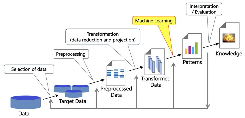
papers on interpretable deep learning) suggests it would.
   Our next principle returns to the data science process.

Principle 4 As part of the full data science process, one should expect both the performance met-
ric and interpretability metric to be iteratively refined.

   The knowledge discovery process in Figure 1 explicitly shows these important feedback loops.
We have found it useful in practice to create many interpretable models (satisfying the known
constraints) and have domain experts choose between them. Their rationale for choosing one
model over another helps to refine the definition of interpretability. Each problem can thus have its
own unique interpretability metrics (or set of metrics).
   The fifth principle is as follows:

Principle 5 For high stakes decisions, interpretable models should be used if possible, rather than
“explained” black box models.

    Hence, this survey concerns the former. This is not a survey on Explainable AI (XAI, where
one attempts to explain a black box using an approximation model, derivatives, variable impor-
tance measures, or other statistics), it is a survey on Interpretable Machine Learning (creating a
predictive model that is not a black box). Unfortunately, these topics are much too often lumped
together within the misleading term “explainable artificial intelligence” or “XAI” despite a chasm
separating these two concepts (Rudin, 2019). Explainability and interpretability techniques are not
alternative choices for many real problems, as the recent surveys often imply; one of them (XAI)
can be dangerous for high-stakes decisions to a degree that the other is not.
    Interpretable ML is not a subset of XAI. The term XAI dates from ∼2016, and grew out of work
on function approximation; i.e., explaining a black box model by approximating its predictions by
a simpler model (e.g., Craven and Shavlik, 1995; Craven, 1996), or explaining a black box using
local approximations. Interpretable ML also has a (separate) long and rich history, dating back to
the days of expert systems in the 1950’s, and the early days of decision trees. While these topics
may sound similar to some readers, they differ in ways that are important in practice.
    In particular, there are many serious problems with the use of explaining black boxes posthoc,
as outlined in several papers that have shown why explaining black boxes can be misleading and
why explanations do not generally serve their intended purpose (Rudin, 2019; Laugel et al., 2019;
Lakkaraju and Bastani, 2020). The most compelling such reasons are:

    • Explanations for black boxes are often problematic and misleading, potentially creating mis-
      placed trust in black box models. Such issues with explanations have arisen with assessment
      of fairness and variable importance (Rudin et al., 2020; Dimanov et al., 2020) as well as un-
      certainty bands for variable importance (Gosiewska and Biecek, 2020; Fisher et al., 2019).
      There is an overall difficulty in troubleshooting the combination of a black box and an ex-
      planation model on top of it; if the explanation model is not always correct, it can be difficult
      to tell whether the black box model is wrong, or if it is right and the explanation model is
      wrong. Ultimately, posthoc explanations are wrong (or misleading) too often.
      One particular type of posthoc explanation, called saliency maps (also called attention maps)
      have become particularly popular in radiology and other computer vision domains despite

                                                  8
known problems (Adebayo et al., 2018; Chen et al., 2019; Zhang et al., 2019). Saliency maps
         highlight the pixels of an image that are used for a prediction, but they do not explain how the
         pixels are used. As an analogy, consider a real estate agent who is pricing a house. A “black
         box” real estate agent would provide the price with no explanation. A “saliency” real estate
         agent would say that the price is determined from the roof and backyard, but doesn’t explain
         how the roof and backyard were used to determine the price. In contrast, an interpretable
         agent would explain the calculation in detail, for instance, using “comps” or comparable
         properties to explain how the roof and backyard are comparable between properties, and
         how these comparisons were used to determine the price. One can see from this real estate
         example how the saliency agent’s explanation is insufficient.
         Saliency maps also tend to be unreliable; researchers often report that different saliency
         methods provide different results, making it unclear which one (if any) actually represents
         the network’s true attention.3

       • Black boxes are generally unnecessary, given that their accuracy is generally not better than a
         well-designed interpretable model. Thus, explanations that seem reasonable can undermine
         efforts to find an interpretable model of the same level of accuracy as the black box.

       • Explanations for complex models hide the fact that complex models are difficult to use in
         practice for many different reasons. Typographical errors in input data are a prime example
         of this issue (as in the use of COMPAS in practice, see Wexler, 2017). A model with 130
         hand-typed inputs is more error-prone than one involving 5 hand-typed inputs.

    In that sense, explainability methods are often used as an excuse to use a black box model–
whether or not one is actually needed. Explainability techniques give authority to black box models
rather than suggesting the possibility of models that are understandable in the first place (Rudin
and Radin, 2019).
    XAI surveys have (thus far) universally failed to acknowledge the important point that inter-
pretability begets accuracy when considering the full data science process, and not the other way
around. Perhaps this point is missed because of the more subtle fact that one does generally lose
accuracy when approximating a complicated function with a simpler one, and these imperfect ap-
proximations are the foundation of XAI. (Again the approximations must be imperfect, otherwise
one would throw out the black box and instead use the explanation as an inherently interpretable
model.) But function approximators are not used in interpretable ML; instead of approximating
a known function (a black box ML model), interpretable ML can choose from a potential myriad
of approximately-equally-good models, which, as we noted earlier, is called “the Rashomon set”
(Breiman et al., 2001; Fisher et al., 2019; Semenova et al., 2019). We will discuss the study of this
   3
     To clear possible confusion, techniques such as SHAP and LIME are tools for explaining black box models, are
not needed for inherently interpretable models, and thus do not belong in this survey. These methods determine how
much each variable contributed to a prediction. Interpretable models do not need SHAP values because they already
explicitly show what variables they are using and how they are using them. For instance, sparse decision trees and
sparse linear models do not need SHAP values because we know exactly what variables are being used and how they
are used. Interpretable supervised deep neural networks that use case-based reasoning (Challenge #4) do not need
SHAP values because they explicitly reveal what part of the observation they are paying attention to, and in addition,
how that information is being used (e.g., what comparison is being made between part of a test image and part of a
training image). Thus, if one creates an interpretable model, one does not need LIME or SHAP whatsoever.

                                                          9
set in Challenge 9. Thus, when one explains black boxes, one expects to lose accuracy, whereas
when one creates an inherently interpretable ML model, one does not.
    In this survey, we do not aim to provide yet another dull taxonomy of “explainability” termi-
nology. The ideas of interpretable ML can be stated in just one sentence: an interpretable model is
constrained, following a domain-specific set of constraints that make reasoning processes under-
standable. Instead, we highlight important challenges, each of which can serve as a starting point
for someone wanting to enter into the field of interpretable ML.

1    Sparse Logical Models: Decision Trees, Decision Lists, and
     Decision Sets
The first two challenges involve optimization of sparse models. We discuss both sparse logical
models in Challenge #1 and scoring systems (which are sparse linear models with integer coef-
ficients) in Challenge #2. Sparsity is often used as a measure of interpretability for tabular data
where the features are meaningful. Sparsity is useful because humans can handle only 7±2 cogni-
tive entities at the same time (Miller, 1956), and sparsity makes it easier to troubleshoot, check for
typographical errors, and reason about counterfactuals (e.g., “How would my prediction change if
I changed this specific input?”). Sparsity is rarely the only consideration for interpretability, but if
we can design models to be sparse, we can often handle additional constraints. Also, if one can
optimize for sparsity, a useful baseline can be established for how sparse a model could be with a
particular level of accuracy.
    We remark that more sparsity does not always equate to more interpretability. Elomaa (1994)
and Freitas (2014) make the point that “Humans by nature are mentally opposed to too simplistic
representations of complex relations.” For instance, in loan decisions, we may choose to have
several sparse mini-models for length of credit, history of default, etc., which are then assembled at
the end into a larger model composed of the results of the mini-models (see Chen et al., 2021a, who
attempted this). On the other hand, sparsity is necessary for many real applications, particularly in
healthcare and criminal justice where the practitioner needs to memorize the model.
    Logical models, which consist of logical statements involving “if-then,” “or,” and “and” clauses
are among the most popular algorithms for interpretable machine learning, since their statements
provide human-understandable reasons for each prediction.
    When would we use logical models? Logical models are usually an excellent choice for mod-
eling categorical data with potentially complicated interaction terms (e.g., “IF (female AND high
blood pressure AND congenital heart failure), OR (male AND high blood pressure AND either
prior stroke OR age > 70) THEN predict Condition 1 = true”). Logical models are also excel-
lent for multiclass problems. Logical models are also known for their robustness to outliers and
ease of handling missing data. Logical models can be highly nonlinear, and even classes of sparse
nonlinear models can be quite powerful.
    Figure 2 visualizes three logical models: a decision tree, a decision list, and a decision set.
Decision trees are tree-structured predictive models where each branch node tests a condition and
each leaf node makes a prediction. Decision lists, identical to rule lists or one-sided decision trees,
are composed of if-then-else statements. The rules are tried in order, and the first rule that is
satisfied makes the prediction. Sometimes rule lists have multiple conditions in each split, whereas

                                                  10
decision trees typically do not. A decision set, also known as a “disjunction of conjunctions,”
“disjunctive normal form” (DNF), or an “OR of ANDs” is comprised of an unordered collection
of rules, where each rule is a conjunction of conditions. A positive prediction is made if at least
one of the rules is satisfied. Even though these logical models seem to have very different forms,
they are closely related: every decision list is a (one-sided) decision tree and every decision tree
can be expressed as an equivalent decision list (by listing each path to a leaf as a decision rule).
The collection of leaves of a decision tree (or a decision list) also forms a decision set.
Figure 2: Predicting which individuals are arrested within two years of release by a decision tree
(a), a decision list (b), and a decision set (c). The dataset used here is the ProPublica recidivism
dataset (Angwin et al., 2016)
Let us provide some background on decision trees. Since Morgan and Sonquist (1963) devel-
oped the first decision tree algorithm, many works have been proposed to build decision trees and
improve their performance. However, learning decision trees with high performance and sparsity
is not easy. Full decision tree optimization is known to be an NP-complete problem (Laurent and
Rivest, 1976), and heuristic greedy splitting and pruning procedures have been the major type of
approach since the 1980s to grow decision trees (Breiman et al., 1984; Quinlan, 1993; Loh and
Shih, 1997; Mehta et al., 1996). These greedy methods for building decision trees create trees
from the top down and prune them back afterwards. They do not go back to fix a bad split if one
was made. Consequently, the trees created from these greedy methods tend to be both less accu-
rate and less interpretable than necessary. That is, greedy induction algorithms are not designed to
optimize any particular performance metric, leaving a gap between the performance that a decision
tree might obtain and the performance that the algorithm’s decision tree actually attains, with no
way to determine how large the gap is (see Figure 3 for a case where CART did not obtain an
optimal solution, as shown by the better solution from a more recent algorithm called “GOSDT,”
to the right). This gap can cause a problem in practice because one does not know whether poor
performance is due to the choice of model form (the choice to use a decision tree of a specific
size) or poor optimization (not fully optimizing over the set of decision trees of that size). When
fully optimized, single trees can be as accurate as ensembles of trees, or neural networks, for many
problems. Thus, it is worthwhile to think carefully about how to optimize them.
GOSDT and related modern decision tree methods solve an optimization problem that is a
11(b) training accuracy: 81.07%;
(a) training accuracy: 75.74%; test accuracy: 69.44%
test accuracy: 73.15%
Figure 3: (a) 16-leaf decision tree learned by CART (Breiman et al., 1984) and (b) 9-leaf decision
tree generated by GOSDT (Lin et al., 2020) for the classic Monk 2 dataset (Dua and Graff, 2017).
The GOSDT tree is optimal with respect to a balance between accuracy and sparsity.
special case of (1):
1X
min Loss(f, zi ) + C · Number of leaves (f ), (2)
f ∈ set of trees n i
where the user specifies the loss function and the trade-off (regularization) parameter.
Efforts to fully optimize decision trees, solving problems related to (2), have been made since
the 1990s (Bennett and Blue, 1996; Dobkin et al., 1997; Farhangfar et al., 2008; Nijssen and
Fromont, 2007, 2010; Hu et al., 2019; Lin et al., 2020). Many recent papers directly optimize the
performance metric (e.g., accuracy) with soft or hard sparsity constraints on the tree size, where
sparsity is measured by the number of leaves in the tree. Three major groups of these techniques
are (1) mathematical programming, including mixed integer programming (MIP) (see the works of
Bennett and Blue, 1996; Rudin and Ertekin, 2018; Verwer and Zhang, 2019; Vilas Boas et al., 2019;
Menickelly et al., 2018; Aghaei et al., 2020) and SAT solvers (Narodytska et al., 2018; Hu et al.,
2020) (see also the review of Carrizosa et al., 2021), (2) stochastic search through the space of
trees (e.g., Yang et al., 2017; Gray and Fan, 2008; Papagelis and Kalles, 2000), and (3) customized
dynamic programming algorithms that incorporate branch-and-bound techniques for reducing the
size of the search space (Hu et al., 2019; Lin et al., 2020; Nijssen et al., 2020; Demirović et al.,
2020).
Decision list and decision set construction lead to the same challenges as decision tree opti-
mization, and have a parallel development path. Dating back to 1980s, decision lists have often
been constructed in a top-down greedy fashion. Associative classification methods assemble deci-
sion lists or decision sets from a set of pre-mined rules, generally either by greedily adding rules
to the model one by one, or simply including all “top-scoring” rules into a decision set, where
each rule is scored separately according to a scoring function (Rivest, 1987; Clark and Niblett,
1989; Liu et al., 1998; Li et al., 2001; Yin and Han, 2003; Sokolova et al., 2003; Marchand and
Sokolova, 2005; Vanhoof and Depaire, 2010; Rudin et al., 2013; Clark and Boswell, 1991; Gaines
and Compton, 1995; Cohen, 1995; Frank and Witten, 1998; Friedman and Fisher, 1999; Marchand
and Shawe-Taylor, 2002; Malioutov and Varshney, 2013). Sometimes decision lists or decision
12sets are optimized by sampling (Letham et al., 2015; Yang et al., 2017; Wang and Rudin, 2015a),
providing a Bayesian interpretation. Some recent works can jointly optimize performance metrics
and sparsity for decision lists (Rudin and Ertekin, 2018; Yu et al., 2020a; Angelino et al., 2017,
2018; Aı̈vodji et al., 2019) and decision sets (Wang and Rudin, 2015b; Goh and Rudin, 2014;
Lakkaraju et al., 2016; Ignatiev et al., 2018; Dash et al., 2018; Malioutov and Meel, 2018; Ghosh
and Meel, 2019; Dhamnani et al., 2019; Yu et al., 2020b; Cao et al., 2020). Some works optimize
for individual rules (Dash et al., 2018; Rudin and Shaposhnik, 2019)
Over the last few years, great progress has been made on optimizing the combination of ac-
curacy and sparsity for logical models, but there are still many challenges that need to be solved.
Some of the most important ones are as follows:
1.1 Can we improve the scalability of optimal sparse decision trees? A lofty goal for optimal
decision tree methods is to fully optimize trees as fast as CART produces its (non-optimal)
trees. Current state-of-the-art optimal decision tree methods can handle medium-sized datasets
(thousands of samples, tens of binary variables) in a reasonable amount of time (e.g., within
10 minutes) when appropriate sparsity constraints are used. But how to scale up to deal with
large datasets or to reduce the running time remains a challenge.
These methods often scale exponentially in p, the number of dimensions of the data. Develop-
ing algorithms that reduce the number of dimensions through variable screening theorems or
through other means could be extremely helpful.
For methods that use the mathematical programming solvers, a good formulation is key to
reducing training time. For example, MIP solvers use branch-and-bound methods, which
partition the search space recursively and solve Linear Programming (LP) relaxations for each
partition to produce lower bounds. Small formulations with fewer variables and constraints
can enable the LP relaxations to be solved faster, while stronger LP relaxations (which usually
involve more variables) can produce high quality lower bounds to prune the search space faster
and reduce the number of LPs to be solved. How to formulate the problem to leverage the full
power of MIP solvers is an open question. Currently, mathematical programming solvers are
not as efficient as the best customized algorithms.
For customized branch-and-bound search algorithms such as GOSDT and OSDT (Lin et al.,
2020; Hu et al., 2019), there are several mechanisms to improve scalability: (1) effective lower
bounds, which prevent branching into parts of the search space where we can prove there
is no optimal solution, (2) effective scheduling policies, which help us search the space to
find close-to-optimal solutions quickly, which in turn improves the bounds and again prevents
us from branching into irrelevant parts of the space, (3) computational reuse, whereby if a
computation involves a sum over (even slightly) expensive computations, and part of that sum
has previously been computed and stored, we can reuse the previous computation instead of
computing the whole sum over again, (4) efficient data structures to store subproblems that
can be referenced later in the computation should that subproblem arise again.
1.2 Can we efficiently handle continuous variables? While decision trees handle categorical
variables and complicated interactions better than other types of approaches (e.g., linear mod-
els), one of the most important challenges for decision tree algorithms is to optimize over
continuous features. Many current methods use binary variables as input (Hu et al., 2019; Lin
13et al., 2020; Verwer and Zhang, 2019; Nijssen et al., 2020; Demirović et al., 2020), which
assumes that continuous variables have been transformed into indicator variables beforehand
(e.g., age> 50). These methods are unable to jointly optimize the selection of variables to
split at each internal tree node, the splitting threshold of that variable (if it is continuous),
and the tree structure (the overall shape of the tree). Lin et al. (2020) preprocesses the data
by transforming continuous features into a set of dummy variables, with many different split
points; they take split points at the mean values between every ordered pair of unique values
present in the training data. Doing this preserves optimality, but creates a huge number of
binary features, leading to a dramatic increase in the size of the search space, and the possi-
bility of hitting either time or memory limits. Verwer and Zhang (2019); Nijssen et al. (2020)
preprocess the data using an approximation, whereby they consider a much smaller subset
of all possible thresholds, potentially sacrificing the optimality of the solution (see Lin et al.,
2020, Section 3, which explains this). One possible technique to help with this problem is to
use similar support bounds, identified by (Angelino et al., 2018), but in practice these bounds
have been hard to implement because checking the bounds repeatedly is computationally ex-
pensive, to the point where the bounds have never been used (as far as we know). Future work
could go into improving the determination of when to check these bounds, or proving that a
subset of all possible dummy variables still preserves closeness to optimality.
1.3 Can we handle constraints more gracefully? Particularly for greedy methods that create
trees using local decisions, it is difficult to enforce global constraints on the overall tree. Given
that domain-specific constraints may be essential for interpretability, an important challenge
is to determine how to incorporate such constraints. Optimization approaches (mathematical
programming, dynamic programming, branch-and-bound) are more amenable to global con-
straints, but the constraints can make the problem much more difficult. For instance, falling
constraints (Wang and Rudin, 2015a; Chen and Rudin, 2018) enforce decreasing probabilities
along a rule list, which make the list more interpretable and useful in practice, but make the
optimization problem harder, even though the search space itself becomes smaller.
Example: Suppose a hospital would like to create a decision tree that will be used to assign
medical treatments to patients. A tree is convenient because it corresponds to a set of questions
to ask the patient (one for each internal node along a path to a leaf). A tree is also convenient
in its handling of multiple medical treatments; each leaf could even represent a different medical
treatment. The tree can also handle complex interactions, where patients can be asked multiple
questions that build on each other to determine the best medication for the patient. To train this
tree, the proper assumptions and data handling were made to allow us to use machine learning to
perform causal analysis (in practice these are more difficult than we have room to discuss here).
The questions we discussed above arise when the variables are continuous; for instance, if we split
on age somewhere in the tree, what is the optimal age to split at in order to create a sparse tree? (See
Challenge 1.2.) If we have many other continuous variables (e.g., blood pressure, weight, body
mass index), scalability in how to determine how to split them all becomes an issue. Further, if the
hospital has additional preferences, such as “falling probabilities,” where fewer questions should
be asked to determine whether a patient is in the most urgent treatment categories, again it could
affect our ability to find an optimal tree given limited computational resources (see Challenge 1.3).
142 Scoring systems
Scoring systems are linear classification models that require users to add, subtract, and multiply
only a few small numbers in order to make a prediction. These models are used to assess the risk
of numerous serious medical conditions since they allow quick predictions, without the use of a
computer. Such models are also heavily used in criminal justice. Table 2 shows an example of a
scoring system. A doctor can easily determine whether a patient screens positive for obstructive
sleep apnea by adding points for the patient’s age, whether they have diabetes, body mass index,
and sex. If the score is above a threshold, the patient would be recommended to a clinic for a
diagnostic test.
Scoring systems commonly use binary or indicator variables (e.g., age ≥ 60) and point values
(e.g., Table 2) which make computation of the score easier for humans. Linear models do not han-
dle interaction terms between variables like the logical models discussed above in Challenge 1.1,
and they are not particularly useful for multiclass problems, but they are useful for counterfactual
reasoning: if we ask “What changes could keep someone’s score low if they developed hyperten-
sion?” the answer would be easy to compute using point scores such as “4, 4, 2, 2, and -6.” Such
logic is more difficult for humans if the point scores are instead, for instance, 53.2, 41.1, 16.3, 23.6
and -61.8.
Patient screens positive for obstructive sleep apnea if Score >1
1. age ≥ 60 4 points ......
2. hypertension 4 points +......
3. body mass index ≥ 30 2 points +......
4. body mass index ≥ 40 2 points +......
5. female -6 points +......
Add points from row 1-6 Score = ......
Table 2: A scoring system for sleep apnea screening (Ustun et al., 2016). Patients that screen
positive may need to come to the clinic to be tested.
Risk scores are scoring systems that have a conversion table to probabilities. For instance, a 1
point total might convert to probability 15%, 2 points to 33% and so on. Whereas scoring systems
with a threshold (like the one in Table 2) would be measured by false positive and false negative
rates, a risk score might be measured using the area under the ROC curve (AUC) and calibration.
The development of scoring systems dates back at least to criminal justice work in the 1920s
(Burgess, 1928). Since then, many scoring systems have been designed for healthcare (Knaus et al.,
1981, 1985, 1991; Bone et al., 1992; Le Gall et al., 1993; Antman et al., 2000; Gage et al., 2001;
Moreno et al., 2005; Six et al., 2008; Weathers et al., 2013; Than et al., 2014). However, none
of the scoring systems mentioned so far was optimized purely using an algorithm applied to data.
Each scoring system was created using a different method involving different heuristics. Some of
them were built using domain expertise alone without data, and some were created using round-
ing heuristics for logistic regression coefficients and other manual feature selection approaches to
obtain integer-valued point scores (see, e.g., Le Gall et al., 1993).
Such scoring systems could be optimized using a combination of the user’s preferences (and
constraints) and data. This optimization should ideally be accomplished by a computer, leaving
15the domain expert only to specify the problem. However, jointly optimizing for predictive perfor-
mance, sparsity, and other user constraints may not be an easy computational task. Equation (3)
shows an example of a generic optimization problem for creating a scoring system:
1X
minf ∈F Loss(f, zi ) + C · Number of nonzero terms (f ), subject to (3)
n i
p
X
f is a linear model, f (x) = λj xj ,
j=1
with small integer coefficients, that is, ∀ j, λj ∈ {−10, −9, .., 0, .., 9, 10}
and additional user constraints.
Ideally, the user would specify the loss function (classification loss, logistic loss, etc.), the tradeoff
parameter C between the number of nonzero coefficients and the training loss, and possibly some
additional constraints, depending on the domain.
The integrality constraint on the coefficients makes the optimization problem very difficult. The
easiest way to satisfy these constraints is to fit real coefficients (e.g., run logistic regression, perhaps
with `1 regularization) and then round these real coefficients to integers. However, rounding can
go against the loss gradient and ruin predictive performance. Here is an example of a coefficient
vector that illustrates why rounding might not work:
[5.3, 6.1, 0.31, 0.30, 0.25, 0.25, 0.24, ..., 0.05] → (rounding) → [5, 6, 0, 0, ..., 0].
When rounding, we lose all signal coming from all variables except the first two. The contribution
from the eliminated variables may together be significant even if each individual coefficient is
small, in which case, we lose predictive performance.
Compounding the issue with rounding is the fact that `1 regularization introduces a strong bias
for very sparse problems. To understand why, consider that the regularization parameter must be
set to a very large number to get a very sparse solution. In that case, the `1 regularization does
more than make the solution sparse, it also imposes a strong `1 bias. The solutions disintegrate in
quality as the solutions become sparser, then rounding to integers only makes the solution worse.
An even bigger problem arises when trying to incorporate additional constraints, as we allude
to in (3). Even simple constraints such as “ensure precision is at least 20%” when optimizing recall
would be very difficult to satisfy manually with rounding. There are four main types of approaches
to building scoring systems: i) exact solutions using optimization techniques, ii) approximation
algorithms using linear programming, iii) more sophisticated rounding techniques, iv) computer-
aided exploration techniques.
Exact solutions. There are several methods that can solve (3) directly (Ustun et al., 2013; Ustun
and Rudin, 2016, 2017, 2019; Rudin and Ustun, 2018). To date, the most promising approaches use
mixed-integer linear programming solvers (MIP solvers) which are generic optimization software
packages that handle systems of linear equations, where variables can be either linear or integer.
Commercial MIP solvers (currently CPLEX and Gurobi) are substantially faster than free MIP
solvers, and have free academic licenses. MIP solvers can be used directly when the problem is
not too large and when the loss function is discrete or linear (e.g., classification error is discrete,
16as it takes values either 0 or 1). These solvers are flexible and can handle a huge variety of user-
defined constraints easily.
P However, in the case where the loss function is nonlinear, like the
classical logistic loss i log(1 + exp(−yi f (xi ))), MIP solvers cannot be used directly. For this
problem using the logistic loss, Ustun and Rudin (2019) create a method called RiskSLIM that
uses sophisticated optimization tools: cutting planes within a branch-and-bound framework, using
“callback” functions to a MIP solver. A major benefit of scoring systems is that they can be used
as decision aids in very high stakes settings; RiskSLIM has been used to create a model (the
2HELPS2B score) that is used in intensive care units of hospitals to make treatment decisions
about critically ill patients (Struck et al., 2017).
While exact optimization approaches provide optimal solutions, they struggle with larger prob-
lems. For instance, to handle nonlinearities in continuous covariates, these variables are often
discretized to form dummy variables by splitting on all possible values of the covariate (similar to
the way continuous variables are handled for logical model construction as discussed above, e.g.,
create dummy variables for agerounding and “polishing.” Their rounding method is called Sequential Rounding. At each iteration,
Sequential Rounding chooses a coefficient to round and whether to round it up or down. It makes
this choice by evaluating each possible coefficient rounded both up and down, and chooses the
option with the best objective. After Sequential Rounding produces an integer coefficient vector,
a second algorithm, called Discrete Coordinate Descent (DCD), is used to “polish” the rounded
solution. At each iteration, DCD chooses a coefficient, and optimizes its value over the set of inte-
gers to obtain a feasible integer solution with a better objective. All of these algorithms are easy to
program and might be easier to deal with than troubleshooting a MIP or LP solver.
Computer-aided exploration techniques. These are design interfaces where domain experts can
modify the model itself rather than relying directly on optimization techniques to encode con-
straints. Billiet et al. (2018, 2017) created a toolbox that allows users to make manual adjustments
to the model, which could potentially help users design interpretable models according to certain
types of preferences. Xie et al. (2020) also suggest an expert-in-the-loop approach, where heuris-
tics such as the Gini splitting criteria can be used to help discretize continuous variables. Again,
with these approaches, the domain expert must know how they want the model to depend on its
variables, rather than considering overall performance optimization.
2.1 Improve the scalability of optimal sparse scoring systems: As discussed, for scoring sys-
tems, the only practical approaches that produce optimal scoring systems require a MIP solver,
and these approaches may not be able to scale to large problems, or optimally handle contin-
uous variables. Current state-of-the-art methods for optimal scoring systems (like RiskSLIM)
can deal with a dataset with about thousands of samples and tens of variables within an hour.
However, an hour is quite long if one wants to adjust constraints and rerun it several times.
How to scale up to large datasets or to reduce solving time remains a challenge, particularly
when including complicated sets of constraints.
2.2 Ease of constraint elicitation and handling: Since domain experts often do not know the
full set of constraints they might want to use in advance, and since they also might want to
adjust the model manually (Billiet et al., 2017), a more holistic approach to scoring systems
design might be useful. There are many ways to cast the problem of scoring system design
with feedback from domain experts. For instance, if we had better ways of representing and
exploring the Rashomon set (see Challenge 9), domain experts might be able to search within
it effectively, without fear of leaving that set and producing a suboptimal model. If we knew
domain experts’ views about the importance of features, we should be able to incorporate that
through regularization (Wang et al., 2018). Better interfaces might elicit better constraints
from domain experts and incorporate such constraints into the models. Faster optimization
methods for scoring systems would allow users faster turnaround for creating these models
interactively.
Example: A physician wants to create a scoring system for predicting seizures in critically ill
patients (similarly to Struck et al., 2017). The physician has upwards of 70 clinical variables,
some of which are continuous (e.g., patient age). The physician creates dummy variables for age
and other continuous features, combines them with the variables that are already binarized, runs
`1 -regularized logistic regression and rounds the coefficients. However, the model does not look
reasonable, as it uses only one feature, and isn’t very accurate. The physician thinks that the model
18You can also read