Learnable Online Graph Representations for 3D Multi-Object Tracking
←
→
Page content transcription
If your browser does not render page correctly, please read the page content below
Learnable Online Graph Representations for 3D Multi-Object Tracking

                                              Jan-Nico Zaech1 Dengxin Dai1 Alexander Liniger1 Martin Danelljan1 Luc Van Gool1,2
                                                    1
                                                      Computer Vision Laboratory, ETH Zurich, Switzerland, 2 KU Leuven, Belgium
                                                          {zaechj,dai,alex.liniger,martin.danelljan,vangool}@vision.ee.ethz.ch
arXiv:2104.11747v1 [cs.CV] 23 Apr 2021

                                                                  Abstract

                                             Tracking of objects in 3D is a fundamental task in com-
                                         puter vision that finds use in a wide range of applications
                                         such as autonomous driving, robotics or augmented real-
                                         ity. Most recent approaches for 3D multi object tracking
                                         (MOT) from LIDAR use object dynamics together with a
                                         set of handcrafted features to match detections of objects.
                                         However, manually designing such features and heuristics
                                         is cumbersome and often leads to suboptimal performance.
                                         In this work, we instead strive towards a unified and learn-
                                         ing based approach to the 3D MOT problem. We design a
                                         graph structure to jointly process detection and track states
                                         in an online manner. To this end, we employ a Neural Mes-
                                         sage Passing network for data association that is fully train-
                                         able. Our approach provides a natural way for track ini-             Figure 1. The proposed method uses a graph representation for de-
                                                                                                              tections and tracks. A neural message passing based architecture
                                         tialization and handling of false positive detections, while
                                                                                                              performs matching of detections and tracks and provides a learn-
                                         significantly improving track stability. We show the merit of        ing based framework for track initialization, effectively replacing
                                         the proposed approach on the publicly available nuScenes             heuristics that are required in current approaches.
                                         dataset by achieving state-of-the-art performance of 65.6%
                                         AMOTA and 58% fewer ID-switches.
                                                                                                                 With the release of large scale datasets for 3D track-
                                                                                                              ing [4, 5, 13, 24], a considerable amount of work on 3D
                                         1. Introduction                                                      MOT has been initiated [6, 14, 28, 27, 29]. Most of these
                                            Autonomous systems require a comprehensive under-                 works address the aforementioned challenges by either link-
                                         standing of their environment for a safe and efficient oper-         ing detections directly in a learning based manner or use
                                         ation. A task at the core of this problem is the capability to       comprehensive motion models together with handcrafted
                                         robustly track objects in 3D in an online-setting, which en-         matching metrics. All of these methods require a large
                                         ables further downstream tasks like path-planning and tra-           set of heuristics and, to the best of our knowledge, none
                                         jectory prediction [1, 10, 30]. Nevertheless, tracking multi-        of the methods approaches the aforementioned challenges
                                         ple objects in 3D in order to operate an autonomous system,          jointly. In contrast to this, recent work in 2D MOT [3, 2]
                                         poses major challenges. First, in the online setting, data           aims at reducing the amount of heuristics by modeling all
                                         association, track initialization, and termination need to be        tasks in a single learnable pipeline using graph neural net-
                                         solved under additional uncertainty, as only past and current        works. However, most of these approaches are limited to
                                         observations can be utilized. Furthermore, covering occlu-           the offline setting and driven by appearance-based associa-
                                         sions requires extrapolation with a predictive model rather          tion that cannot be readily employed in the 3D counterpart.
                                         than interpolation as in the offline case. Finally, when using          To establish the missing link between learning based
                                         LIDAR for data acquisition, no comprehensive appearance              methods and powerful predictive models in 3D MOT, we
                                         data is available and data association needs to primarily rely       propose a unified graph representation that merges tracks
                                         on object dynamics. This is further complicated by the pres-         and their predictive models with object detections into a sin-
                                         ence of fast moving objects such as cars.                            gle graph. This learnable formulation effectively replaces

                                                                                                          1
heuristics that are required in current methods. A visualiza- problem and data assignment is solved with NMP. Also us-
tion of the graph is depicted in Figure 1. ing NMP as the network solver, we propose a graph rep-
Contrary to previous works, our learnable matching be- resentation that is capable of online 3D tracking and inte-
tween tracks and detections is integrated into a closed-loop grate a state filter for track representation. In contrast to [3],
tracking pipeline, alleviating the need for handcrafted fea- we do not require the complete sequence of frames to be
tures. However, this raises the question of how to effectively available and do not assume that false positive detections
train such a learnable system, as the generated tracks influ- are absent. Therefore, we are able to perform online track-
ence the data distribution seen during subsequent iterations. ing, while considering predictions in frame-gaps and taking
In this work, we propose a two-stage training procedure for imperfect object detectors into account.
semi-online training of the algorithm, where the data seen
during training is generated by the model itself. In sum- 3D MOT extends the challenge of MOT to tracking mul-
mary, the contributions of our work are threefold: tiple objects in 3D [4, 8]. With 3D MOT as a problem at
• A unified graph representation for learnable online 3D the core of autonomous driving, a wide range of datasets
MOT that jointly utilizes predictive models and object that focus on tracking of objects in driving scenes is avail-
detection features. able [5, 13, 4, 24]. Due to the nature of the task, 3D
• A track-detection association method that explicitly MOT is usually performed online, which adds additional
utilizes relational information between detections to challenges and requires additional heuristics. For detecting
further improve track stability. objects, any 3D modality would be suitable, nevertheless,
• A training strategy that allows us to faithfully model most datasets provide LIDAR scans which are used in most
online inference during learning itself. methods, including ours. As 3D object detection from LI-
DAR is still an open research question and less robust than
We perform extensive experiments on the challenging 2D detection, 3DMOT mostly follows the tracking by de-
nuScenes dataset. Our approach sets a new state-of-the- tection framework [6, 14, 28, 27, 29].
art, achieving an AMOTA score of 0.656 while reducing One line of work in 3D MOT establishes tracks directly
the number of ID-switches by 58%. from the output of an object detector and forms tracks by
connecting detected objects between frames. These ap-
2. Related Work proaches can directly use the output of an object detec-
tor [29] or more advanced features including 2D informa-
2D MOT is a well investigated task, with the MOT chal-
tion for every detection [28, 31]. In this framework, Weng
lenge [7, 16, 21] and its corresponding dataset as the current
et al. [28] are the first to use a graph neural network to es-
performance reference. The general goal in 2D MOT is to
timate the affinity matrix, which is then solved using the
detect and track known objects of a single type or multi-
Hungarian algorithm. Since this group of trackers does not
ple types. A widely adopted approach to MOT is tracking
establish a predictive model for each track, they cannot di-
by detection, where detections are available from an inde-
rectly account for missed detections or occlusions and re-
pendently trained detection module and data association is
quire heuristics for these cases.
performed by the tracker. Due to the nature of the task,
Another group of trackers [6, 14, 27] resolves this issue
a wide range of approaches cast tracking as a graph prob-
by generating a separate representation of tracks and per-
lem [3, 17, 23, 26].
forms tracking by matching active tracks and detections at
Following the paradigm of combining detection and
each timestep. AB3DMOT [27] uses a Kalman filter [11] to
tracking into a single module, Tracktor [2] uses the box
represent the track state and matches tracks and detections
regression module of faster RCNN [22] to propagate and
based on intersection over union (IoU). Chiu et al. [6] ex-
refine object bounding boxes between frames. A range of
tend this approach by matching based on the Mahalanobis
tracker extensions are commonly used in all approaches, in-
distance [20] to resolve the issue that object size, orienta-
cluding modules such as camera motion compensation [2]
tion and position are on different scales. EagerMOT [14]
or object re-identification (ReID) [12, 19]. In general, most
uses tracks parameterize in 2D and 3D simultaneously to
of the 2D MOT methods profit from the high framerate
gain performance from multiple modalities. All of these ap-
available in videos [2]. Furthermore, state-of-the-art 2D ob-
proaches rely on heuristics to generate new tracks, as track
ject detectors achieve a high accuracy [9, 22, 25], such that
initialization can hardly be learned in a purely offline train-
the focus of tracking has shifted from the rejection of false
ing approach.
positives towards a pure data assignment task [3].
Closest to ours approach, NMPtrack [3] introduces Neu- 3. Method
ral Message Passing (NMP) as a graph neural solver for of-
fline 2D pedestrian tracking. Starting from a network flow We model the online 3D MOT problem on a graph,
formulation, the problem is transformed into a classification where detections are nodes and the optimal sequences of
23.1. Graph Representation of Online MOT
Approaching 3D MOT as tracking by detection can be
formulated as finding the set of tracks T = {T1 , ..., Tm }
that underlie the observed set of noisy detections O =
{Ot0 , ...OtT }. We parameterize a track as the state of the
underlying Kalman filter and a detection by its estimated
parameters such as bounding box, class and velocity. To
find a robust and time-consistent solution, three tasks need
to be solved:
Figure 2. The proposed tracking graph combines tracks, repre-
1. Assignment of detections to existing track.
sented by a sequence of track nodes and detections in a single rep-
resentation. During the NMP iterations, information is exchanged 2. Linking of detections across timesteps.
between nodes and edges, and thus, distributed globally through- 3. Classification of false positive detections.
out the graph.
While either 1. and 2. would be sufficient on their own to
perform tracking, finding a joint solution promotes stabil-
ity of the tracks. Furthermore, utilizing a track model is
edges that connect the same objects throughout time need beneficial, since it aggregates information of the complete
to be found. The resulting core tasks are data association by sequence of matched observations which is required to in-
matching of nodes, track initialization while rejecting false terpolate missing detections.
positive detections, interpolation of missed/occluded detec- The three tracking tasks can be naturally formulated as
tions, and termination of old tracks. one joint classification problem on a tracking graph G =
(VD , VT , EDD , ET D ) that is built from detection nodes VD
Without access to future frames due to the time causal and track nodes VT . Detection edges EDD connect pairs of
nature in the online setting, all of the aforementioned tasks detection nodes at different timesteps and track edges ET D
become challenging. In the case of track initialization, for connect track and detection nodes at the same timestep. The
instance, a new detection in the current frame with no link complete tracking graph is visualized in Figure 2. Note
to a track could be a false positive or the first detection of that track nodes have sparser connections than detection
a new track. And similarly for track termination, where an nodes. They are only connected to the detections at the
existing track that is not matched to any detections in the same timestep and to the neighboring timesteps of the same
current frame may need to be terminated or may only en- track. We chose this pattern since connected tracks and de-
counter a missed or occluded object. While these dilemmas tections need to be temporally consistent and the relation
could often be resolved when future frames become avail- between track nodes is determined by the Kalman predic-
able over time, online tracking performance is crucial for tion step. One additional characteristic of track nodes is
real-time decision systems since it directly influences the that nodes that correspond to the same track form a track-
behavior of the system. subgraph called GT,n , which is highlighted with a blue
shaded area in Figure 2. These subgraphs are important
To jointly resolve these challenges in a learnable frame-
since they share the same state that is linked with a dynamic
work, we formulate a graph that merges tracks with their
model. Next, we discuss the types of nodes and edges used
underlying dynamic model and detections into a single rep-
in our graph in more detail.
resentation for online MOT. Based on the detections of the
last T frames and the active tracks, a graph is built that rep-
resents the possible connections between tracks and detec- Notation: Symbols with subscript D belong to detection
tions. Starting with local features at every node and edge, nodes and symbols with subscript T to track nodes. Sym-
NMP is used to distribute information through the graph bols with subscript DD belong to detection edges and sym-
and to merge it with the local information at each edge and bols with subscript T D to track edges.
node during multiple iterations. Finally, edges and nodes Nodes are indexed with integer numbers from the set
are classified as active or inactive. Based on the active edges I for detection nodes and from K for track nodes. Edges
that connect track and detection nodes, we formulate an op- are referred to by the indices of the connected nodes, i.e.,
timization problem for data association. This jointly consid- ET D,ki describes a track edge from VT,k to VD,i . As the
ers matches between tracks and detections and matches be- graph is undirected, the notation also holds when the order
tween detections at different timesteps to improve the track of the indices is switched. To make our notation easy to
stability. Based on the connectivity of the remaining active read we always use the same index variables. More pre-
detection nodes, tracks are initialized. cisely, the index variables i, j, m ∈ I are used to refer to
3detection node indices and index variables k, p, q ∈ K re- An approach to solving these tasks jointly is presented in
fer to track node indices. The newest timeframe available the following.
to the algorithm during online tracking is denoted as t and
the timeframe of a specific node is referred to as ti . Finally, 3.2. Neural Message Passing for Online Tracking
tracks are indexed with their track ID n. Given only the raw information described in the previ-
ous section, classifying edges as active is hard and error-
Detection nodes are generated from the detected objects prone. To generate a good assignment, the network should
O and are initialized from the feature xD,i containing the have access to the global and local information present in
position, size, velocity, orientation, one-hot encoded class, the tracking graph. To archive this exchange of information
detection score, and the distance of the detected object rel- within the graph, we rely on a graph-NMP network [3]. Our
ative to the acquisition vehicle. The position is given in a message passing network for data assigning in the unified
unified coordinate system which is centered at the mean of tracking graph consists of four stages:
all the detections in the graph. The orientation, relative to
the same unified coordinate system, is expressed by the an- 1) Feature embedding: The input to the NMP network
gle’s sin and cos. are embeddings of the raw edge and node features. To
generate the 128 dimensional embeddings, the raw fea-
Track nodes represent the state of an active track, i.e., tures are normalized and subsequently processed with one
each track generates one track node at every timestep. This of four different Multi-Layer Perceptrons (MLP), one for
groups the track nodes into track-subgraphs. The feature each type of node/edge. This results in the initial features
(0) (0) (0) (0)
xT,k at every track node is defined by the position, size, hD,i , hT,k , hDD,ij , hT D,ki .
orientation, and the one-hot encoded class of the tracked
object. The tracks are modeled by a Kalman filter with 11 2) Neural message passing: Initially, all information
states corresponding to the position, orientation, size, ve- contained in the embeddings is local and thus, not sufficient
locity and angular velocity. Parameters are learned from the for directly solving the data assignment problem. There-
training set as proposed by [6]. fore, the initial embeddings are updated using multiple it-
erations of NMP that distribute information throughout the
Detection edges refer to edges between a pair of detec- graph. An NMP iteration consists of two steps. First, the
tion nodes VD,i , VD,j at two different frames ti 6= tj . They edges of the graph are updated based on the features of the
are parameterized by xDD,ij containing the frame time dif- connected nodes. In the second step, the features of the
ference, position difference, size difference, and the differ- nodes are updated based on the features of the connected
ences in the predicted position assuming constant velocity. edges. The networks used to process messages in NMP are
To reduce the connectivity of the tracking graph, detection shared between all iterations l = 1, ..., L of the algorithm.
edges are only established between detections of the same Next, we will describe the NMP iteration for each node and
class and truncated with a threshold on the maximal dis- edge type in detail.
tance between two nodes. This implicitly corresponds to a
constraint on the maximum velocity an object can achieve. Detection Edges EDD,ij at iteration l are updated with a
Graph truncation makes inference more efficient, track sam- single MLP NDD that takes as an input the features of the
pling more robust and helps to reduce the strong data imbal- (l−1) (l−1)
two connected detection nodes hD,i , hD,j , the current
ance between active and inactive edges. (l−1) (0)
feature of the edge hD,j and the initial feature hDD,ij
Track edges are connections between a track node VT,k (l)
(l−1) (l−1) (l−1) (0)
and a detection node VD,i at the same timestep tk = ti . hDD,ij = NDD [hD,i , hD,j , hDD,ij , hDD,ij ] . (1)
These edges are modeled with the feature xT D,ki , where
Adding the current and initial edge feature to the input vec-
the three entries are the differences in position, size and ro-
tor corresponds to introducing a skip connection into the
tation, respectively.
unrolled algorithm.
Classification Given the unified tracking graph G, the
Track edges ET D,ki are updated according to the same
tracking problem is transformed to the following classifi-
principle as detection edges, using information from con-
cation tasks:
nected nodes, but with a separately trained MLP NT D . The
1. Classification of active track edges ET D . update rule is given as
2. Classification of active detection edges EDD .
(l) (l−1) (l−1) (l−1) (0)
3. Classification of active detection nodes VD . hT D,ki = NT D [hT,k , hD,i , hT D,ki .hT D,ki ] . (2)
4Detection nodes are updated with a time-aware node Finally, the message is processed by a single linear layer
model proposed by Brasó et al. [3] that we extend with an
(l) 0 (l)
additional input from connected track edges. Given a fixed hT,k = NT mT,k . (8)
detection node VD,i , the following messages are generated
for every detection edge EDD,ij and tracking edge ET D,ki These NMP steps are performed for L iterations, which
connected to it, generates a combination of local and global information at
(l) past
(l) (l−1) (0)
every node and edge of the graph.
mD,ij = ND [hDD,ij , hD,i , hD,i ] , j ∈ Nipast
(l)
mD,ij = ND fut (l) (l−1) (0)
[hDD,ij , hD,i , hD,i ] , j ∈ Nifut (3) 3) Classification: The node and edge features available
after performing NMP can be used to classify detection
(l) track (l) (l−1) (0)
mD,ki = ND [hT D,ki , hD,i , hD,i ] , k ∈ Nitrack . nodes, detection edges, and track edges as active or inac-
tive. Detection nodes need to be classified as active if they
The first two message types are time-aware detection mes- are part of a track or initialize a new track and as inactive
sages that consider detection edges to past and future nodes if they represent a false positive detection. Detection edges
and the third type processes the track edges. The three mes- and track edges are classified as active if the adjacent nodes
past
sages are computed with separate MLPs; ND is applied represent the same object. For each of the tasks, a separate
to edges EDD,ij that are connected to detection nodes in (L) (L) (L)
MLP that takes the final features, hD,i , hDD,ij , and hT D,ij ,
fut
a frame prior to the considered node. ND is the network is used to estimate the labels yD,i , yDD,ij , and yT D,ki . The
used to process information on edges EDD,ij that are con- result of the classification stage are three sets. First, the set
track
nected to detection nodes of future frames. Finally, ND is of active detection node indices
the network used for track edges. All networks get the cur-
rent and initial feature of node VD,i as an input to establish AD = {i ∈ I | yD,i ≥ 0.5} . (9)
skip connections. Note that in the first and last time frame,
where no past respectively future edges are available, zero Secondly, the set of active detection edge indices
padding is used.
The messages formed at the incident nodes are aggre- ADD = {i, j ∈ I × I | yDD,ij ≥ 0.5} . (10)
gated separately for the three types of connections by a sym-
Finally, the set of active track edge indices
metric aggregation function Φ
AT D = {k, i ∈ K × I | tk = ti ∧ yT D,ki ≥ 0.5} . (11)
n o
(l) (l)
mD,i,past = Φ mD,ij
j∈Nipast
n o Note that during training, classification is not only per-
(l)
mD,i,fut = Φ
(l)
mD,ij (4) formed on the final features h(L) but also during earlier
j∈Nifut NMP iterations. This distributes the gradient information
n
(l) (l)
o more evenly throughout the network and helps to reduce
mD,i,track = Φ mD,ki .
track
k∈Ni the risk of vanishing gradients.
Aggregation functions commonly used in NMP are summa-
tion, the mean or the maximum of all the inputs. In our im- 4) Track update: In the last stage of our algorithm, we
plementation, we choose the summation aggregation func- use the sets of active nodes and edges, to update and ter-
tion. minate existing tracks as well as to initialize new tracks.
The node feature is updated with the output of a linear We achieve this with a greedy approach that maximizes the
layer, processing the aggregated messages as connectivity of the graph.
h i
(l) (l) (l) (l)
hD,i = ND mDD,i,past , mDD,i,fut , mT D,i,track . (5) Updates of tracks are performed by finding the matching
detection nodes in the graph for each track and time step.
At track nodes only track edges are incident and there- An assignment is a set of detection node indices
fore no separate handling of edges is required. The mes-
sages sent from track edges are formed by Fn ⊂ I : |Fn | ≤ T and ∀i, j ∈ Fn : ti 6= tj if i 6= j
(l)
(l) (l−1) (0)
(12)
mT,ki = NT [hT D,ki , hT,k , hT,k ] , (6) from different timesteps. We define the best assignment as
the set of indices corresponding to detection nodes that are
and accumulated using the aggregation function Φ as before
1) all connected to the track-subgraph GT,n and 2) have
n
(l) (l)
o the most active detection edges connecting them. To find
mT,k = Φ mT,ki . (7) the best assignment for a track n, we start with the set of
i∈Nk
5detection node indices that are connected to a track node
VT,k through an active track edge.
node
CD,k = {i ∈ I |ki ∈ AT D } . (13)
By considering all track nodes of the track-subgraph GT,n ,
the set of detection edge indices connected to a track is de-
fined as [
node
CD,n = CD,k . (14)
k∈GT ,n
Finally, the set of active detection edge indices between
these nodes is derived as
CDD,n = {ij ∈ CD,n × CD,n |ij ∈ ADD } . (15)
Figure 3. Visualization of different update scenarios, with only ac-
The quality of the assignment Γ representing the optimiza- tive edges in the graph. The graph represents a single track and
two detections at each time step. a) Shows the ideal case where
tion problem is the number of detection edges between the
a track is matched to one node at every timestep and each detec-
assignment nodes that is also present in CDD,n
tion node is connected with each other. b) Represents the case
where a match at one timestep is dropped and the track is only
Γ = |{Fn × Fn } ∩ CDD,n | . (16)
matched to two detection nodes. c) Shows a situation, where the
A solution for all tracks is searched with a greedy al- proposed approach is able to decide for the globally best solution,
even though two detection nodes have been matched to the track
gorithm, while never assigning a detection node multiple
in the last frame.
times. As older tracks are more likely true positive tracks,
updating is done by descending age of tracks. If there are
multiple solutions with the same cost, we employ the fol- nodes during training and inference. While the track nodes
lowing tie breaking rules. First, solutions with the low- available during training are derived from the ground truth
est number of nodes are selected. If this does not make annotations in the dataset, the track nodes encountered dur-
the problem unambiguous, the solution that maximizes the ing inference are generated by the algorithm itself in a
sum of 3D detection scores of the selected detection nodes closed loop.
is chosen. The complete algorithm is provided in the sup-
plementary material and a visualization of this approach is Data augmentation: We use data augmentation to make
shown in Figure 3. the model more robust against changes in the distribution
of tracks and detections as well as to simulate rare sce-
Termination of tracks is based on the time since the last narios. Although the data naturally contain imperfections
update. If a track has not been updated for three timesteps such as missed detections and noise on the physical proper-
or 1.5s, it is terminated. ties of objects, we perform four additional data augmen-
tation steps. Detections are dropped randomly from the
Initialization of tracks takes into account detection nodes graph to simulate missed or occluded detections. Noise is
and the corresponding detection edges. Our approach con- added to the position of the detected objects. This allows
sists of two steps, split over two consecutive frames. First, us to counteract the well-known issue of detector overfit-
all active detection nodes in the most recent frame that have ting [4], where the detections used for training the track-
not been used for a track update are labeled as preliminary ing algorithm are considerably better than the detections
tracks. In the next iteration of the complete algorithm, these available during inference, as the detector was trained on
nodes are in the second to last frame. A full track is gener- the same data as the tracker. To model track termination,
ated for each of these nodes that are connected to an unused all detections assigned to randomly drawn tracks are re-
active detection node in the newest frame by an active de- moved. Finally, track initialization is simulated by dropping
tection edge. If multiple active detection edges exist, the a complete track while keeping the corresponding detection
edge that connects to the node with the highest detection nodes. This ensures that the case of track initialization is
score is chosen. encountered often during training.
3.3. Training Approach
Two-stage training: Data augmentation helps to train a
When training an online tracker, we face one fundamen- better data association model, however, even with data aug-
tal challenge, which is the distribution mismatch of track mentation, the model does not learn to perform association
6decisions in a closed loop. To overcome this challenge one the best performance of all publicly available methods,
could train with fixed length episodes where only the begin- MEGVII is used by many previous methods. We perform
ning is determined by the ground truth, and for the remain- all experiments with both detectors and thus, allow for a fair
ing part, the model data associations and tracks are used to comparison between approaches.
train the model. However, such an approach comes with
two issues. First, it is inherently hard to train due to poten- 4.2. MPN Baseline
tially large errors and exploding gradients. Secondly, this To show the merit of an explicit graph representation,
approach is computationally costly on large datasets as no we implement our method without track nodes and track
precomputed data can be used. Thus, we propose a two- edges as a baseline. This corresponds to an adaptation of
stage training scheme as an alternative that approaches the the tracker introduced in [3] to the online and 3D MOT set-
same challenge. In this setting, a model is trained first on ting. In this case, tracks are modeled as a sequence of de-
offline data with strong data augmentation. To do so, the re- tections and matching is performed with the classified de-
sults obtained from a LIDAR detection model [32, 29] are tection edges and nodes. This method is denoted as MPN-
matched with the annotation data available for the training baseline in the following.
and validation dataset. The detections matched to tracks
are then processed with the Kalman filter model to generate 4.3. Tracking Results
track data for training. The results on the nuScenes test set are shown in Ta-
After training the full model on the offline data with data ble 1. It depicts all competitive LIDAR based methods,
augmentation, the model can be used for inference in an which were benchmarked on nuScenes and have at least
online setting. We run the tracker on the complete training a preprint available. Our approach achieves an AMOTA
dataset and generate tracks that show a distribution closer score of 0.656, outperforming the state-of-the-art tracker
to the online-case. This results in a new dataset, which CenterPoint [29] by 1.8% using the same set of detections.
contains the same set of detections as before, but updated Compared to CenterPoint-Ensemble, which uses multiple
tracks. By retraining the model on this second stage dataset, models and an improved set of object detections that are
together with all data augmentation steps used before, con- not publicly available, we improve by 0.6%. Finally, ID
siderable performance gains can be accomplished. switches and track fragmentation are reduced by 58% and
30% respectively. This improved track stability can be ex-
Training parameters: We train all models with the plained by the integration of the predictive track model into
Adam [15] optimizer for four epochs with a batch size of the learning framework.
16 and a learning rate of 0.0005. Focal loss [18] with β = 1 Our algorithm runs with 12.3 fps or 81.3 ms latency on
is used for classification of edges and nodes, weight decay average on an Nvidia TitanXp GPU. As 57.8 ms of this time
is set to 0.01 and weights are initialized randomly. In all is used for graph generation and post-processing and only
experiments, graphs with T = 3 timesteps are considered. 23.4 ms is required for NMP and classification, major gains
may be achieved with a more efficient implementation. Fur-
4. Experiments and Results ther details about the runtime are given in the supplemen-
tary material.
All experiments are performed on the publicly available Table 2 shows the results of the current state-of-the-art
nuScenes dataset [4] with LIDAR detections only. Scores 3D trackers with two different sets of detections, making
on the test set are centrally evaluated and results on the them comparable. In this scenario, our approach gains 2.8%
validation set are computed with the official developer’s AMOTA score compared to CenterPoint [29] on their own
kit. NuScenes is known to be more challenging than pre- detection data and 3.3% on the reference MEGVII [32] de-
vious datasets [28], thus, providing a suitable platform tections. Again the advantages of using a dedicated model
to test state-of-the-art detection and tracking approaches. for tracks becomes apparent in the number of ID-switches,
To demonstrate that our method generalizes across signif- which are reduces by 47% and 43% using our model on
icantly different object detectors and provides the same ad- Centerpoint [29] and MEGVII [32], respectively.
vantages in all scenarios, we perform all experiments with
two different object detectors. 4.4. Ablation Study
We evaluate the modules of our tracker in an ablation
4.1. Detection Data
study shown in Table 3. We perform the full study on both
To verify the performance of our method with multi- sets of detections and for the two training scenarios. The re-
ple detectors, we choose the two state-of-the-art detectors sults labeled online in Table 3 refer to our two-stage train-
CenterPoint [29] and MEGVII [32] that are based on very ing pipeline and results labeled offline correspond to only
different techniques. While CenterPoint currently provides training in the first stage of this approach, where no data
7Method Detections Data AMOTA↑ AMOTP↓ MOTA↑ MOTP↓ IDS↓ FRAG↓
AB3DMOT[27] MEGVII[32] 3D 0.151 1.501 0.154 0.402 9027 2557
StanfordIPRL[6] MEGVII[32] 3D 0.550 0.798 0.459 0.353 950 776
GNN3DMOT*[27] - 2D + 3D 0.298 - 0.235 - - -
CenterPoint[29] CenterPoint[29] 3D 0.638 0.555 0.537 0.284 760 529
CenterPoint-Ensemble* CenterPoint Ensemble* 3D 0.650 0.535 0.536 0.294 684 553
Ours CenterPoint[29] 3D 0.656 0.620 0.554 0.303 288 371
Table 1. Results on the nuScenes test set. Methods marked with asterisk use private detections and thus, no direct comparison is possible.
Method AMOTA AMOTP MOTA IDS FRAG CenterPoint[29] MEGVII[32]
Detections: MEGVII[32] Method online offline online offline
AB3DMOT[27] 0.509 0.994 0.453 1138 742 w/o NMP 0.427 0.427 0.557 0.499
StanfordIPRL[6] 0.561 0.800 0.483 679 606 w/o edge features 0.502 0.521 0.460 0.359
CenterPoint[29] 0.598 0.682 0.504 462 462 w/o node features 0.652 0.587 0.610 0.582
w/o track nodes (0.593) 0.593 (0.582) 0.582
MPN-baseline 0.514 0.979 0.451 1389 520
naı̈ve matching 0.576 0.427 0.529 0.406
Ours 0.631 0.762 0.541 263 305
w/o focal loss 0.684 0.647 0.618 0.581
Detections: CenterPoint[29] w/o data augmentation 0.688 0.601 0.630 0.538
AB3DMOT[27] 0.578 0.807 0.514 1275 682 full pipeline 0.693 0.654 0.631 0.587
StanfordIPRL[6] 0.617 0.984 0.533 680 515
CenterPoint[29] 0.665 0.567 0.562 562 424 Table 3. Comparative ablation study performed with detections
MPN-baseline 0.593 0.832 0.514 1079 474 from CenterPoint [29] and MEGVII [32]. Online refers to the
Ours 0.693 0.627 0.602 262 332 two-stage training introduced in Section 3.3 and offline to the basic
training approach not using self generated data.
Table 2. Results on the nuScenes validation set. MPNTrack† cor-
responds to the method in [3] adapted to the online setting as de-
forms worse than not using a separate track representation
scribed in Section 4.2.
at all and supports our approach of using global information
for matching. Finally, focal loss gives a small advantage
is generated by the tracker itself. In all cases, inference is in all settings and data augmentation helps, especially for
performed online. offline training. This can be explained, as in the two-stage
The results indicate that all implemented modules bene- training, the data distribution is closer to the distribution en-
fit our method. The highest impact is achieved by propagat- countered during inference and thus, less data augmentation
ing information globally using NMP. Next to this, remov- is required.
ing information from edges impacts performance for both
training approaches. Without node information, the perfor- 5. Conclusion
mance drop depends on the dataset. While for Centerpoint
We proposed a unified tracking graph representation that
the performance drop is severe, it is smaller in the case of
combines detections and tracks in one graph, which im-
MEGVII detections, especially in the offline training case.
proves tracking performance and replaces heuristics. We
This may be explained by the quality of detections. While
formulated the online tracking tasks as classification prob-
the position information is encoded on nodes and edges, in-
lems on the graph and solve them using NMP. To efficiently
formation like object size is only contained on the nodes.
update tracks, we introduce a method that jointly utilizes
Such information has only small variations between differ-
matches between all types of nodes. For training, we pro-
ent objects and thus, it can only be used effectively if the
pose a semi-online training approach that allows us to effi-
detection quality is high, as given for CenterPoint.
ciently train the network for the closed-loop tracking task.
To remove track nodes, we use the baseline implemen-
Finally, we performed exhaustive numerical studies show-
tation as introduced in Section 4.2. As only detections are
ing state-of-the-art performance with a drastically reduced
used, this approach does not suffer from a distribution mis-
number of ID switches. As our proposed method provides
match and two-stage training is neither necessary nor pos-
a flexible learning based framework, it allows for a wide
sible. Therefore, while the impact for offline training seems
range of possible extensions and enables the way towards
reasonable, the overall impact in the full method is signifi-
integrating fully learning based track state representations.
cant. To show the benefit of using detection and track edges
Acknowledgements: This work is funded by Toyota
jointly for the track update, a naive matching only using
Motor Europe via the research project TRACE-Zürich.
track edges in the latest frame is used. This approach per-
8References [14] Aleksandr Kim, Aljosˇa Osˇep, and Laura Leal-Taixe. Ea-
gerMOT: Real-time 3D Multi-Object Tracking and Segmen-
[1] Alexandre Alahi, Kratarth Goel, Vignesh Ramanathan, tation via Sensor Fusion. 5th BMTT MOTChallenge Work-
Alexandre Robicquet, Li Fei-Fei, and Silvio Savarese. Social shop: Multi-Object Tracking and Segmentation, page 4,
LSTM: Human Trajectory Prediction in Crowded Spaces. In 2020. 1, 2
IEEE Conference on Computer Vision and Pattern Recogni-
[15] Diederik P. Kingma and Jimmy Ba. Adam: A method for
tion (CVPR), pages 961–971. IEEE, 2016. 1
stochastic optimization. In Yoshua Bengio and Yann LeCun,
[2] Philipp Bergmann, Tim Meinhardt, and Laura Leal-Taixe. editors, 3rd International Conference on Learning Represen-
Tracking Without Bells and Whistles. In 2019 IEEE/CVF tations, 2015. 7
International Conference on Computer Vision (ICCV), pages
[16] Laura Leal-Taixé, Anton Milan, Ian Reid, Stefan Roth, and
941–951, Seoul, Korea (South), Oct. 2019. IEEE. 1, 2
Konrad Schindler. MOTChallenge 2015: Towards a Bench-
[3] Guillem Braso and Laura Leal-Taixe. Learning a Neural mark for Multi-Target Tracking. arXiv:1504.01942 [cs],
Solver for Multiple Object Tracking. In 2020 IEEE/CVF Apr. 2015. 2
Conference on Computer Vision and Pattern Recognition [17] Zhang Li, Li Yuan, and R. Nevatia. Global data associa-
(CVPR), pages 6246–6256, Seattle, WA, USA, June 2020. tion for multi-object tracking using network flows. In 2008
IEEE. 1, 2, 4, 5, 7, 8 IEEE Conference on Computer Vision and Pattern Recogni-
[4] Holger Caesar, Varun Bankiti, Alex H. Lang, Sourabh Vora, tion, pages 1–8, June 2008. 2
Venice Erin Liong, Qiang Xu, Anush Krishnan, Yu Pan, [18] T. Lin, P. Goyal, R. Girshick, K. He, and P. Dollár. Focal
Giancarlo Baldan, and Oscar Beijbom. nuScenes: A mul- Loss for Dense Object Detection. In 2017 IEEE Interna-
timodal dataset for autonomous driving. arXiv preprint tional Conference on Computer Vision (ICCV), pages 2999–
arXiv:1903.11027, 2019. 1, 2, 6, 7, 12 3007, Oct. 2017. 7
[5] Ming-Fang Chang, John W Lambert, Patsorn Sangkloy, Jag- [19] Liqian Ma, Siyu Tang, Michael J. Black, and Luc Van Gool.
jeet Singh, Slawomir Bak, Andrew Hartnett, De Wang, Peter Customized Multi-person Tracker. In C. V. Jawahar, Hong-
Carr, Simon Lucey, Deva Ramanan, and James Hays. Argov- dong Li, Greg Mori, and Konrad Schindler, editors, Com-
erse: 3D tracking and forecasting with rich maps. In Confer- puter Vision – ACCV 2018, volume 11362, pages 612–628.
ence on Computer Vision and Pattern Recognition (CVPR), Springer International Publishing, Cham, 2019. 2
2019. 1, 2
[20] Prasanta Chandra Mahalanobis. On the generalized distance
[6] Hsu-kuang Chiu, Antonio Prioletti, Jie Li, and Jeannette in statistics. Proceedings of the National Institute of Sciences
Bohg. Probabilistic 3D Multi-Object Tracking for Au- (Calcutta), 2:49–55, 1936. 2
tonomous Driving. arXiv:2001.05673 [cs], Jan. 2020. 1,
[21] Anton Milan, Laura Leal-Taixe, Ian Reid, Stefan Roth, and
2, 4, 8
Konrad Schindler. MOT16: A Benchmark for Multi-Object
[7] Patrick Dendorfer, Hamid Rezatofighi, Anton Milan, Javen Tracking. arXiv:1603.00831 [cs], May 2016. 2
Shi, Daniel Cremers, Ian Reid, Stefan Roth, Konrad
[22] Shaoqing Ren, Kaiming He, Ross Girshick, and Jian Sun.
Schindler, and Laura Leal-Taixé. MOT20: A benchmark for
Faster R-CNN: Towards Real-Time Object Detection with
multi object tracking in crowded scenes. arXiv:2003.09003
Region Proposal Networks. IEEE Transactions on Pattern
[cs], Mar. 2020. 2
Analysis and Machine Intelligence, 39(6):1137–1149, June
[8] A Geiger, P Lenz, C Stiller, and R Urtasun. Vision meets 2017. 2
robotics: The KITTI dataset. The International Journal of
[23] Amir Roshan Zamir, Afshin Dehghan, and Mubarak Shah.
Robotics Research, 32(11):1231–1237, Sept. 2013. 2
GMCP-Tracker: Global Multi-object Tracking Using Gen-
[9] K. He, G. Gkioxari, P. Dollár, and R. Girshick. Mask R- eralized Minimum Clique Graphs. In Andrew Fitzgibbon,
CNN. In 2017 IEEE International Conference on Computer Svetlana Lazebnik, Pietro Perona, Yoichi Sato, and Cordelia
Vision (ICCV), pages 2980–2988, Oct. 2017. 2 Schmid, editors, Computer Vision – ECCV 2012, Lecture
[10] Joey Hong, Benjamin Sapp, and James Philbin. Rules of Notes in Computer Science, pages 343–356, Berlin, Heidel-
the road: Predicting driving behavior with a convolutional berg, 2012. Springer. 2
model of semantic interactions. In The IEEE Conference on [24] Pei Sun, Henrik Kretzschmar, Xerxes Dotiwalla, Aurelien
Computer Vision and Pattern Recognition (CVPR), 2019. 1 Chouard, Vijaysai Patnaik, Paul Tsui, James Guo, Yin Zhou,
[11] Rudolph Emil Kalman. A new approach to linear filtering Yuning Chai, Benjamin Caine, Vijay Vasudevan, Wei Han,
and prediction problems. Transactions of the ASME–Journal Jiquan Ngiam, Hang Zhao, Aleksei Timofeev, Scott Et-
of Basic Engineering, 82(Series D):35–45, 1960. 2 tinger, Maxim Krivokon, Amy Gao, Aditya Joshi, Yu Zhang,
[12] Shyamgopal Karthik, Ameya Prabhu, and Vineet Jonathon Shlens, Zhifeng Chen, and Dragomir Anguelov.
Gandhi. Simple Unsupervised Multi-Object Tracking. Scalability in Perception for Autonomous Driving: Waymo
arXiv:2006.02609 [cs], June 2020. 2 Open Dataset. In 2020 IEEE/CVF Conference on Computer
[13] R. Kesten, M. Usman, J. Houston, T. Pandya, K. Nadhamuni, Vision and Pattern Recognition (CVPR), pages 2443–2451,
A. Ferreira, M. Yuan, B. Low, A. Jain, P. Ondruska, S. Seattle, WA, USA, June 2020. IEEE. 1, 2
Omari, S. Shah, A. Kulkarni, A. Kazakova, C. Tao, L. Platin- [25] Mingxing Tan, Ruoming Pang, and Quoc V. Le. EfficientDet:
sky, W. Jiang, and V. Shet. Lyft level 5 AV dataset 2019, Scalable and Efficient Object Detection. In 2020 IEEE/CVF
2019. 1, 2 Conference on Computer Vision and Pattern Recognition
9(CVPR), pages 10778–10787, Seattle, WA, USA, June 2020.
IEEE. 2
[26] Siyu Tang, Mykhaylo Andriluka, Bjoern Andres, and Bernt
Schiele. Multiple People Tracking by Lifted Multicut and
Person Re-identification. In 2017 IEEE Conference on Com-
puter Vision and Pattern Recognition (CVPR), pages 3701–
3710, Honolulu, HI, July 2017. IEEE. 2
[27] Xinshuo Weng, Jianren Wang, David Held, and Kris Kitani.
3D multi-object tracking: A baseline and new evaluation
metrics. In Proceedings of (IROS) IEEE/RSJ International
Conference on Intelligent Robots and Systems, Oct. 2020. 1,
2, 8
[28] Xinshuo Weng, Yongxin Wang, Yunze Man, and Kris M. Ki-
tani. GNN3DMOT: Graph Neural Network for 3D Multi-
Object Tracking With 2D-3D Multi-Feature Learning. In
2020 IEEE/CVF Conference on Computer Vision and Pat-
tern Recognition (CVPR), pages 6498–6507, Seattle, WA,
USA, June 2020. IEEE. 1, 2, 7
[29] Tianwei Yin, Xingyi Zhou, and Philipp Krähenbühl. Center-
based 3D Object Detection and Tracking. arXiv:2006.11275
[cs], June 2020. 1, 2, 7, 8, 13
[30] Jan-Nico Zaech, Dengxin Dai, Alexander Liniger, and Luc
Van Gool. Action Sequence Predictions of Vehicles in Urban
Environments using Map and Social Context. Proceedings
of the IEEE/RSJ Int. Conf. on Intelligent Robots and Systems
(IROS), 2020. 1
[31] Wenwei Zhang, Hui Zhou, Shuyang Sun, Zhe Wang, Jian-
ping Shi, and Chen Change Loy. Robust Multi-Modality
Multi-Object Tracking. In 2019 IEEE/CVF International
Conference on Computer Vision (ICCV), pages 2365–2374,
Seoul, Korea (South), Oct. 2019. IEEE. 2
[32] Benjin Zhu, Zhengkai Jiang, Xiangxin Zhou, Zeming Li, and
Gang Yu. Class-balanced Grouping and Sampling for Point
Cloud 3D Object Detection. arXiv:1908.09492 [cs], Aug.
2019. 7, 8
[33] J. Hosang, R. Benenson, and B. Schiele. Learning non-
maximum suppression. In 2017 IEEE Conference on Com-
puter Vision and Pattern Recognition (CVPR), pages 6469–
6477, 2017. 13
[34] Vinod Nair and Geoffrey E. Hinton. Rectified Linear Units
Improve Restricted Boltzmann Machines. In Proceedings
of the 27th International Conference on International Con-
ference on Machine Learning, ICML’10, pages 807–814,
Haifa, Israel, 2010. Omnipress. 11
10A. Supplementary Material ment Fn for track Tn is a set of detection node indices
at different timesteps. Each of said detection nodes needs
The additional information provided in the supplemen- to be connected to a track node of the track by an active
tary material aims at giving a more thorough insight into track edge. The quality Γ of the assignment is evaluated
some of the technical parts of our paper and to highlight as the number of active detection edges between the detec-
qualitative results. The material contains a description of tion nodes in the assignment. The formalized track update
the chosen network architecture, the algorithm used for up- is described with Algorithm 1. In the following, we denote
dating tracks and additional details on the training approach a set of assignments as F , a single assignment as F and ab
in Sections A.1, A.2 and A.3 respectively. Besides this, we assignment selected for a track Tn as Fbn . Furthermore, the
provide a runtime analysis in Section A.4. Finally, qualita- total detection score of an assignment
tive results are presented in Section A.5, including images X
and a failure cases analysis. dtotal = di (17)
i∈F
A.1. Network Architecture
is defined as the sum over detection scores of all detection
This section provides more details on the separate sub- nodes referred to by an assignment.
networks used in the Neural Message Passing (NMP) al-
gorithm. All embedded feature representations are 128 di- Algorithm 1 Track Update.
mensional, which is also the output dimensionality of all 1: Get ADD and AT D
networks if not indicated differently. All networks are 2: Sort tracks T by descending age
fully connected with ReLU [34] activation functions as non- 3: for Tn in T do
linearities. 4: Compute all assignments Fn for Tn
The four encoder networks that process the input fea- 5: Compute quality Γ for each assignment F from Fn
tures and create the node and edge feature embeddings 6: Get highest quality Γmax from Fn
(0) (0) (0) (0)
hD,i , hT,k , hDD,ij , hT D,ki , contain two hidden layers with 7: Store all F from Fn with Γ = Γmax in F n
64 and 128 neurons respectively. 8: if |F | > 1 then
The edge models NDD and NT D , used during the NMP 9: Compute cardinality # for each F from F n
iterations, both have three hidden layers of size 256, 256 10: Get lowest cardinality # from F n as #min
and 128. These operate on the features of the two connected 11: Remove all F from F n with # > #min
nodes and the previous and first edge feature, enabling skip 12: end if
connections (see Eq. (1) and (2) in the main paper). Dur- 13: if |F | > 1 then
ing the detection node update, the messages from detection 14: Compute dtotal for each F from F n (Eq. 17)
edges and track edges are computed with three separate net- 15: Get highest dtotal from F n as dtotal, max
past f ut track
works ND , ND , ND . Each network has three hid- 16: Remove all F from F n with dtotal < dtotal, max
den layers of sizes 256, 256 and 128. After the aggregation, 17: end if
the 128 dimensional messages from each type of connec- 18: if |F | > 1 then
(l) (l) (l)
tion mD,ij , mD,ij , mD,ki , are concatenated and then jointly 19: Select Fbn from Fn randomly
processed with a single linear layer and ReLU activation, 20: else
resulting in the updated feature of dimension 128. Track 21: Select Fbn as remaining element from Fn
nodes are only updated from the connected track edges and 22: end if
the previous and first node feature. Thus, only a single net- 23: Remove edges from ADD and AT D that contain
work NT with three hidden layers of size 256, 256 and 128 any index from Fbn
is used. 24: end for
Classification of detection edges, track edges and detec-
tion nodes is done by three networks of the same dimen-
sions. Each has three hidden layers with 128, 32 and 8 neu- A.3. Two-Stage Training
rons respectively and an output dimension of 1. Using a As analyzed in the ablation study, a major performance
sigmoid function as the output layer ensures outputs to be gain is achieved by using a semi-online two-stage training
within the range [0, 1]. approach. This refers to training the network with a dis-
tribution of tracks that is generated by the network itself.
A.2. Greedy Track Update
This concept should not be confused with online tracking,
After classifying all relevant nodes and edges in the i.e. forming tracks without information about future frames,
graph, tracks are updated by assigning detection nodes to which is a basic assumption for our complete method and all
them. As described in Section 3.2 of the paper, an assign- training steps.
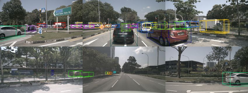
11Figure 4. Qualitative results generated with our approach and projected into the 360◦ images.
A.4. Runtime Analysis
We test the runtime of our algorithm on an Nvidia Ti-
tanXp GPU. The runtime of the different components per
frame is given in Table 4. Complete refers to a complete
iteration from generating the tracking graph to returning a
list of active tracks. A complete iteration consists of three
parts: First the graph datastructure is generated from the
detections and active tracks. Secondly, NMP is performed
and the nodes and edges are classified. Finally, tracks are
continued, terminated or initialized based on the classifica-
tion results during post-processing.
All numbers should be interpreted in the context of the
usual sampling rate of 10Hz for LIDAR scanners and the ef-
fective sampling rate of 2Hz that is used in the nuScenes [4]
dataset. With 12 fps for the complete pipeline, the method
can run at the sampling rate of a LIDAR and far above the
sampling rate of 2Hz used for tracking in this work.
Optimizing NMP and classification for a production
level implementation could yield some reduction in run-
Figure 5. Qualitative results generated with our approach projected
into the top-down view containing LIDAR points.
time. More importantly, graph generation and post-
processing is know to be slow in Python and an implementa-
tion in a more efficient programming language may improve
the runtime by multiple magnitudes. With around 70% of
For the proposed online-training, in the first stage, a net-
the runtime in these components, the real-time capability of
work is trained with data generated from the object detec-
the pipeline is further emphasized.
tions together with ground truth labels, the step we call
offline-training. This way the first set of tracks can be
formed, which all have corresponding ground truth tracks. Module Latency fps
In the second stage, the trained network is used to generate Complete 81.3 ms 12.3
NMP + classification 23.4 ms 42.7
track candidates, where some are close to the ground truth
Graph generation 24.9 ms 41.7
data, but some tracks also come from false positives and
Post-processing 32.9 ms 30.4
should not be matched by the algorithm. This set of tracks
cannot easily be represented with the data generated from Table 4. Inference time of our algorithm on a Nvidia Titan Xp in
detections and ground truth data alone, and thus, helps our the full online setting. All results are measured on the nuScenes[4]
method to perform better in the closed-loop-setting. validation set.
12A.5. Qualitative Results
Qualitative results achieved with our proposed tracker
are shown in Figures 4 and 5. The images show the 360◦
view as well as the rendered LIDAR detections of a typical
crowded scenario where our tracker outperforms previous
methods.
A.6. Failure Cases
During analyzing the qualitative results generated with
our tracker, following failure cases have been identified: (i)
Long frame gaps cause scenarios where the time a track
is kept active without observations is shorter than the ob-
served occlusion time. While extending this timeframe may
further reduce the number of ID-switches, it also increases
the number of false positives, harming the overall tracking
performance. (ii) Consistent false positive detections are a
general problem for any tracker following the tracking-by-
detection paradigm. While our tracker can easily handle
isolated false positives due to noise in the detector, cases
where e.g. physical structures or reflections are detected
cannot be recognized. (iii) Double objects are generated if
the same object is detected multiple times as different types.
This behavior can mostly be observed for trucks in our re-
sults and should be approached at the detector level e.g. with
non-maximum suppression[33].
It is important to note that all of these scenarios are
also failure cases for existing trackers, including the cur-
rent state-of-the-art CenterPoint[29], and are not introduced
by our pipeline. Furthermore, while the presented method
already reduces the number of such scenarios, further im-
proving the robustness is an interesting line of future work
in 3d detection and tracking.
13You can also read