LOGICAL ACTIVATION FUNCTIONS: EQUIVALENTS OF BOOLEAN OPERATORS - OpenReview
←
→
Page content transcription
If your browser does not render page correctly, please read the page content below
Under review as a conference paper at ICLR 2022

L OGICAL ACTIVATION F UNCTIONS : L OGIT- SPACE
EQUIVALENTS OF B OOLEAN O PERATORS

 Anonymous authors
 Paper under double-blind review

                                             A BSTRACT

         The choice of activation functions and their motivation is a long-standing issue
         within the neural network community. Neuronal representations within artificial
         neural networks are commonly understood as logits, representing the log-odds
         score of presence (versus absence) of features within the stimulus. In this work,
         we investigate the implications on activation functions of considering features to
         be logits. We derive operations equivalent to AND, OR, and XNOR for log-odds
         ratio representations of independent probabilities. Since these functions involve
         taking multiple exponents and logarithms, they are not well suited to be directly
         used within neural networks. Consequently, we construct efficient approximations
         named ANDAIL (the AND operator Approximate for Independent Logits), ORAIL ,
         and XNORAIL , which utilize only comparison and addition operations and can
         be deployed as activation functions in neural networks. Like MaxOut, ANDAIL
         and ORAIL are generalizations of ReLU to two-dimensions. We deploy these new
         activation functions, both in isolation and in conjunction, and demonstrate their
         effectiveness on a variety of tasks including image classification, transfer learning,
         abstract reasoning, and compositional zero-shot learning.

1    I NTRODUCTION

An activation function is a non-linearity which is interlaced between linear layers within an artificial
neural network. The non-linearity is essential in order for higher-order representations to form, since
otherwise the network would be degeneratively equivalent to a single linear layer.
Early artificial neural networks were inspired by biological neural networks, with the activation
function analogous to a neuron’s need to exceed a potentiation threshold in order to fire an action
potential. Biological neurons are have long been known to be more complex than this simple
abstraction, including features such as non-linearities in dendritic integration. Recent work has
demonstrated that a single biological neuron can compute the XOR of its inputs (Gidon et al., 2020),
a property long known to be lacking in artificial neurons (Minsky & Papert, 1969). This suggests that
gains in artificial neurons can be made by using activation functions which operate on more than one
input to the neuron at once.
The earliest artificial neural networks featured either logistic-sigmoid or tanh as their activation
function. These activation functions were motivated by the idea that each layer of the network is
building another layer of abstraction of the stimulus space from the last layer. Each neuron in a layer
identifies whether certain properties or features are present within the stimulus, and the pre-activation
(potentiation) value of the neuron indicates a score or logit for the presence of that feature. The
sigmoid function, σ(x) = 1/(1+e−x ), was hence a natural choice of activation function, since as with
logistic regression, this will convert the logits of features into probabilities.
There is some evidence that this interpretation has merit. Previous work has been done to identify
which features neurons are tuned to. Examples include LSTM neurons tracking quotation marks,
line length, and brackets (Karpathy et al., 2015); LSTM neurons tracking sentiment (Radford et al.,
2017); methods for projecting features back to the input space to view them (Olah et al., 2017); and
interpretable combinations of neural activities (Olah et al., 2020). Analogously, within biological
neural networks, neurons are tuned to respond more strongly to certain stimuli, and less strongly to

                                                   1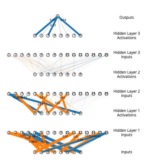
Under review as a conference paper at ICLR 2022

others. At high representation levels, concept cells respond predominantly to certain concepts, such
one’s grandmother, or Jennifer Aniston (Gross, 2002; Quian Quiroga et al., 2005).
Sigmoidal activation functions are no longer commonly used within machine learning between
layers of representations, though sigmoid is still widely used for gating operations which scale the
magnitude of other features in an attention-like manner. The primary disadvantage of the sigmoid
activation function is its vanishing gradient — as the potentiation rises, activity converges to a plateau,
and hence the gradient goes to zero. This prevents feedback information propagating back through
the network from the loss function to the early layers of the network, which consequently prevents it
from learning to complete the task.
The Rectified Linear Unit activation function (Fukushima, 1980; Jarrett et al., 2009; Nair & Hinton,
2010), ReLU(x) = max(0, x), does not have this problem, since in its non-zero regime it has a
gradient of 1. Another advantage of ReLU is it has very low computational demands. Since it is both
effective and efficient, it has proven to be a highly choice of popular activation function. The chief
drawback to ReLU is it has no sensitivity to changes across half of its input domain, and on average
passes no gradient back to its inputs. This can lead to neurons dying1 if their weights make them
never reach their activation threshold. If sigmoid is equivalent to converting our feature logits into
probabilities, then the ReLU activation function is equivalent to truncating our logits and denying any
evidence for the absence of a feature. We hypothesise that omitting negative evidence in this way is
undesirable and reduces the generalisation ability of ReLU-based networks.
Variants of ReLU have emerged, aiming to smooth out its transition between domains and provide
a gradient in its inactive regime. These include ELU (Clevert et al., 2016), CELU (Barron, 2017),
SELU (Klambauer et al., 2017), GELU (Hendrycks & Gimpel, 2020), SiLU (Elfwing et al., 2017;
Ramachandran et al., 2017), and Mish (Misra, 2019). However, all these activation functions still
bear the general shape of ReLU and truncate negative logits.
Fuzzy logic operators are generalizations of boolean logic operations to continuous variables, using
rules similar to applying logical operators in probability space. Previous work has explored networks
of fuzzy logic operations, including neural networks which use an activation functions that constitutes
a learnable interpolation between fuzzy logic operators (Godfrey & Gashler, 2017). In this work, we
introduce activation functions which are similar to fuzzy logic operators, but derived for working in
logit space instead of in probability space.
In this work we set out to develop activation functions based on the principle that neurons encode
logits — scores that represent the presence of features in the log-odds space. In Section 2 we derive
and define these functions in detail for different logical operators, and then consider their performance
on numerous task types including parity (Section 3.1), image classification (Sections 3.4 and 3.5),
transfer learning (Section 3.6), abstract reasoning (Appendix A.14), soft-rule guided classification
as exemplified by the Bach chorale dataset (Section 3.3), and compositional zero-shot learning (Ap-
pendix A.15). These tasks were selected to (1) survey the performance of the new activations on
existing benchmark tasks, and (2) evaluate their performance on tasks which we suspect in particular
may require logical reasoning and hence benefit from activation functions which apply these logical
operations to logits.

2       D ERIVATION

Manipulation of probabilities in logit-space is known to be more efficient for many calculations.
For instance, the log-odds form of Bayes’ Rule (Equation 9) states that the posterior logit equals
the prior logit plus the log of the likelihood ratio for the new evidence (the log of the Bayes
factor).Thus, working in logit-space allows us to perform Bayesian updates on many sources of
evidence simultaneously, merely by summing together the log-likelihood ratios for the evidence.
A weighted sum may be used if the amount of credence given to the sources differs — and this is
precisely the operation performed by a linear layer in a neural network.
When considering sets of probabilities, a natural choice of operation to perform is measuring the joint
probability of two events both occurring — the AND operation for probabilities. Suppose our input
space is x ∈ [0, 1]2 , and the goal is to output y > 0 if xi = 1 ∀ i, and y < 0 otherwise, using model
    1
        Though this problem is very rare when using BatchNorm to stabilise feature distributions.

                                                         2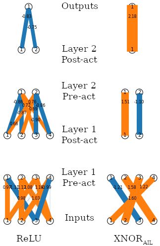
Under review as a conference paper at ICLR 2022

with a weight vector w and bias term b, such that y = wT x + b. This can be trivially solved with the
weight matrix w = [1, 1] and bias term b = −1.5. However, since this is only a linear separator, the
solution can not generalise to the case y > 0 iff xi > 0 ∀ i.
Similarly, let us consider how the OR function solved with a linear layer. Our goal is to output y > 0
if ∃ xi = 1, and y < 0 otherwise. The binary case can be trivially solved with the weight matrix
w = [1, 1] and bias term b = −0.5. The difference between this and the solution for AND is only an
offset to our bias term. In each case, if the input space is expanded beyond binary to R2 , the output
can be violated by changing only one of the arguments.

2.1   AND

Suppose we are given x and y as the logits for the presence (vs absence) of two events, X and Y .
These logits have equivalent probability values, which can be obtained using the sigmoid function,
σ(u) = (1 + e−u )−1 . Let us assume that the events X and Y are independent of each other. In this
case, the probability of both events occurring (the joint probability) is P(X, Y ) = P(X ∧ Y ) =
P(X) P(Y ) = σ(x) σ(y).
However, we wish to remain in logit-space, and must determine the logit of the joint probability,
logit(P(X, Y )). This is given by

                                                      p
           ANDIL := logit(P(X ∧ Y )x⊥  ⊥y ) = log          , where p = σ(x) σ(y),
                                                    1−p

                                                      σ(x) σ(y)
                                            = log                   ,                        (1)
                                                    1 − σ(x) σ(y)
which we coin as ANDIL , the AND operator for independent logits (IL). This 2d function is illustrated
as a contour plot (Figure 1, left). Across the plane, the order of magnitude of the output is the same
as at least one of the two inputs, scaling approximately linearly.
The approximately linear behaviour of the function is suitable for use as an activation function
(no vanishing gradient), however taking exponents and logs scales poorly from a computational
perspective. Hence, we developed a computationally efficient approximation as follows. Observe
that we can loosely approximate ANDIL with the minimum function (Figure 1, right panel). This is
equivalent to assuming the probability of both X and Y being true equals the probability of the least
likely of X and Y being true — a naı̈ve approximation which holds well in three quadrants of the
plane, but overestimates the probability when both X and Y are unlikely. In this quadrant, when both
X and Y are both unlikely, a better approximation for ANDIL is the sum of their logits.
We thus propose ANDAIL , a linear-approximate AND function for independent logits (AIL, i.e.
approximate IL).

                                           x + y,     x < 0, y < 0
                     ANDAIL (x, y) :=                                                   (2)
                                           min(x, y), otherwise
As shown in Figure 1 (left, middle), we observe that their output values and shape are very similar.

                     AND   IL                     ANDAIL                      min
                                                                                             +10
       4                                                                                     +8
                                                                                             +6
       2                                                                                     +4
                                                                                             +2
       0                                                                                     +0
                                                                                             −2
      −2                                                                                     −4
                                                                                             −6
      −4                                                                                     −8
                                                                                             −10
           −4   −2    0         2   4   −4   −2     0       2   4   −4   −2    0    2   4

Figure 1: Heatmap comparing the outputs for the exact logit-space probabilistic-and function for
independent logits, ANDIL (x, y); our constructed approximation, ANDAIL (x, y); and max(x, y).

                                                        3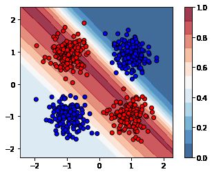
Under review as a conference paper at ICLR 2022

2.2   OR

Similarly, we can construct the logit-space OR function, for independent logits. For a pair of logits x
and y, the probability that either of the corresponding events is true is given by p = 1 − σ(−x) σ(−y).
This can be converted into a logit as

                                                           p
       ORIL (x, y) := logit(P(X ∨ Y )x⊥     ⊥y ) = log            , where p = 1 − σ(−x) σ(−y) (3)
                                                         1−p
which can be roughly approximated by the max function. This is equivalent to setting the probability
of either of event X or Y occurring to be equal to the probability of the most likely event. This
underestimates the upper-right quadrant (below), which we can approximate better as the sum of the
input logits, yielding
                                              x + y,      x > 0, y > 0
                          ORAIL (x, y) :=                                                       (4)
                                              max(x, y), otherwise

                   OR    IL                      ORAIL                       max
                                                                                                +10
       4                                                                                        +8
                                                                                                +6
       2                                                                                        +4
                                                                                                +2
       0                                                                                        +0
                                                                                                −2
      −2                                                                                        −4
                                                                                                −6
      −4                                                                                        −8
                                                                                                −10
           −4 −2     0        2    4     −4 −2     0       2   4   −4   −2    0    2   4

Figure 2: Comparison of the exact logit-space probabilistic-or function for independent logits,
ORIL (x, y); our constructed approximation, ORAIL (x, y); and max(x, y).

2.3   XNOR

We also consider the construction of a logit-space XNOR operator. This is the probability that X and
Y occur either together, or not at all, given by

                                                                        p
                                                    ¯
                     XNORIL (x, y) := logit(P(X ⊕Y )x⊥  ⊥y ) = log             ,                  (5)
                                                                     1−p
where p = σ(x) σ(y) + σ(−x) σ(−y). We can approximate this with
                                  XNORAIL (x, y) := sgn(xy) min(|x|, |y|),                            (6)
which focuses on the logit of the feature most likely to flip the expected parity (Figure 3).
We could use other approximations, such as the sign-preserving geometric mean,
                                                              p
                           signed geomean(x, y) := sgn(xy) |xy|,                                      (7)
but note that the gradient of this is divergent, both along x = 0 and along y = 0.

2.4   D ISCUSSION

By working via probabilities, and assuming inputs encode independent events, we have derived
logit-space equivalents of the boolean logic functions, AND, OR, and XNOR. Since these are
computationally demanding to compute repeatedly within a neural network, we have constructed
approximations of them: ANDAIL , ORAIL , and XNORAIL . Like ReLU, these involve only com-
parison, addition, and multiplication operations which are cheap to perform. In fact, ANDAIL and
ORAIL are a generalization of ReLU to an extra dimension, since ORAIL (x, y = 0) = max(x, 0).
The majority of activation functions are one-dimensional, f : R → R. In contrast to this, our proposed
activation functions are all two-dimensional, f : R2 → R. They must be applied to pairs of features

                                                       4
Under review as a conference paper at ICLR 2022

                   XNOR   IL                 XNORAIL                   signed_geomean
                                                                                               +10
       4                                                                                       +8
                                                                                               +6
       2                                                                                       +4
                                                                                               +2
       0                                                                                       +0
                                                                                               −2
      −2                                                                                       −4
                                                                                               −6
      −4                                                                                       −8
                                                                                               −10
           −4 −2     0         2   4   −4 −2     0       2   4    −4    −2   0    2     4

Figure 3: Comparison of the exact logit-space probabilistic-xnor function for independent logits,
XNORIL (x, y); our constructed approximation, XNORAIL (x, y); and signed geomean(x, y).

from the embedding space, and will reduce the dimensionality of the input space by a factor of 2. This
behaviour is the same as seen in MaxOut networks (Goodfellow et al., 2013) which use max as their
activation function, MaxOut(x, y; k) := max(x, y). Similar to MaxOut, our activation functions
could be generalised to higher dimensional inputs, f : Rk → R, by considering the behaviour of the
logit-space AND, OR, XNOR operations with regard to more inputs. For simplicity, we restrict this
work to consider only k = 2, but note these activation functions also generalize to higher dimensions.

2.5   E NSEMBLING

By using multiple logit-boolean activation functions simultaneously alongside each other, we permit
the network multiple options of how to relate features together. When combining the activation
functions, we considered two strategies.
In the partition (p) strategy, we split the nc dimensional pre-activation embedding equally into m
partitions, apply different activation functions on each partition, and concatenate the results together.
Using AIL activation functions under this strategy, the output dimension will always be half that of
the input, as it is for each AIL activation function individually.
In the duplication (d) strategy, we apply m different activation functions in parallel to the same nc
elements. The output is consequently larger, with dimension m nc . If desired, we can counteract the
2 → 1 reduction of AIL activation functions by using two of them together under this strategy.
Utilising ANDAIL , ORAIL and XNORAIL simultaneously allows our networks to access logit-space
equivalent of 12 of the 16 boolean logical operations with only a single sign inversion (in either one
of the inputs or the output). Including the bias term and skip connections, the network has easy access
to logit-space equivalents of all 16 boolean logical operations.

3     E XPERIMENTS
We evaluated the performance of our AIL activation functions, both individually and together in an
ensemble, on a range of benchmarking tasks. Since ANDAIL and ORAIL are equivalent when the
sign of operands and outputs can be freely chosen, we evaluate only on ORAIL and not both.
We compared the AIL activation functions against three primary baselines: (1) ReLU, (2)
max(x, y) = MaxOut([x, y]; k = 2), and (3) the concatenation of max(x, y) and min(x, y), denoted
{Max, Min (d)}. The {Max, Min (d)} ensemble is equivalent to GroupSort with a group size of 2
(Anil et al., 2019; Chernodub & Nowicki, 2017), sometimes referred to as the MaxMin operator, and
is comparable to the concatenation of ORAIL and ANDAIL under our duplication strategy.

3.1   PARITY

In a simple initial experiment, we constructed a synthetic dataset whose labels could be derived
directly using the logical operation XNOR. Each sample in this dataset consisted of four input logit
values, with a label that was derived by converting each logit to probability space, rounding to the

                                                     5
Under review as a conference paper at ICLR 2022
nearest integer, and taking the parity over this set of binary digits (i.e. true when we have an even
number of activated bits, false otherwise).
A very small MLP model with two hidden lay-
ers (the first with four neurons, the second
with two neurons) should be capable of per-
fect classification accuracy on this dataset with
a sparse weight matrix by learning to extract
pairwise binary relationships between inputs us-
ing XNORAIL . We trained such an MLP, for
100 epochs using Adam, one-cycle learning rate
schedule, max LR 0.01, weight decay 1 × 10⁻⁴ .
The two-layer MLP using the XNORAIL acti-
vation learned a sparse weight matrix able to
perfectly classify any input combination, shown
in Figure 4. In comparison, an identical network
setup using ReLU was only able to produce 60%
classification accuracy. Though this accuracy
could be improved by increasing the MLP width
or depth, the weight matrix was still not sparse.
This experiment provides an example situation
where XNORAIL is utilized by a network to
directly extract information about the relation-
ships between network inputs. For additional
results, see Appendix A.7.
3.2 MLP ON C OVERTYPE
Figure 4: Visualisation of weight matrices learnt
We trained small one, two, and three-layer MLP by two-layer MLPs on a binary classification task,
models on the Covertype dataset (UCI Machine where the target output is the parity of the inputs.
Learning Repository, 1998; Blackard & Dean, Widths of lines indicate weight magnitudes (or-
1998) from the UCI Machine Learning Repos- ange: +ve values, blue: -ve). Network with ReLU:
itory. The Covertype dataset is a classification 60% accuracy. Network with XNORAIL : 100%
task consisting of 581 012 samples of forest cov- accuracy.
erage across 7 classes. Each sample has 54 at-
tributes. We used a fixed random 80:20 train:test
split; for training details and accuracy vs model
size, see Appendix A.8.
For each activation function, we varied the number of hidden units per layer to investigate how
the activation functions affected the performance of the networks as its capacity changed. We did
not use weight decay or data augmentation for this experiment, and so the network exhibits clear
overfitting with larger architectures. As shown in Figure 16, Appendix A.8, XNORAIL performs
significantly best on Covertype (p < 10−5 ) for MLP with 2 or 3 layers, followed by networks which
include XNORAIL alongside with other activations, and signed geomean. The duplication strategy
outperforms partition.
3.3 MLP ON BACH C HORALES AND L OGIT I NDEPENDENCE
The Bach Chorale dataset (Boulanger-Lewandowski et al., 2012) consists of 382 chorales composed
by JS Bach, each ∼12 measures long, totalling approximately 83,000 notes. Represented as discrete
sequences of tokens, it has served as a benchmark for music processing for decades, from heuristic
methods to HMMs, RNNs, and CNNs (Mozer, 1990; Hild et al., 1992; Allan & Williams, 2005;
Liang, 2016; Hadjeres et al., 2017; Huang et al., 2019). The chorales are comprised of 4 voices
(melodic lines) whose behaviour is guided by soft musical rules that depend on the prior movement of
that voice as well as the movement of the other voices. An example of one such rule is that two voices
a fifth apart ought not to move in parallel with one another. The task we choose here is to determine
whether a given short four-part musical excerpt is taken from a Bach chorale or not. During training,
we stochastically corrupt chorale excerpts to provide negative examples (see Appendix A.9). We
6Under review as a conference paper at ICLR 2022
trained 2-layer MLP discriminators with a single sigmoid output and exchanged all other activation
functions (summarized in Figure 17). We found that {OR, AND, XNORAIL (d)} performed best,
but that overall the results were comparable (p < 0.1 between best and worst, Student’s t-test between
10 random initialisations).
Additionally, we investigated the independence between logits in the trained pre-activation embed-
dings. We would expect that an MLP which is optimally engaging its neurons would maintain
independence between features in order to maximize information. To capture the existence of correla-
tions, we took the cosine similarity between rows of the weight matrix. Since the inputs to all features
in a given layer are the same, this is equivalent to measuring the similarity between corresponding
pair of pre-activation features. We performed two experiments. In the first, we measured correlations
between all pairwise combinations, and in the second we took correlations between only adjacent
pre-activations that would be paired for the logical activation functions. For these experiments we
used 2 hidden layers and a width that showed maximal performance for each activation function. The
results are shown in Appendix A.10.
3.4 CNN AND MLP ON MNIST
MNIST , MLP (2 hidden layers) MNIST, CNN (6 layer)
98.8
99.6
98.7
98.6 99.5
Test accuracy (%)
Test accuracy (%)
ReLU
98.5 SiLU
Max
98.4 Max, Min (d) 99.4
signed_geomean
98.3 XNOR AIL
ORAIL
99.3
98.2 OR, AND (d) AIL
OR, XNOR (p) AIL
98.1 OR, XNOR (d) AIL
OR, AND, XNOR (p) 99.2
98.0
AIL
OR, AND, XNOR (d) AIL
105 106 107 104 105 106 107
Number of parameters Number of parameters
Figure 5: We trained CNN on MNIST, MLP on flattened-MNIST, using Adam (1-cycle, 10 ep),
hyperparams determined by random search. Mean (bars: std dev) of n = 40 weight inits.
We trained 2-layer MLP and 6-layer CNN models on MNIST with Adam (Kingma & Ba, 2017),
1-cycle schedule (Smith & Topin, 2017; Smith, 2018), and using hyperparameters tuned through a
random search against a validation set comprised of the last 10k images of the training partition.
The MLP used two hidden layers, the widths of which were varied together to evaluate the perfor-
mance for a range of model sizes. The CNN used six layers of 3x3 convolution layers, with 2x2 max
pooling (stride 2) after every other conv layer. The output was flattened and followed by three MLP
layers. The widths of the layers were scaled up approximately linearly to explore a range of model
sizes (see Appendix A.11 for more details).
For the MLP, XNORAIL performed best along with signed geomean (p < 0.1), ahead of all
other activations (p < 0.01; Figure 5 left panel). With the CNN, five activation configurations
({OR, AND, XNORAIL (p)}, {OR, XNORAIL (d/p)}, Max, and SiLU) performed best (p < 0.05;
Figure 5, right panel). Additionally, we note that CNNs which used ORAIL or Max (alone or in an
ensemble) maintained high performance with an order of magnitude fewer parameters (3 × 10⁴ ) than
networks which did not (3 × 10⁵ params).
3.5 R ES N ET 50 ON CIFAR-10/100
We explored the impact of our AIL activation functions on the performance of deep networks by
deploying them within a pre-activation ResNet50 model (He et al., 2015; 2016). We exchanged all
ReLU activation functions in the network to a candidate activation function while maintaining the
size of pass-through embedding. We experimented with changing the width of the network, scaling
up the embedding space and all hidden layers by a common factor. The network was trained on
7Under review as a conference paper at ICLR 2022
CIFAR-10/-100 for 100 epochs using Adam (Kingma & Ba, 2017), 1-cycle (Smith, 2018; Smith
& Topin, 2017). Hyperparameters were optimized through a random search against a validation
partition of CIFAR-100 for a fixed width factor w = 2 only. The same hyperparameters were reused
for experiments of changing width, and for CIFAR-10. We used width factors of 0.5, 1, 2, and 4 for
1 → 1 activation functions (ReLU, etc), widths of 0.75, 1.5, 3, and 6 for 2 → 1 activation functions
(Max, etc), and widths of 0.4, 0.75, 1.5, and 3 for {ORAIL , ANDAIL , XNORAIL (d)}.
CIFAR-10, ResNet50 CIFAR-100, ResNet50
96.0
79
95.5
78
95.0
Test accuracy (%)
Test accuracy (%)
ReLU 77
PReLU
94.5 SiLU 76
Max
94.0 Max, Min (d) 75
ORAIL
OR, AND (d) 74
93.5 OR, XNOR (d)
OR, AND, XNOR (d) 73
OR, XNOR (p)
93.0 OR, AND, XNOR (p)
72
107 108 107 108
Number of parameters Number of parameters
Figure 6: ResNet50 on CIFAR-10/100, varying the activation function. The same activation function
(or ensemble) was used through the network. The width was varied to explore a range of network
sizes (see text). Trained for 100 ep. with Adam, using hyperparams determined by random search on
CIFAR-100, w = 2, only.
For both CIFAR-10 and 100, we find that SiLU, ORAIL , and Max outperform ReLU across a
wide range of width values, as shown in Figure 6. These three activation functions hold up their
performance best as the number of parameters is reduced. Note that SiLU was previously discovered
as an optimal activation function for deep residual image models (Ramachandran et al., 2017), and so
it is expected to perform highly in this setting. Meanwhile, other AIL activation functions perform
similarly to ReLU when the width is thin, and slightly worse than ReLU when the width is wide.
When used on its own and not part of an ensemble, the XNORAIL activation function performed
very poorly (off the bottom of the chart), indicating it is not well suited for this task.
3.6 T RANSFER LEARNING
We considered the task of transfer learning on several image classification datasets. We used
a ResNet18 model (He et al., 2015) pretrained on ImageNet-1k. The weights were frozen (not
fine-tuned) and used to generate embeddings of samples from other image datasets. We trained a two-
layer MLP to classify the images from these embeddings, using various activation functions. For a
comprehensive set of baselines, we compared against every activation function built into PyTorch 1.10.
To make the number of parameters similar, we used a width of 512 for activation functions with
1 → 1 mapping (e.g. ReLU), a width of 650 for activation functions with a 2 → 1 mapping (e.g. Max,
ORAIL ), and a width of 438 for {OR, AND, XNORAIL (d)}. See Appendix A.13 for more details.
Our results are shown in Table 1. We found that all our activation functions outperformed ReLU
on every transfer task. In particular, our three activation ensembles using the duplication strategy
performed very highly across all 7 transfer learning tasks — overall, {OR, AND, XNORAIL (d)}
appears to perform best (top for 3 datasets, second on 3), followed by {OR, ANDAIL (d)}. Our
activation functions were beaten on Caltech101, Oxford Flowers, and Stanford Cars, and only
by PReLU. For these three datasets, a linear readout outperformed an MLP with ReLU, and on
Caltech101 the linear layer performed best. This suggests that PReLU excels only on particularly
simple tasks. For further discussion, see Appendix A.13.
3.7 A DDITIONAL RESULTS
For results on abstract reasoning and compositional zero-shot learning, please see Appendix A.14
and Appendix A.15, respectively.
8Under review as a conference paper at ICLR 2022
Table 1: Transfer learning from a frozen ResNet-18 architecture pretrained on ImageNet-1k to other
computer vision datasets. An MLP head with two layers of pre-activation width of either 438, 512, or
650 (depending on activation function, to keep the number of params approximately constant) was
trained, without re-training the pretrained base model. Trained with SGD, cosine annealed LR 0.01,
for 25 epochs. Mean (standard error) of n = 5 random initializations of the MLP (same pretrained
network). Bold: best. Underlined: second best. Italic: no significant difference from best (two-sided
Student’s t-test, p > 0.05). Background: linear color scale from ReLU baseline (white) to best (black).
Test Accuracy (%)
Activation function Caltech101 CIFAR10 CIFAR100 Flowers Cars STL-10 SVHN
Linear layer only 88.35±0.15 78.56±0.09 57.39±0.09 92.32±0.20 33.51±0.06 94.68±0.02 45.42±0.06
ReLU 86.58±0.17 81.63±0.05 58.04±0.11 90.71±0.26 30.97±0.26 94.62±0.06 51.39±0.06
LeakyReLU 86.60±0.13 81.67±0.11 58.01±0.09 90.73±0.32 31.09±0.24 94.61±0.05 51.40±0.05
PReLU 87.83±0.21 81.03±0.13 58.90±0.18 93.17±0.19 39.84±0.18 94.54±0.05 51.42±0.09
Softplus 86.16±0.18 79.13±0.08 56.58±0.07 89.39±0.29 21.23±0.13 94.63±0.03 47.44±0.06
ELU 87.18±0.09 80.44±0.08 58.08±0.10 91.71±0.14 34.70±0.06 94.55±0.05 50.07±0.07
CELU 87.18±0.09 80.44±0.08 58.08±0.10 91.71±0.14 34.70±0.06 94.55±0.05 50.07±0.07
SELU 87.74±0.09 79.93±0.13 58.24±0.06 92.27±0.13 37.51±0.17 94.53±0.07 49.38±0.06
GELU 87.10±0.15 81.39±0.09 58.51±0.13 91.51±0.15 33.43±0.15 94.62±0.06 51.56±0.08
SiLU 86.91±0.11 80.53±0.11 58.14±0.12 91.37±0.18 32.15±0.17 94.59±0.05 50.69±0.09
Hardswish 87.12±0.12 80.10±0.10 58.25±0.10 91.56±0.25 33.17±0.23 94.62±0.05 50.09±0.09
Mish 87.11±0.12 81.09±0.11 58.37±0.10 91.61±0.15 33.75±0.14 94.61±0.05 51.29±0.08
Softsign 81.47±0.18 80.03±0.09 54.84±0.09 82.34±0.22 17.33±0.10 94.70±0.03 49.48±0.07
Tanh 87.48±0.06 80.56±0.07 57.35±0.08 90.32±0.20 29.51±0.12 94.63±0.07 50.15±0.08
GLU 86.71±0.31 79.19±0.07 57.64±0.10 90.34±0.19 27.04±0.12 94.57±0.03 48.28±0.17
Max 86.96±0.20 81.76±0.14 58.60±0.12 90.98±0.18 33.37±0.15 94.70±0.06 51.36±0.12
Max, Min (d) 87.23±0.13 82.31±0.10 59.05±0.10 91.68±0.18 34.91±0.12 94.64±0.04 51.72±0.04
XNORAIL 86.97±0.18 81.83±0.06 58.46±0.10 90.93±0.15 32.56±0.10 94.71±0.06 51.54±0.05
ORAIL 87.45±0.14 81.88±0.07 59.10±0.09 92.00±0.15 36.01±0.12 94.69±0.04 51.52±0.07
OR, ANDAIL (d) 87.43±0.11 82.38±0.06 59.90±0.08 92.07±0.18 37.16±0.15 94.55±0.05 52.11±0.09
OR, XNORAIL (p) 87.42±0.12 81.92±0.07 59.09±0.10 91.93±0.12 35.99±0.17 94.68±0.03 51.43±0.08
OR, XNORAIL (d) 87.09±0.21 82.20±0.04 59.44±0.07 91.90±0.10 36.88±0.10 94.69±0.06 52.02±0.16
OR, AND, XNORAIL (p) 87.43±0.14 81.78±0.06 59.27±0.13 91.98±0.29 35.90±0.09 94.66±0.03 51.47±0.13
OR, AND, XNORAIL (d) 87.49±0.11 82.50±0.08 59.83±0.12 92.37±0.08 37.60±0.20 94.72±0.02 52.23±0.14
4 D ISCUSSION
In this work we motivated and introduced novel activation functions analogous to boolean operators
in logit-space. We designed the AIL functions, fast approximates to the true logit-space functions
equivalent to manipulating the corresponding probabilities, and demonstrated their effectiveness on a
wide range of tasks.
Although our activation functions assume independence (which is generally approximately true for the
pre-activation features learnt with 1d activation functions), we found the network learnt to induce anti-
correlations between features which were paired together by our activation functions (Appendix A.10).
This suggests that the assumption of independence is not essential to the performance of our proposed
activation functions.
We found that the XNORAIL activation function was highly effective in the setting of shallow net-
works. Meanwhile, the ORAIL activation function was highly effective for representation learning in
the setting of a deep ResNet architecture trained on images. In scenarios which involve manipulating
high-level features extracted by an embedding network, we find that using an ensemble of AIL
activation functions together works best, and that the duplication ensembling strategy outperforms
partitioning. In this work we have restricted ourselves to only considering using a single activation
function (or ensemble) throughout the network, however our results together indicate that stronger re-
sults may be found by using ORAIL for feature extraction and an ensemble of {OR, AND, XNORAIL
(d)} for later higher-order reasoning layers within the network.
The idea we propose is nascent and there is a great deal of scope for exploring other forms of
activation functions that combine multiple pre-activation features by utilizing “higher-order activation
functions”.
9Under review as a conference paper at ICLR 2022
R EPRODUCIBILITY S TATEMENT
We have shared code to run all experiments considered in this paper with the reviewers via an anony-
mous download URL. The code base contains detailed instructions on how to setup each experiment,
including downloading the datasets and installing environments with pinned dependencies. It should
be possible to reproduce all our experimental results with this code. For the final version of the paper,
we will make the code publicly available on an online repository and share a link to it within the
paper.
R EFERENCES
Moray Allan and Christopher Williams. Harmonising chorales by probabilistic inference. In L. Saul,
Y. Weiss, and L. Bottou (eds.), Advances in Neural Information Processing Systems, volume 17.
MIT Press, 2005.
Cem Anil, James Lucas, and Roger Grosse. Sorting out lipschitz function approximation, 2019.
David G. T. Barrett, Felix Hill, Adam Santoro, Ari S. Morcos, and Timothy Lillicrap. Measuring
abstract reasoning in neural networks, 2018.
Jonathan T. Barron. Continuously differentiable exponential linear units, 2017.
Yaniv Benny, Niv Pekar, and Lior Wolf. Scale-localized abstract reasoning, 2021.
Jock A. Blackard. Comparison of Neural Networks and Discriminant Analysis in Predicting Forest
Cover Types. PhD thesis, Colorado State University, USA, 1998. AAI9921979.
Jock A Blackard and Denis J Dean. Comparative accuracies of neural networks and discriminant
analysis in predicting forest cover types from cartographic variables. In Second Southern Forestry
GIS Conference, pp. 189–199, 1998.
Nicolas Boulanger-Lewandowski, Yoshua Bengio, and Pascal Vincent. Modeling temporal dependen-
cies in high-dimensional sequences: Application to polyphonic music generation and transcription,
2012.
Artem Chernodub and Dimitri Nowicki. Norm-preserving orthogonal permutation linear unit activa-
tion functions (oplu), 2017.
Djork-Arné Clevert, Thomas Unterthiner, and Sepp Hochreiter. Fast and accurate deep network
learning by exponential linear units (elus), 2016.
Adam Coates, Andrew Ng, and Honglak Lee. An analysis of single-layer networks in unsupervised
feature learning. In Proceedings of the fourteenth international conference on artificial intelligence
and statistics, pp. 215–223. JMLR Workshop and Conference Proceedings, 2011.
Ekin Dogus Cubuk, Barret Zoph, Dandelion Mané, Vijay Vasudevan, and Quoc V. Le. Autoaugment:
Learning augmentation policies from data. CoRR, abs/1805.09501, 2018. URL http://arxiv.
org/abs/1805.09501.
Stefan Elfwing, Eiji Uchibe, and Kenji Doya. Sigmoid-weighted linear units for neural network
function approximation in reinforcement learning, 2017.
Li Fei-Fei, Rob Fergus, and Pietro Perona. One-shot learning of object categories. IEEE transactions
on pattern analysis and machine intelligence, 28(4):594–611, 2006.
François Fleuret, Ting Li, Charles Dubout, Emma K. Wampler, Steven Yantis, and Donald Ge-
man. Comparing machines and humans on a visual categorization test. Proceedings of
the National Academy of Sciences, 108(43):17621–17625, 2011. ISSN 0027-8424. doi:
10.1073/pnas.1109168108. URL https://www.pnas.org/content/108/43/17621.
Kunihiko Fukushima. Neocognitron: A self-organizing neural network model for a mechanism of
pattern recognition unaffected by shift in position. Biological Cybernetics, 36(4):193–202, Apr
1980. ISSN 1432-0770. doi: 10.1007/BF00344251. URL https://doi.org/10.1007/
BF00344251.
10Under review as a conference paper at ICLR 2022
Albert Gidon, Timothy Adam Zolnik, Pawel Fidzinski, Felix Bolduan, Athanasia Papoutsi, Panayiota
Poirazi, Martin Holtkamp, Imre Vida, and Matthew Evan Larkum. Dendritic action poten-
tials and computation in human layer 2/3 cortical neurons. Science, 367(6473):83–87, 2020.
doi: 10.1126/science.aax6239. URL https://www.science.org/doi/abs/10.1126/
science.aax6239.
Luke B. Godfrey and Michael S. Gashler. A parameterized activation function for learning fuzzy
logic operations in deep neural networks. CoRR, abs/1708.08557, 2017. URL http://arxiv.
org/abs/1708.08557.
Ian Goodfellow, David Warde-Farley, Mehdi Mirza, Aaron Courville, and Yoshua Bengio. Maxout
networks. In Sanjoy Dasgupta and David McAllester (eds.), Proceedings of the 30th International
Conference on Machine Learning, volume 28 of Proceedings of Machine Learning Research, pp.
1319–1327, Atlanta, Georgia, USA, 17–19 Jun 2013. PMLR. URL https://proceedings.
mlr.press/v28/goodfellow13.html.
Charles G. Gross. Genealogy of the “grandmother cell”. The Neuroscientist, 8(5):512–518, 2002.
doi: 10.1177/107385802237175. URL https://doi.org/10.1177/107385802237175.
PMID: 12374433.
Gaëtan Hadjeres, François Pachet, and Frank Nielsen. Deepbach: a steerable model for bach chorales
generation, 2017.
Kaiming He, Xiangyu Zhang, Shaoqing Ren, and Jian Sun. Deep residual learning for image
recognition. CoRR, abs/1512.03385, 2015. URL http://arxiv.org/abs/1512.03385.
Kaiming He, Xiangyu Zhang, Shaoqing Ren, and Jian Sun. Identity mappings in deep residual
networks, 2016.
Dan Hendrycks and Kevin Gimpel. Gaussian error linear units (GELUs), 2020.
Hermann Hild, Johannes Feulner, and Wolfram Menzel. Harmonet: A neural net for harmonizing
chorales in the style of JS Bach. In Advances in neural information processing systems, pp.
267–274, 1992.
Sheng Hu, Yuqing Ma, Xianglong Liu, Yanlu Wei, and Shihao Bai. Stratified rule-aware network for
abstract visual reasoning, 2020.
Cheng-Zhi Anna Huang, Tim Cooijmans, Adam Roberts, Aaron Courville, and Douglas Eck. Coun-
terpoint by convolution, 2019.
Phillip Isola, Joseph J Lim, and Edward H Adelson. Discovering states and transformations in image
collections. In Proceedings of the IEEE conference on computer vision and pattern recognition,
pp. 1383–1391, 2015.
Kevin Jarrett, Koray Kavukcuoglu, Marc’Aurelio Ranzato, and Yann LeCun. What is the best
multi-stage architecture for object recognition? In 2009 IEEE 12th International Conference on
Computer Vision, pp. 2146–2153, 2009. doi: 10.1109/ICCV.2009.5459469.
Justin Johnson, Bharath Hariharan, Laurens van der Maaten, Li Fei-Fei, C. Lawrence Zitnick, and
Ross Girshick. Clevr: A diagnostic dataset for compositional language and elementary visual
reasoning. In Proceedings of the IEEE Conference on Computer Vision and Pattern Recognition
(CVPR), July 2017.
H M Dipu Kabir, Moloud Abdar, Seyed Mohammad Jafar Jalali, Abbas Khosravi, Amir F Atiya,
Saeid Nahavandi, and Dipti Srinivasan. Spinalnet: Deep neural network with gradual input, 2020.
Daniel Kahneman. Thinking, fast and slow. Thinking, fast and slow. Farrar, Straus and Giroux, New
York, NY, US, 2011. ISBN 0-374-27563-7 (Hardcover); 1-4299-6935-0 (PDF); 978-0-374-27563-1
(Hardcover); 978-1-4299-6935-2 (PDF).
Andrej Karpathy, Justin Johnson, and Li Fei-Fei. Visualizing and understanding recurrent networks,
2015.
11Under review as a conference paper at ICLR 2022
Diederik P. Kingma and Jimmy Ba. Adam: A method for stochastic optimization, 2017.
Günter Klambauer, Thomas Unterthiner, Andreas Mayr, and Sepp Hochreiter. Self-normalizing neural
networks. In Proceedings of the 31st international conference on neural information processing
systems, pp. 972–981, 2017.
Jonathan Krause, Michael Stark, Jia Deng, and Li Fei-Fei. 3d object representations for fine-grained
categorization. In 4th International IEEE Workshop on 3D Representation and Recognition
(3dRR-13), Sydney, Australia, 2013.
Alex Krizhevsky. Learning multiple layers of features from tiny images. Technical report, University
of Toronto, 2009.
Yann LeCun, Léon Bottou, Yoshua Bengio, and Patrick Haffner. Gradient-based learning applied to
document recognition. Proceedings of the IEEE, 86(11):2278–2324, 1998.
Feynman Liang. Bachbot: Automatic composition in the style of Bach chorales. University of
Cambridge, 8:19–48, 2016.
Marvin Minsky and Seymour Papert. Perceptrons. Perceptrons. M.I.T. Press, Oxford, England, 1969.
Diganta Misra. Mish: A self regularized non-monotonic neural activation function, 2019.
Michael C Mozer. Connectionist music composition based on melodic, stylistic, and psychophysical
constraints. University of Colorado, Boulder, Department of Computer Science, 1990.
Vinod Nair and Geoffrey Hinton. Rectified linear units improve restricted boltzmann machines.
volume 27, pp. 807–814, 06 2010.
Yuval Netzer, Tao Wang, Adam Coates, Alessandro Bissacco, Bo Wu, and Andrew Y Ng. Reading
digits in natural images with unsupervised feature learning. NIPS Workshop on Deep Learning
and Unsupervised Feature Learning, 2011.
Maria-Elena Nilsback and Andrew Zisserman. Automated flower classification over a large number
of classes. In 2008 Sixth Indian Conference on Computer Vision, Graphics & Image Processing,
pp. 722–729. IEEE, 2008.
Chris Olah, Alexander Mordvintsev, and Ludwig Schubert. Feature visualization. Distill, 2017. doi:
10.23915/distill.00007. https://distill.pub/2017/feature-visualization.
Chris Olah, Nick Cammarata, Ludwig Schubert, Gabriel Goh, Michael Petrov, and Shan Carter.
Zoom in: An introduction to circuits. Distill, 2020. doi: 10.23915/distill.00024.001.
Senthil Purushwalkam, Maximilian Nickel, Abhinav Gupta, and Marc’Aurelio Ranzato. Task-driven
modular networks for zero-shot compositional learning, 2019.
R Quian Quiroga, L Reddy, G Kreiman, C Koch, and I Fried. Invariant visual representation by single
neurons in the human brain. Nature, 435:1102–1107, 2005. doi: 10.1038/nature03687.
Alec Radford, Rafal Jozefowicz, and Ilya Sutskever. Learning to generate reviews and discovering
sentiment, 2017.
Prajit Ramachandran, Barret Zoph, and Quoc V. Le. Searching for activation functions, 2017.
John C Raven and JH Court. Raven’s progressive matrices. Western Psychological Services Los
Angeles, CA, 1938.
Jason Rennie, Lawrence Shih, Jaime Teevan, and David Karger. Tackling the poor assumptions of
naive bayes text classifiers. Proceedings of the Twentieth International Conference on Machine
Learning, 41, 07 2003.
Leslie N. Smith. A disciplined approach to neural network hyper-parameters: Part 1 - learning
rate, batch size, momentum, and weight decay. CoRR, abs/1803.09820, 2018. URL http:
//arxiv.org/abs/1803.09820.
12Under review as a conference paper at ICLR 2022
Leslie N. Smith and Nicholay Topin. Super-convergence: Very fast training of residual networks
using large learning rates. CoRR, abs/1708.07120, 2017. URL http://arxiv.org/abs/
1708.07120.
UCI Machine Learning Repository. Covertype data set, Aug 1998. URL https://archive.
ics.uci.edu/ml/datasets/Covertype.
Chi Zhang, Feng Gao, Baoxiong Jia, Yixin Zhu, and Song-Chun Zhu. RAVEN: A dataset for
relational and analogical visual reasoning. In Proceedings of the IEEE Conference on Computer
Vision and Pattern Recognition (CVPR), 2019.
13Under review as a conference paper at ICLR 2022
A A PPENDIX
A.1 L INEAR R E LU EXAMPLES
In Figure 7, we show a representation of what a 2-d linear layer followed by the ReLU activation
function looks like. The output is the same up to rotation.
Figure 7: ReLU unit, and ReLU units followed by a linear layer to try to approximate ORIL , leaving
a dead space where the negative logits should be.
If we apply a second linear layer on top of the outputs of the first two units, we can try to approximate
the logit AND or OR function. However, the solution using ReLU leaves a quadrant of the output
space hollowed out as zero due to its behaviour at truncating away information.
A.2 S OLVING XOR
A long-standing criticism of artificial neural networks is their inability to solve XOR with a single
layer (Minsky & Papert, 1969). Of course, adding a single hidden layer allows a network using
ReLU to solve XOR. However, the way that it solves the problem is to join two of the disconnected
regions together in a stripe (see Figure 8). Meanwhile, our XNORAIL is trivial able to solve the XOR
problem without any hidden layers. For comparison here, we include one hidden layer with 2 units for
each network. Including a layer before the activation function makes the task harder for XNORAIL ,
which must learn how to project the input space in order to compute the desired separation. Also,
including the linear layer allows the network to generalise to rotations and offset versions of the task.
14Under review as a conference paper at ICLR 2022
(a) ReLU (b) XNORAIL
Figure 8: Solving XOR with a single hidden layer of 2 units, using either ReLU or XNORAIL
activation. Circles indicate negative (blue) and positive (red) training samples. The heatmaps indicate
the output probabilities of the two networks.
A.3 L INEAR LAYERS AND BAYES ’ RULE IN LOG - ODDS FORM
Bayes’ Theorem or Bayes’ Rule is given by
P(X|H) P(H)
P(H|X) = . (8)
P(X)
In this case, we update the probability of our hypothesis, H, based on the event of the observation of
a new piece of evidence, X. Our prior belief for the hypothesis is P(H), and posterior is P(H|X).
To update our belief from the prior and yield the posterior, we multiply by the Bayes factor for the
evidence which is given by P(X|H)/P(X).
Converting the probabilities into log-odds ratios (logits) yields the following representation of Bayes’
Rule.
P(H|X) P(H) P(X|H)
log = log + log (9)
P(H C |X) P(H C ) P(X|H C )
Here, H C is the complement to H (the event that the hypothesis is false), and P(H C ) = 1 −
P(H). Our prior log-odds ratio is log ((P(H)/P(H C )), and our posterior after updating based on
the observation of new evidence X is log (P(H|X)/P(H C |X)). To update our belief from the prior
and yield the posterior, we add the log-odds Bayes factor for the evidence which is given by
log (P(X|H)/P(X|H C )).
In log-odds space, a series of updates with multiple pieces of independent evidence can be performed
at once with a summation operation.
X
P(H|x) P(H) P(Xi |H)
log = log + log . (10)
P(H C |x) P(H C ) i
P(Xi |H C )
This is operation can be represented by the linear layer in an artificial neural network, zk = bk +wkT x.
Here, the bias term bk = log ((P(H)/P(H C )) is the prior for hypothesis (the presence of the feature
represented by the k-th neuron), and the series of weighted inputs from the previous layer, wki xi
provide evidential updates. This is also equivalent to the operation of a multinomial naı̈ve Bayes
classifier, expressed in log-space, if we choose wki = log pki (Rennie et al., 2003).
A.4 D IFFERENCE BETWEEN AIL AND IL FUNCTIONS
Here, we measure and show the difference between the true logit-space operations and our AIL
approximations, shown in Figure 9, Figure 10, and Figure 11.
In each case, we observe that the magnitude of the difference is never more than 1, which occurs
along the boundary lines in AIL. Since the magnitude of the three functions increase as we move
away from the origin, the relative difference decreases in magnitude as the size of x and y increase.
15Under review as a conference paper at ICLR 2022
Figure 9: Heatmaps showing ANDIL , ANDAIL , their difference, and their relative difference.
Figure 10: Heatmaps showing ORIL , ORAIL , their difference, and their relative difference.
16Under review as a conference paper at ICLR 2022
Figure 11: Heatmaps showing XNORIL , XNORAIL , their difference, and their relative difference.
17Under review as a conference paper at ICLR 2022
A.5 G RADIENT OF AIL AND IL FUNCTIONS
We show the gradient of each of the logit-space boolean operators and their AIL approximates in
Figure 12, Figure 13, and Figure 14. By the symmetry of each of the functions, the derivative with
respect to y is a reflected copy of the gradient with respect to x.
We find that the gradient of each AIL function closely matches that of the exact form. Whilst there
are “dead” regions where the gradient is zero, this only occurs for one of the derivatives at a time
(there is always a gradient with respect to at least one of x and y).
Figure 12: Heatmaps showing the gradient with respect to x and y of ANDIL and ANDAIL .
18Under review as a conference paper at ICLR 2022
Figure 13: Heatmaps showing the gradient with respect to x and y of ORIL or ORAIL .
Figure 14: Heatmaps showing the gradient with respect to x and y of XNORIL xnor XNORAIL .
A.6 DATASET SUMMARY
The datasets used in this work are summarised in Table 2.
We used the same splits for Caltech101 as used in Kabir et al. (2020).
19Under review as a conference paper at ICLR 2022
Table 2: Dataset summaries.
№ Samples
Dataset Train Test Classes Reference
Bach Chorales 229 77 2 Boulanger-Lewandowski et al. (2012)
Caltech101 6162 1695 101 Fei-Fei et al. (2006)
CIFAR-10 50 000 10 000 10 Krizhevsky (2009)
CIFAR-100 50 000 10 000 100 Krizhevsky (2009)
Covertype 464 810 116 202 7 Blackard (1998); Blackard & Dean (1998)
I-RAVEN 6000 2000 — Hu et al. (2020)
MIT-States 30 338 12 995 245 obj, 115 attr Isola et al. (2015)
MNIST 60 000 10 000 10 LeCun et al. (1998)
Oxford Flowers 6552 818 102 Nilsback & Zisserman (2008)
Stanford Cars 8144 8041 196 Krause et al. (2013)
STL-10 5000 8000 10 Coates et al. (2011)
SVHN 73 257 26 032 10 Netzer et al. (2011)
The Covertype dataset was chosen as a dataset that contains only simple features (and not pixels of an
image) on which we could study a simple MLP architecture, and was selected based on its popularity
on the UCI ML repository.
The Bach Chorales dataset was chosen because — in addition to being in continued use by ML
researchers for decades — it presents an interesting opportunity to consider a task where logical
activation functions are intuitively applicable, as it is a relatively small dataset that has also been
approached with rule-based frameworks, e.g. the expert system by Ebcioglu (1988).
MNIST, CIFAR-10, CIFAR-100 are standard image datasets, commonly used. We used small MLP
and CNN architectures for the experiments on MNIST so we could investigate the performance
of the network for many configurations (varying the size of the network). We used ResNet-50, a
very common deep convolutional architecture within the computer vision field, on CIFAR-10/100 to
evaluate the performance in the context of a deep network.
The datasets used for the transfer learning task are all common and popular natural image datasets,
with some containing coarse-grained classification (CIFAR-10), others fine-grained (Stanford Cars),
and with a varying dataset size (5000—75000 training samples). We chose to do an experiment
involving transfer learning because it is a common practical situation where one must train only a
small network that handles high-level features, and is the sort of situation which involves manipulating
high-level features, relying on the pretrained network to do the feature extraction.
We considered other domains where logical reasoning is involved as a component of the task, and
isolated abstract reasoning and compositional zero-shot learning as suitable tasks.
For abstract reasoning, we wanted to use an IQ style test, and determined that I-RAVEN was a
state-of-the-art dataset within this domain (having fixed some problems with the pre-existing RAVEN
dataset). We determined that the SRAN architecture from the paper which introduced I-RAVEN was
still state-of-the-art on this task, and so used this.
Another problem domain in which we thought it would be interesting to study our activation functions
was compositional zero-shot learning (CZSL). This is because the task inherently involves combining
an attribute with an object (i.e. the AND operation). For CZSL, we looked at SOTA methods on
https://paperswithcode.com. The best performance was from SymNet, but this was only implemented
in TensorFlow and our code was set up in PyTorch so we built our experiments on the back of the
second-best instead, which is the TMN architecture. In the TMN paper, they used two datasets:
MIT-States and UT-Zappos-1. In our preliminary experiments, we found that the network started
overfitting on MIT-States after around 6 epochs, but on UT-Zappos-1 it was overfitting after the first
or second epoch (one can not tell beyond the fact the val performance is best for the first epoch). In
the context of zero-shot learning, an epoch uses every image once, but there are also only a finite
number of tasks in the dataset. Because there are multiple samples for each noun/adjective pair, and
each noun only appears with a handful of adjectives and vice versa, there is in a way fewer tasks in
one epoch than there are images. Hence it is possible for a zero-shot learning model to overfit to the
training tasks in less than one epoch (recall that the network includes a pretrained ResNet model
20Under review as a conference paper at ICLR 2022
for extracting features from the images). For simplicity, we dropped UT-Zappos-1 and focused on
MIT-States.
A.7 PARITY E XPERIMENTS
Following on from the parity experiment described in the main text (Section 3.1), we also introduced
a second synthetic dataset with a labelling function that, while slightly more complex than the first,
was still solvable by applying the logical XNOR operation to the network inputs. In this dataset
increased our number of inputs to 8, and derived our labels by applying a set of nested XNORIL
operations:
XNORIL ( XNORIL (XNORIL (x2 , x5 ), XNORIL (x3 , x4 )),
XNORIL (XNORIL (x6 , x7 ), XNORIL (x0 , x1 )).
For this more difficult task we also reformulated our initial experiment into a regression problem,
as the continuous targets produced by this labelling function are more informative than the rounded
binary targets used in the first experiment. We also adjusted our network setup to have an equal number
of neurons at each hidden layer as we found that this significantly improved model performance2 . We
again trained using the same model hyper-parameters for 100 epochs.
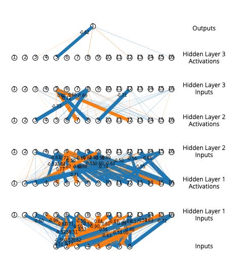
While this time the model was not able to learn a sparse weight matrix that exactly reflected our
labelling function (see Figure 15), the model was again able to leverage the XNORAIL activation
function to significantly outperform an identical model utilizing the ReLU activation function.
(a) XNORAIL learned weight matrix (b) ReLU learned weight matrix
Figure 15: Training results, regression experiment on second synthetic dataset
We found that a simple model with three hidden layers, each with eight neurons, utilizing XNORAIL
was able to go from a validation RMSE of 0.287 at the beginning of training to a validation RMSE of
0.016 after 100 epochs. Comparatively, an identical model utilizing the ReLU activation function was
only able to achieve a validation RMSE of 0.271 after 100 epochs. In order for our ReLU network
to match the validation RMSE of our 8-neuron-per-layer XNORAIL model, we had to increase the
model size by 32 times to 256 neurons at each hidden layer.
2
We hypothesize that, because our XNORAIL activation function reduces the number of hidden layer neurons
by a factor of k, having a reduced number of neurons at each layer creates a bottleneck in the later layers of the
network which restricts the amount of information that made its way through to the final layer
21You can also read