Longitudinal forces evaluation of SNCF trains
←
→
Page content transcription
If your browser does not render page correctly, please read the page content below
Challenge C: Increasing Freight capacity and services

            Longitudinal forces evaluation of SNCF trains

                                        Cantone L.1, Durand T.2

1
  Università di Roma “Tor Vergata”, Dipartimento di Ingegneria Meccanica, via del Politecnico, 1 –
00133 Roma
2
  Pole Rolling stock body and developments, CIM of SNCF, 4 allée des Gémeaux, 72000 Le Mans

1 Introduction
The investigation of Longitudinal Forces (hereafter LF) exchanged between two consecutive vehicles
of a train has a paramount importance in assessing train compositions, since it affects train suitable
length, applicable traction power, load capacity and permissible speed, especially for heavy hauled
freight trains. Wrong decisions concerning these parameters result in an increased risk of accidents
due to derailments and/or train disruptions, which produce, as a consequence, damage of wagons, of
goods, of railway infrastructure and service loss.
In order to increase the efficiency of freight train transportation, the Union Internationale des Chemins
de Fer (UIC) has decided to enhance the Train Dynamic (TrainDy) software, developed by the
University of Rome «Tor Vergata», with financial support from Faiveley Transport Italia. The idea at
the basis of TrainDy’s development is not providing industry professionals with a new software, more
or less evolved as compared to previous ones (see [1]-[2] for a few recent papers on train longitudinal
dynamics), but rather constituting a common platform (capable to compute the longitudinal as well as
the three-dimensional dynamics of a train, including also the study of vehicle/track interaction), that is
open to contribution from professionals themselves and industry researchers. Such format totally
complies with UIC’s policies, and best meets Europe’s expectations in terms of increasing high-
capacity transport of goods by rail, also aiming at a full, complete trans-national inter-operability. This
makes TrainDy suitable to meet various needs of railway companies: from train composition
assessment to train driver training. The software basically consists of two modules: the pneumatic
module and the dynamic module, which can run simultaneously or separately, according to the
specific analysis. This paper deals only with the longitudinal module of TrainDy, which has been
officially certified by the UIC in January 2009.
The pneumatic module, which computes the air pressure in general brake pipe and in brake cylinders,
constitutes one of the key features of TrainDy; in literature there are several papers dealing with the
same issue: among them, [3]-[5] deserve a specific mention, as in those works the fluid dynamics
model developed in [6] is applied successfully to pneumatic brakes used on trains. The approach
followed by TrainDy further generalizes those models and differs from the model proposed in [7],
which is based on the facilities of Simulink. Compared to the latter model, TrainDy has at least equal
numerical accuracy, but also higher numerical efficiency. The pneumatic module of TrainDy can
easily handle braking and releasing manoeuvres for long trains with more than one active locomotive
[8]; this means that TrainDy, also thanks to its dynamic module – featuring exceptional accuracy as
well as reliable calculation efficiency – allows to efficiently investigate the longitudinal dynamics of
very long trains.
TrainDy is programmed in MATLAB and it has been subjected to a validation and verification process
by the UIC Experts Group. The core of this validation was split into two main steps: pneumatic
validation and dynamic validation. Pneumatic validation led to mapping the most widely used
European braking devices. It provides a 10% maximum error rate, comparing the pressures in the
braking cylinders with the experimental data from real trains. The needed test run data were provided
by the European Railways Companies DB AG, SNCF and Trenitalia. In addition, Faiveley Transport
Italia has provided experimental results of their own full scale hardware train brake simulator.
Dynamic validation was carried out by matching the longitudinal forces and the stopping distances
both with the software previously used by UIC and, directly, against experimental data. The used
experimental test campaigns enabled to study the longitudinal forces for long freight trains, also with
more than one active locomotive (distributed braking).

                                                    1
Challenge C: Increasing Freight capacity and services
SNCF, as the three main European Railways Companies (DB AG, SNCF, Trenitalia), supports the
TrainDy project. SNCF, and more particularly the CIM (Centre d’Ingénierie du Matériel) based at Le
Mans, carries out studies with this software for its customers. TrainDy is used at SNCF for:
Feedback studies : it consists in trying to understand why a particular incident like train
disruption, derailment or specific wear has occurred. The engineers try to reproduce the
event with the software and compare the results of LF with critical limits.
Statistic studies : it consists in validating a new exploitation by proving the corresponding
new system is at least as safe as a reference system which is considered safe. For example,
the UIC is building a procedure which should be used to calculate the probability of
derailment of a system.
Investigation studies : it consists in exploring the feasibility of new solutions which are
advantageous for customers because it optimizes its production.
The chapter 3 of this paper presents an example of investigation study linked to the risk of train
disruptions.
2 Models
Hereafter it is reported the short summary of the main models used to properly compute LF between
consecutive vehicles. The mathematical models are particularly suited to the situation of the freight
trains commonly circulating in Europe, for which it is necessary to firstly evaluate the air pressure in
brake cylinders (pneumatic module), then transforming these pressures into brake forces (brake
module) and, lastly, solving the non-linear longitudinal dynamics of the train (dynamic module).
2.1 Pneumatic module
The pneumatic module – the basic module of the software – has been extensively described in [8];
here we shall only point out that its main devices (Brake Pipe, Driver’s Brake Valve, Control Valve –
completed with Acceleration Chambers (AC)– Brake Cylinders and Auxiliary Reservoirs, as shown in
Fig. 1) have been modeled using one or more equivalent and significant parameters. It’s important to
emphasize the meaningfulness of the parameters used from the pneumatic module, since this lets to
the “Power User” the possibility to adjust those parameters in order to quickly reproduce the
pneumatic behavior of the real equipments.
2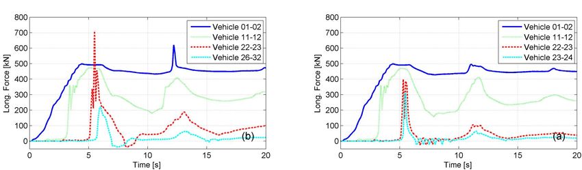
Challenge C: Increasing Freight capacity and services
Fig. 1 Sketch of train pneumatic system.
Modeling of the main brake devices can be outlined as follows:
Brake Pipe (BP) is modeled as a circular pipe with variable diameter to allow the modeling of hose
couplings between two adjacent vehicles; the governing quasi one-dimensional Navier-Stokes
equations are shown in [8]. Distributed and concentrated pressure losses are considered,
respectively, by Colebrook formulation and equivalent tuning coefficient. Length and diameters of
the brake pipe are the same as real data. The governing Navier-Stokes equations are as follows:
uS m
u
t x S x Sdx
u 1 p u u m
(1) u
t x x D Sdx
q q T T uS u m 1 1
u r r 4 T cv r Tl ul2 q
t x x S x D D Sdx 2
where is the density, u axial velocity, p pressure, T temperature and all of them must be
considered as mean values on the general cross-section S of diameter D and abscissa x; q is the
D u2
specific energy, cv specific heat at constant volume, sgn u f K takes into
dx 2
account the dissipative sources (there, f is the distributed coefficient of pressure loss, K
concentrated coefficient of pressure loss and sign function); T is the exchanged thermal
flux, r gas constant, m in-flow or out-flow mass flux; and, finally, subscript l refers to lateral
quantities, which has to be computed by imposing the right boundary conditions.
Eqs (1) have been numerically solved using a third order Taylor expansion of , u and q. The spatial
domain has been discretized using a constant mesh of 1 m and the identification of all equivalent
parameters has been performed on this set up.
3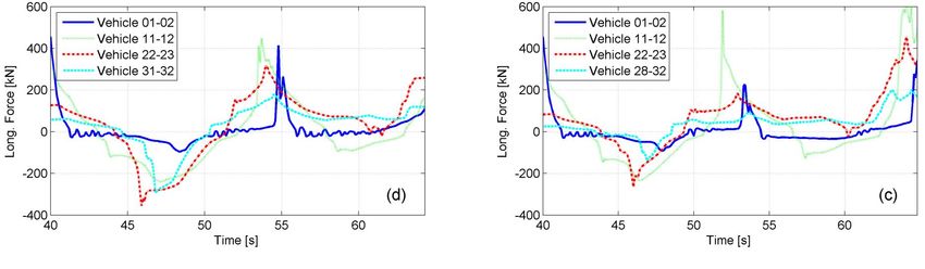
Challenge C: Increasing Freight capacity and services
Last wagon
First wagon
Fig. 2 Pressure in BP for several values of equivalent nozzle diameter connecting BP with AC
and several values of AC volume: (a), reference; (b), diameter only increasing; (c), volume only
increasing; (d), both increasing.
Driver’s Brake Valves (DBVs) are modeled as nozzles with fixed diameter: one for emergency
brake, another for service brake and a third for releasing, since pneumatic circuits are different for
these types of operations. Once the general parameter is identified for one test, its value is
satisfactory for every test and this means that its value can be associated to the target specific
equipment, which is in this way “mapped” in TrainDy. Note that for service brake, only one
diameter needs to be identified, even if the manoeuvre target pressure is different.
Acceleration Chambers (ACs) of the distributors are modeled via their volume and the diameter of
an equivalent nozzle between the AC and the BP.
As concerns Brake Cylinders (BCs), equivalent coefficients are employed to approximate the
application stroke and in-shot function (the first phase of braking [11]), in order to avoid a complex
and useless (for the focus of TrainDy) 3D fluid-dynamic modeling. After this phase, brake cylinders
are filled considering static transfer functions of distributors (or Control Valves) and limiting curves
of a specific brake regime.
Auxiliary Reservoirs (ARs) of the distributors are modeled as volumes connected to the brake pipe
via a nozzle with variable diameter.
Considering that TrainDy pneumatic module needs several coefficients to be tuned, their
determination by a trial-and-error procedure might appear very time consuming. Nevertheless, since
each parameter has a known physical meaning and a precise consequence on the BP and BCs
pneumatics, the parameter determination turns out to be quite simple and fast. As an example of the
tuning procedure, see Fig. 2 showing the emptying of the brake pipe on a 400 m long train with an
active locomotive at its head, performing emergency braking: in this case, air pressure time evolution
is represented only for vehicles 1, 2, 10, 18 and 21 (last vehicle). As usual, in order to properly identify
the equivalent nozzle diameter connecting BP with ACs and their volume, it is necessary to focus on
the initial air pressure jump, which is clear for last vehicles. Fig. 2 shows the influence of AC volume
and AC equivalent nozzle diameter on brake pipe emptying. In Fig. 2 (a), volume of ACs is set to 0.9 l
and the equivalent nozzle diameter is set to 3 mm. By increasing the equivalent nozzle diameter to 7
mm, Fig. 2 (b), air pressure drop is faster and its «rebound» is more evident. By increasing AC
volume to 1.5 l – see Fig. 2 (c), air pressure drops more significantly than in Fig. 2 (a) because it is
necessary to fill a greater volume and their filling ends after 3 s (instead of 2.5 s). Lastly, by increasing
4
Challenge C: Increasing Freight capacity and services
the equivalent nozzle diameter from 3 mm to 7 mm, Fig. 2 (d), the pressure drop becomes faster,
although its magnitude remains the same as in Fig. 2 (c). By matching all the results it is clear that AC
volume determines the local air pressure minimum, whereas the equivalent nozzle diameter
influences air pressure «rebound».
2.2 Traction, Brake and Coupling modules
This section briefly describes the other modules of TrainDy: traction, brake and coupling.
The traction module is essential for assessing the longitudinal dynamics of trains, considering, for
example, the forces at the draw gears, or the train configurations with more than one locomotive (the
so called “distributed traction” or “distributed power” [9], [10]), in order to find the position of the
remote locomotives which can lead to a reduction of LF. The traction module is also useful to
reproduce undesired scenarios that have occurred during accidents. By mean of this module, for
example, it is possible to compute LF when emergency braking occurs immediately after traction (high
compression forces at buffers) or, for trains with two locomotives, when an emergency brake is
activated at the back of the train while traction is still being applied at the front (causing high traction
forces at draw gears that may provoke train disruption). Of course, in order to manage such
scenarios, the behavior of each locomotive must be independent and, in order to reproduce an
accident, it is necessary to control this behavior with respect to time, position and speed.
Traction force is directly modeled in TrainDy using the force-speed diagram of the locomotive, set in
input as a series of points; moreover, traction force can be imposed as a general function of time.
Then, in order to have a versatile module, the force gradient during traction application and removal
can be also imposed and, lastly, overall power can be linearly changed from zero to maximum power.
Of course, the electro-dynamic brake is also managed: this means that locomotives may have both
pneumatic and electro-dynamic braking at the same time.
Concerning pneumatic braking of vehicles, the two most common brake systems are implemented:
block brake and disk brake; moreover, an auto-continuous device and an empty-load device are also
available, so that the braked weight percentage of vehicle changes continuously with vehicle load, or
it shows a discontinuity due to “empty” and “loaded” settings. Computation of brake force is carried
out according to UIC 544-1 [12] and it is possible to evaluate the braking force both from the design
brake parameters (rigging ratio, rigging efficiency, distance of disk pad from wheel axis, etc.) and from
the braked weights.
For both brake systems (block and disk) it is possible to impose a desired speed evolution for friction
coefficient, as sketched in Fig. 3 (a) and (b) , where two examples are reported, for block and disk
brakes, respectively.
For block brakes, the friction coefficient depends on speed and specific pressure (Psp) between block
and wheel; whereas, for disk brakes, it is only a function of speed. The TrainDy software allows the
implementation of user-defined friction laws as well as mathematical laws, as described in [13]. For
instance, a good matching with experimental results has been obtained by using Karwatzki law, in
order to model the friction coefficient for block brakes:
16
Fk 100
g V 100
(2) (V , Fk ) 0.6
80
Fk 100 5V 100
g
where: Fk [kN] is the total normal force between block and wheel, V [km/h] is vehicle speed, g is
gravitational acceleration [m/s]. For disk brake, a constant value of 0.35 has been used for friction
coefficient, during the validation process.
5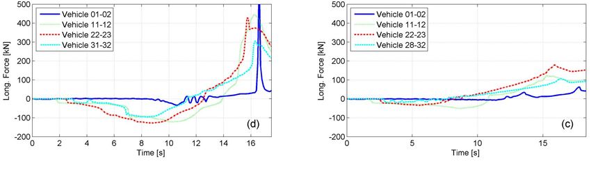
Challenge C: Increasing Freight capacity and services
Fig. 3 Examples of speed evolution for block brake (a) and disk brake (b) friction coefficients.
In (a) Psp is the specific pressure between wheel and shoe.
Running resistance is evaluated as follows [14]:
(3)
FRes 1.1 0.00047 v2 g mv cos [N]
where: v is vehicle speed in [m/s], mv is vehicle mass in [ton] and is track slope [rad].
Buffers and draw gears are modeled by their force-stroke characteristics, while considering a friction
model for damping - i.e. when relative speed is in the interval between load velocity (v load) and unload
velocity (vun-load) - the exchanged force is computed as:
(4) FLong xrel , vrel cvrel Fun load xrel 1 cvrel Fload xrel
where x rel and vrel are the relative displacement and speed, respectively, of consecutive vehicles,
c v rel coefficient is represented by a third order polynomial connecting loading curve ( Fload ) to
unloading curve ( Fun load ).
i m o m
(5) xrel xrel DL , xrel xrel DL
where, is the relative angle of consecutive vehicles and DL is the half transversal distance of
buffers.
A new, more refined, buffer/draw gear model is being developed, as described in [15].
Once forces on each vehicle have been evaluated, the following non-linear equations of motion can
be solved:
(6)
a M 1 FLong xrel , vrel FBraket , v FLoco t , v FRes v
where: M is the mass matrix which is lumped and time invariant, FBrake are the brake forces acting for
each vehicle, FLoco are the traction forces (or even braking forces during an electro-dynamic braking)
of locomotives, a is acceleration and t is time. Note that vehicle mass is taken into account also for
rotating inertia, that is: mv 1 Tare Load , where is the fraction of rotating inertia.
Equations (6) are solved using MATLAB Ordinary Differential Equations (ODEs) solver: after an
investigation addressed to balance the accuracy and the computational efficiency on several test
cases, a variable time step integrator for stiff problems is employed, namely ode15s [16], using a
relative tolerance of 10-6 and providing a pattern for the Jacobian.
3 Train disruption risk at SNCF
3.1 Overall view
The limited weights of the freight trains are defined in Technical Specifications (hereafter TS), kind of
regional code for trains. The weights of freight trains are not only fixed by the limiting capacities of the
engines (in terms of maximal forces and heat stresses) but also by the risk of train disruption: this
limit, existing in case of use of multiple locomotives in front of the train, is generally determined thanks
to this formula which is based on static mechanic principles:
6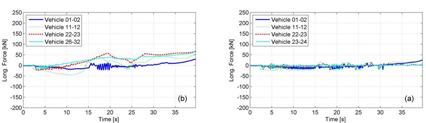
Challenge C: Increasing Freight capacity and services
Fd
(7) Wdr
rt
Where:
Wdr is the limited Weight due to Disruption Risks [t]
Fd is the theoretical static force necessary to disrupt a drawgear [daN]
rt is the specific resistance to be overtaken to start the train [daN/t]. rt depends on the characteristic
ramp i (e.g. i ~30 ‰ in the Alpes to go from France to Italy) of the route defined in the TS
is a safety coefficient.
In order to optimize the limit Wdr in the TS, the Railway Company has to change one of the three
factors in equation (7). That would mean:
Increasing Fd: this can be only done by modifying the screw coupling resistance which is the
weakest mechanic point inside the couplings. Standard screw coupling which equip wagons are
defined to resist to 850 kN, but some enforced screw coupling resist to 1350 kN. In Italy, screw
coupling are designed to resist to 1020 kN according to [17] The gain could be interesting but is
expensive because all the wagons of the wished exploitation would need to be equipped with new
drawgears. Now, to modify the complete drawgear it is necessary to change screw couplings,
hooks and drawbars.
Lowering rt : this parameter is linked to the wagon and the locomotive characteristics. For
example, new locomotives set up with new designed asynchronous engines should permit to
optimize this level with respect to old locomotives. Nevertheless, the validation of such a change
demands long and costly tests for an optimization that can be small.
Lowering : historically this parameter has been fixed to 2.35 for the common trains. It considers
both the dynamic influence of the train and the ratio (Disruption Force/Elastic Limit Force) for the
Elastic Limit force: it is considered as a good criterion not to overtake in case of repeated loads.
Here is the most interesting lever in terms of costs and time: a technical study, made with a tool as
accurate as TrainDy, can demonstrate that a reduction of , in some specific cases, does not
increase the risk of train disruption and does not reduce the regularity of the global traffic.
For instance, in the TS, for homogeneous freight heavy trains named “whole” trains, rules are less
restrictive because these trains are supposed to generate less longitudinal dynamic forces: the
coefficient is fixed to 2.2, which increases by 7% the limited weight of the train with respect to a
common train.
3.2 Methodology used for the specific issue of whole trains
The use of the 2.2 coefficient would allow Fret SNCF to reduce its quantity of trains and increase its
productivity. As the characteristics of the “whole” train are not completely defined inside the rules, the
idea is to complete a homogeneous train with slightly heterogeneous one and consider this new train
as a “whole” train (see the distribution mass cases 1) – 4) hereafter). Therefore, the opinion of the
engineering rolling stock center CIM was requested on these two planned exploitations:
- Case 1: Addition of an empty train on a fully loaded one,
- Case 2: Train composed of loaded wagons which are not of the same type.
For case 2, an advice based on an expert judgment was given: there is no problem to consider case 2
trains as “whole” trains if the dispersion between the braking of the first and the second part of the
train is low.
For case 1, CIM decided to treat with TrainDy the feasibility of this wished operation.
First of all, the feedback of the CIM concerning the problematic of train disruptions is very global and
does not reveal typical causes, positions and origins in train disruptions: they can occur in the first
part of a train as well as among the last couplings, they sometimes happen in starting procedures but
often in braking ones. Nevertheless the analysis of the failures shows two interesting points:
Most of them are brutal disruptions not caused by repetitive forces above the acceptable
limits in case of repeated solicitations
The type of locomotive and its traction capacity to accelerate is an important factor in the
disruptions.
That is why it was necessary to lead the analysis of various driving manoeuvres while studying
different compositions.
7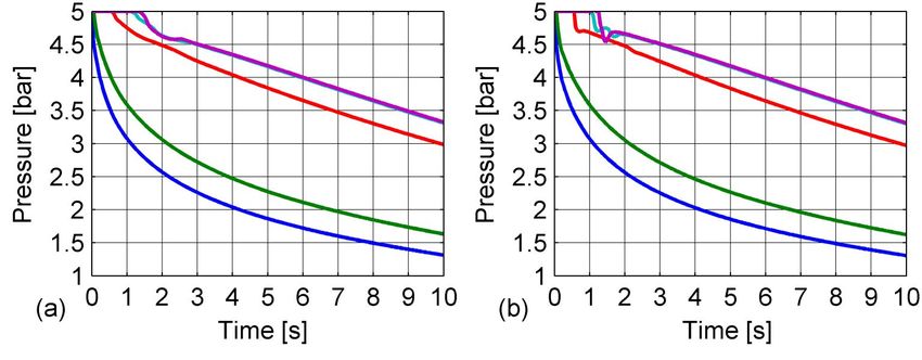
Challenge C: Increasing Freight capacity and services
The compositions investigated, corresponding to the need of the Customer, were the following (the
mass of the train is without locomotives):
a) A 2000 t “whole” train with a mass of 2000 t formed with 22 full loaded wagons (90 t)
b) A 2200 t train set up with 23 loaded wagons (90 t) and 5 empty wagons (20 t)
c) A 2200 t train set up with 22 loaded wagons (90 t) and 9 empty wagons (20 t)
d) A 2200 t train set up with 22 loaded wagons (80 t) and 18 empty wagons (20 t)
The first configuration above represents the reference while the other ones are envisaged possibilities
to optimize the exploitation with a new safety coefficient.
For each of these compositions, the following driving manoeuvres, decided from the feedback of
SNCF, were calculated :
A. EB : Emergency braking without initial tension at the drawgears (initial velocity 30 km/h)
B. SB 1b : Service braking released with 4 bar in the general pipe (initial velocity 60 km/h)
C. EB Traction : Emergency braking with initial tension at the drawgears created by locomotive
traction (initial velocity around 35 km/h)
D. Rapid Traction : Rapid acceleration of the train considering the fastest capacities of the
Multiple Units (MU) of the locomotives (Total traction force provided by the engines increasing
linearly from 0 kN to 500 kN in 4 seconds)
The percentages of braking weight considered for the simulations were the following: 60 % for a full
loaded wagon of 90 t, 67.5 % for a loaded wagon of 80 t and 120 % for an empty wagon.
The elastic devices used for the calculation correspond to Caoutchouc - Metal materials which usually
equip French wagons.
3.3 TrainDy calculations - analysis
The first results here presented deal with the SB manoeuvres for the 4 compositions a)-d) listed
above: Fig. 4 shows the results in terms of longitudinal forces for only some elastic couplings for sake
of clearness.
Fig. 4 Service braking. (a)-(d) according to the previous bullet list a)-d)
The maximum LF generated during a normal service braking for a “whole” train (a) are less than 50
kN. The homogeneity of the braking power (brake weight percentage) along the train explains these
low values which are of course completely acceptable with respect to drawgear conception: the tiring
limit is never overtaken. With 5 to 10 empty vehicles behind a full loaded train, case b) and c),
respectively, the Longitudinal Compressive and Traction Forces (hereafter LCF and LTF) increase but
stay under tiring limits (100 kN in compression and 150kN in traction).
8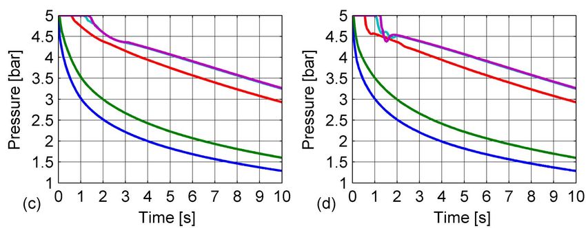
Challenge C: Increasing Freight capacity and services
It is not the case when 20 empty wagons are added behind the loaded ones: a LCF of 200 kN is
reached whereas 250 kN is approximately the maximum LTF (see Fig. 4 d)).
In shunting areas, a LCF superior to 200 kN can theoretically lead to a derailment. And 250 kN is over
the tiring limit for which the Standard screw couplings are manufactured (see EN 15566) in terms of
life cycle limits. Considering that a normal service braking is a nominal event, the addition of too many
empty wagons can be prejudicial for materials in the long term, so it must be avoided.
Fig. 5 presents the results of EB manoeuvres for the 4 compositions a)-d) calculated with TrainDy:
Fig. 5 Emergency braking. (a)-(d) according to the previous bullet list a)-d)
When an emergency braking occurs, there is the same global qualitative evolution of LF from a) to d),
as it has been seen for the service braking. Nevertheless, it is a fact that some LTF peaks can be
created which threaten the integrity of the freight train (in terms of possible train disruptions). The
calculations are usually not sufficient to determine, with the requested accuracy, the reached values,
in case of instantaneous peak over 500 kN; anyway, the calculations can be considered as good
means to represent the risk. Indeed, tests on real trains have shown that these dynamic peaks exist
and explain, most of time, the trains disruptions.
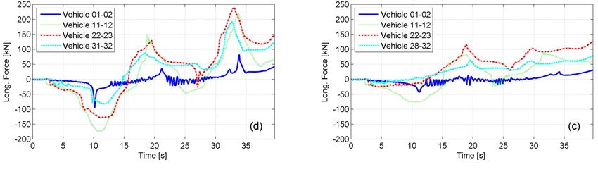
Fig. 6 presents the results of EB manoeuvres with tension in drawgears, due to a locomotive
acceleration, for the 4 compositions calculated with TrainDy.
9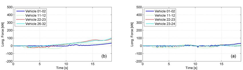
Challenge C: Increasing Freight capacity and services

    Fig. 6 Emergency braking after traction. (a)-(d) according to the previous bullet list a)-d)

Also in this case, there are some peaks both in LCF and in LTF and their amplitudes are usually
bigger than in case of EB. Also for this type of manoeuvre, there is the same global qualitative
evolution from a) to d), emphasizing that the longitudinal dynamics is deeply determined by mass
distribution.

Fig. 7, finally, shows the LF caused by a Rapid Traction, for the 4 compositions a)-d), again calculated
with TrainDy.

                                                  10
Challenge C: Increasing Freight capacity and services
Fig. 7 Rapid Traction. (a)-(d) according to the previous bullet list a)-d)
Some LTF higher than 500 kN are reached for each configuration. It means the risk is present even
for the whole trains, but such risky conditions have been obtained for manoeuvres that are considered
as “degraded”. Driving rules insist on the way to start a train without damaging the drawgear. So they
should not be practiced by drivers during normal exploitations.
4 Closing remarks
The calculations show that the dangerous event of train disruptions exists both for train presently in
exploitation and for new mixed empty/full loaded trains wished in the near future. However for “whole”
trains, this risk only appears in case of degraded conditions whereas damages on drawgears, at least
by progressive solicitations, are possible in nominal conditions for the new operating conditions.
For nominal conditions, it can be assessed that the reduction of the safety coefficient , for a train
constituted with more than 10 empty wagons behind a “whole” train, would certainly increase the risk
of freight train disruptions. And this risk would exist even in case of =2.35 in the case of this specific
operation.
Finally, CIM has agreed to reduce to 2.2 the safety coefficient but has proposed to limit the quantity
of empty wagons. Moreover CIM has recommended to warn and inform drivers about the risks
caused when operating these new train compositions.
The utility of a tool like TrainDy cannot be contested. It helps to demonstrate the danger of new and
actual operations. Besides, it mainly affords to optimize the length and weight rule limits of freight
trains. The gains for railway productivity are important and could certainly be considerable if the
Customers needs and the Specialists proposals are harmonized and if new tools are developed for
TrainDy.
For instance, in a close future, we can imagine some driving simulators including real time LF
calculation, showing the drivers the best way to operate in normal and critical situations.
11Challenge C: Increasing Freight capacity and services
5 References
[1] Chou M., Xia X.; Kayser C., “Modelling and model validation of heavy-haul trains equipped
with electronically controlled pneumatic brake systems” Control Engineering Practice, v 15,
n 4, March, 2007, p 501-509.
[2] Belforte P., Cheli F.; Diana G.; Melzi S., “Numerical and experimental approach for the
evaluation of severe longitudinal dynamics of heavy freight trains”, Vehicle System
Dynamics, v 46, n SUPPL.1, In Memory of Joost Kalker, 2008, p 937-955.
[3] Murtaza, M. A.; Garg, S.B.L.; Brake modelling in train simulation studies. Proc. Inst. Mech.
Engrs, 203(F2), 1989, p. 87-95.
[4] Murtaza, M. A.; Garg, S.B.L.; Transient performance during a railway air brake release
demand. Proc. Inst. Mech. Engrs, 204(F1), 1990, p. 31-38.
[5] Murtaza, M. A.; Garg, S.B.L.; Parametric study of railway air brake system. Proc. Inst. Mech.
Engrs, Part F, 206(F1), 1992, p. 21-36.
[6] J. E. Funk, T. R. Robe, “Transients in pneumatic transmission lines subjected to large pressure
changes”, International Journal of Mechanical Science, 1970, Vol. 12, pp. 245-257.
[7] L. Pugi, M. Malvezzi, B. Allotta, L. Banchi, P. Presciani, "A parametric library for the
simulation of UIC pneumatic braking system", Proc. of the IMechE, Journal of Rail and Rapit
Transit, vol. 218, part F, pp.117-132.
[8] L. Cantone, E. Crescentini, R. Verzicco, V. Vullo, “A numerical model for the analysis of
unsteady train braking and releasing manoeuvres”, Proc. IMechE, Part F: J. Rail and Rapid
Transit, 2009, 223 (F3), 305-317.
[9] Parker, C.W., “Design and Operation of Remote Controlled Locomotives in Freight Trains”,
Railway Engineering Journal, Jan. 1974, pp 29-38.
[10]Simon Iwnicki, Handbook of Railway Vehicle Dynamics (Eds), Taylor&Francis, 2006.
[11]UIC 540-0 “Freins a air comprimé pour trains de marchandises et trains de voyageurs”, UIC,
Paris, France, 3° Edition, 01.01.1982.
[12]UIC 544–1. Brakes – braking power, 4th edition October 2004, Paris, France.
[13]T. Witt, “Integrierte Zugdynamiksimulation für den modernen Güterzug”, Dissertation
Institut für Verkehrswesen, Eisenbahnbau und –betrieb, Universität Hannover, Hannover
2005.
[14]R. Panagin, “La Dinamica del Veicolo Ferroviario” Levrotto & Bella, Torino 1997.
[15]L. Cantone, D. Negretti, “Modellazione dinamica disaccoppiata dei respingenti ferroviari”,
AIAS 2009 9-11 Settembre Torino, 2009.
[16]Shampine, L. F., “Numerical Solution of Ordinary Differential Equations”, Chapman & Hall,
New York,1994.
[17]EN 15566. European Standard - Railway applications - Railway rolling stock - Draw gear and
screw coupling, January 2009
12You can also read