Low-level liquid cloud properties during ORACLES retrieved using airborne polarimetric measurements and a neural network algorithm
←
→
Page content transcription
If your browser does not render page correctly, please read the page content below
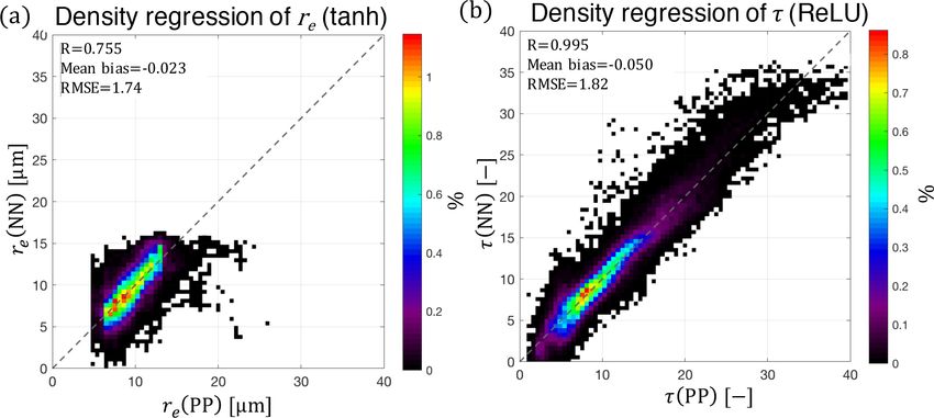
Atmos. Meas. Tech., 13, 3447–3470, 2020
https://doi.org/10.5194/amt-13-3447-2020
© Author(s) 2020. This work is distributed under
the Creative Commons Attribution 4.0 License.

Low-level liquid cloud properties during ORACLES retrieved
using airborne polarimetric measurements and a
neural network algorithm
Daniel J. Miller1,2 , Michal Segal-Rozenhaimer3,4,5 , Kirk Knobelspiesse1 , Jens Redemann6 , Brian Cairns7 ,
Mikhail Alexandrov7,8 , Bastiaan van Diedenhoven7,9 , and Andrzej Wasilewski7,10
1 NASA   Goddard Space Flight Center, Greenbelt, MD, USA
2 UMBC    Joint Center for Earth Systems Technology, Baltimore, MD, USA
3 NASA Ames Research Center, Moffett Field, CA, USA
4 Bay Area Environmental Research Institute, Moffett Field, CA, USA
5 Department of Geophysics, Porter School for the Environment and Earth Sciences, Tel Aviv University, Tel Aviv, Israel
6 School of Meteorology, The University of Oklahoma, Norman, OK, USA
7 NASA Goddard Institute for Space Studies, New York, NY, USA
8 Department of Applied Physics and Applied Mathematics, Columbia University, New York, NY, USA
9 Center for Climate System Research, Columbia University, New York, NY, USA
10 SciSpace LLC, Broadway, New York, NY, USA

Correspondence: Daniel J. Miller (daniel.j.miller@nasa.gov)

Received: 29 August 2019 – Discussion started: 16 September 2019
Revised: 5 May 2020 – Accepted: 10 May 2020 – Published: 29 June 2020

Abstract. In this study we developed a neural network (NN)        rithms. This approach could be particularly advantageous for
that can be used to retrieve cloud microphysical proper-          more complicated atmospheric retrievals – such as when an
ties from multiangular and multispectral polarimetric remote      aerosol layer lies above clouds like in ORACLES. For RSP
sensing observations. This effort builds upon our previous        observations obtained during ORACLES 2016, comparisons
work, which explored the sensitivity of neural network in-        between the NN and standard parametric polarimetric (PP)
put, architecture, and other design requirements for this type    cloud retrieval give reasonable results for droplet effective
of remote sensing problem. In particular this work introduces     radius (re : R = 0.756, RMSE = 1.74 µm) and cloud optical
a framework for appropriately weighting total and polar-          thickness (τ : R = 0.950, RMSE = 1.82). This level of sta-
ized reflectances, which have vastly different magnitudes and     tistical agreement is shown to be similar to comparisons be-
measurement uncertainties. The NN is trained using an artifi-     tween the two most well-established cloud retrievals, namely,
cial training set and applied to research scanning polarimeter    the polarimetric and the bispectral total reflectance cloud re-
(RSP) data obtained during the ORACLES field campaign             trievals. The NN retrievals from the ORACLES 2017 dataset
(ObseRvations of Aerosols above CLouds and their intEr-           result in retrievals of re (R = 0.54, RMSE = 4.77 µm) and τ
actionS). The polarimetric RSP observations are unique in         (R = 0.785, RMSE = 5.61) that behave much more poorly.
that they observe the same cloud from a very large num-           In particular we found that our NN retrieval approach does
ber of angles within a variety of spectral bands, resulting in    not perform well for thin (τ < 3), inhomogeneous, or broken
a large dataset that can be explored rapidly with a NN ap-        clouds. We also found that correction for above-cloud atmo-
proach. The usefulness of applying a NN to a dataset such         spheric absorption improved the NN retrievals moderately –
as this one stems from the possibility of rapidly obtaining       but retrievals without this correction still behaved similarly
a retrieval that could be subsequently applied as a first guess   to existing cloud retrievals with a slight systematic offset.
for slower but more rigorous physical-based retrieval algo-

Published by Copernicus Publications on behalf of the European Geosciences Union.
3448                D. J. Miller et al.: Cloud property retrievals during ORACLES using a polarimetric neural network

1   Introduction                                                   we will focus on in this study (Werdell et al., 2019). From
                                                                   a passive cloud remote sensing perspective, the persistence
Advancing the scientific understanding of aerosol–cloud in-        of ACA in the ORACLES study region can represent a diffi-
teractions is imperative for forming a more complete pic-          cult and sometimes confounding issue. Cloud microphysical
ture of the Earth climate system. These interactions are re-       retrievals which do not consider the presence of the aerosol
sponsible for large uncertainties in our understanding of an-      above the cloud can suffer biases due to the impact of ab-
thropogenic climate forcing (IPCC, 2013). The uncertainty          sorption of the overlying BB aerosols in shortwave spectral
primarily stems from the semidirect and indirect effects of        bands. Most notably, this was found to be the case for the
aerosols on clouds (Wilcox, 2010, 2012; Lu et al., 2018),          Moderate Resolution Imaging Spectroradiometer (MODIS)
which have been found to have significant yet uncertain cli-       cloud retrieval product (Meyer et al., 2013). It is possible to
mate impacts (Sakaeda et al., 2011).                               correct for this impact, but an assumed aerosol model is re-
   Not many other regions of the world have as consistent          quired to constrain the otherwise unknown optical properties
aerosol–cloud interactions as the marine boundary layer of         of the aerosol. On the other hand, there are some ACA re-
the southeast (SE) Atlantic Ocean. This region is dominated        trieval methods that attempt to simultaneously retrieve full
by a semipermanent subtropical stratocumulus (Sc) deck that        aerosol and cloud properties of ACA scenes. However, the
regularly interacts with significant biomass burning (BB)          existing techniques each still exhibit shortcomings when it
aerosols originating from natural and anthropogenic (agri-         comes to constraining aerosol absorption properties (e.g.,
cultural) fires in central Africa during austral spring (July–     single-scattering albedo or complex refractive index) and
October) (Zuidema et al., 2016). The aerosols are lofted           thus can result in an inaccurate representation of the direct
into the mid-troposphere over land before being transported        radiative effect of ACA (Knobelspiesse et al., 2015; Yu and
by large-scale circulation, eventually arriving above the ma-      Zhang, 2013). One of the more promising approaches takes
rine stratocumulus deck (Adebiyi and Zuidema, 2016). This          advantage of the large information content of multispectral,
leads to near-persistent above-cloud aerosol (ACA) condi-          multiangular, and polarization observations. The vast infor-
tions that have consequential impacts on the radiative budget      mation content of polarimetric observations provides ample
via direct radiative effects (i.e., enhanced aerosol absorption;   opportunities to simultaneously retrieve aerosol and cloud
Meyer et al., 2013; Zhang et al., 2016) and semidirect ra-         properties. This methodology has been applied to both or-
diative effects that can induce numerous cloud adjustments         bital (Waquet et al., 2009, 2013) and suborbital field cam-
(e.g., increased vertical stability, burn off, etc.; Koch and      paign observations (Knobelspiesse et al., 2011b; Xu et al.,
Del Genio, 2010; Wilcox, 2012). As a result of this unique         2018).
environment, the SE Atlantic region has become the focus              In this study, we make use of polarimetric observations
of sustained research efforts. In addition to orbital observa-     obtained using the research scanning polarimeter (RSP) dur-
tions, several international field campaigns have overlapped       ing ORACLES 2016 and 2017 field campaigns. The RSP
with one another to explore this region, including CLARIFY         is the airborne prototype for the aerosol polarimetry sen-
(UK Met Office, CLoud-Aerosol-Radiation Interactions and           sor (APS) built for the NASA Glory mission (Mishchenko
Forcing: Year 2016; Zuidema et al., 2016), AEROCLO-SA              et al., 2007; Peralta et al., 2007; Persh et al., 2010). While
(French National Research Agency, AErosol RadiatiOn and            Glory did not successfully enter orbit due to a launch failure,
CLOuds in Southern Africa; Formenti et al., 2019), ONFIRE          the pair of RSP instruments, denoted RSP1 and RSP2, con-
(US National Science Foundation, Observations of Fire’s Im-        tinue to make observations and have been deployed on over
pact on the Southeast Atlantic Region), LASIC (US Depart-          25 field missions in the last 20 years. The instruments her-
ment of Energy, Layered Atlantic Smoke Interactions with           itage, accuracy, and measurement characteristics make it well
Clouds; Zuidema et al., 2018), and ORACLES (NASA, Ob-              suited for observations of clouds (Alexandrov et al., 2012a,
seRvations of Aerosols above CLouds and their intEractionS;        b; van Diedenhoven et al., 2016, 2013; Sinclair et al., 2017),
Zuidema et al., 2016). The last of these campaigns is the fo-      aerosols (Chowdhary et al., 2001; Chowdhary and Cairns,
cus of this study.                                                 2002; Chowdhary et al., 2012; Knobelspiesse et al., 2011a,
   To study this region, numerous state-of-the-art in situ and     b; Wu et al., 2015, 2016; Stamnes et al., 2018), the ocean
remote sensing instruments have participated in ORACLES            (Chowdhary et al., 2006; Chowdhary et al., 2005b, a; Otta-
flights in three deployments each austral spring from 2016 to      viani et al., 2012), and snow (Ottaviani et al., 2015). In partic-
2018. As a consequence, the ORACLES dataset offers the             ular the cloud retrieval products of RSP are well established
opportunity to test and develop new remote sensing tech-           and validated (Alexandrov et al., 2015, 2016). In contrast, the
niques – opening up the possibility of extending regional          retrieval of ACA properties has been implemented and tested
understanding to future satellite missions capable of mak-         only in a few case studies (Knobelspiesse et al., 2011b; Pis-
ing observations over global spatial scales and climactic          tone et al., 2019).
timescales. One example is the upcoming NASA Plankton,                The main limitation to the latter effort is the high compu-
Aerosol, Clouds, ocean Ecosystem (PACE) mission, which             tational expense, requiring numerous iterative calls to a time-
will deploy instruments with similar capabilities as the one       consuming forward radiative transfer (RT) model. These it-

Atmos. Meas. Tech., 13, 3447–3470, 2020                                              https://doi.org/10.5194/amt-13-3447-2020
D. J. Miller et al.: Cloud property retrievals during ORACLES using a polarimetric neural network                            3449

erative calls are made in an effort to match observations          attempts to be consistent for both observations. One major
to a simulated scene, thereby retrieving optical and micro-        difference we are introducing in this work, compared to our
physical properties of the cloud and aerosol layers concur-        previous NN, is the dimensionality of the input layer of the
rently. Additionally, the dimensionality of the observational      network. Previously, we used principal component analysis
data (large for multiangle polarimetry) as well as the number      (PCA) to reduce the dimensionality of the input vector to im-
of variables that are retrieved (large for ACA retrieval) can      prove the network in an attempt to increase convergence and
significantly slow down this type of approach. As a conse-         generalization capability, as suggested in many prior stud-
quence of these computational limitations, accelerating these      ies (Di Noia et al., 2015; Del Frate and Schiavon, 1999;
types of algorithms is critical to developing a useful retrieval   Del Frate et al., 2005; LeCun et al., 1989). This was per-
product. Here, the neural network (NN) retrieval approach          formed separately on the RI and DoLP, which were then both
is useful, since it offers some important benefits and can be      used as an input to the NN. However, after training the net-
complementary to the solutions discussed above. First, it can      work in this manner and applying it to a subset of ORACLES
be used to explore the nonlinear relationships between obser-      2016 measurements, we found that the network placed more
vation variables and retrieval properties in a manner that is      importance of RI than on DoLP measurements, despite the
independent of any imposed parameterized relationship be-          fact that the uncertainty of the latter is much lower (0.2 %)
tween geophysical variables and the observations – providing       than the former (3 %). This resulted in poor accuracy and
unique insight into other inverse approaches. Second, after        highly biased retrievals of cloud droplet size. In this work,
the network is trained, it is capable of transforming a vec-       we implemented a new approach to the network architecture
tor of observed variables to retrievals rapidly by applying        that allows us to directly input the observation vector into the
the “transfer function” resulting from the trained network.        network – eliminating the need for dimensionality reduction
Third, the NN retrieval can serve as a prior state vector for      and allowing us to treat disparate observational uncertainties
an optimal estimation retrieval, accelerating and improving        in a more explicit manner.
its results, as demonstrated by Di Noia et al. (2015) for a NN        The rest of the paper is organized in the following man-
retrieval of aerosol properties using a multiangular and mul-      ner. Section 2 outlines the properties of the RSP instrument
tiwavelength polarized ground-based instrument.                    observations and uncertainties (Sect. 2.1) as well as specifics
   Here, we are capitalizing on our previous work in Segal-        regarding the data obtained during the 2016 and 2017 ORA-
Rozenhaimer et al. (2018), where we have developed a NN            CLES field campaigns (Sect. 2.2). Additionally, in that sec-
retrieval scheme for low-level cloud properties. By focus-         tion we also give an overview of the various standard cloud
ing on clouds only, we can easily compare our results to           property retrieval products from the RSP instrument, which
the other RSP cloud retrieval algorithms to gain an under-         we use to compare with our NN-based retrievals (Sect. 2.3).
standing of how the NN retrieval is performing. Our origi-         Section 3 focuses on new developments and improvements
nal NN scheme was used twice: first as a base architecture         implemented in our approach to the NN retrieval scheme.
for a sensitivity study and second as a retrieval scheme for       Section 4 focuses on the output of the NN and the compar-
low-level cloud properties during ORACLES 2016. The sen-           ison of the NN retrievals to RSP’s existing cloud retrievals
sitivity study addressed numerous aspects in the algorithm         during ORACLES 2016 (Sect. 4.2) and ORACLES 2017
design such as the type of input variables and their dimen-        (Sect. 4.3). Finally, in Sects. 5 and 6 we summarize our find-
sionality, while the retrieval scheme used a preliminary (and      ings, discuss strengths and limitations, and indicate future
somewhat limited) NN training set. Perhaps the most impor-         goals of this research.
tant outcome from this work was the determination of the
type of input data required to use in a NN to retrieve cloud
properties. For example, it is not necessarily obvious what
pair of independent polarimetric observations would work
best for a NN approach. We were able to demonstrate that           2     Data and methods
the NN trained retrievals with the lowest root-mean-square
error (RMSE) and highest correlation were found with in-
puts of the total reflectance (RI ) and degree of linear polar-    2.1    Research scanning polarimeter
ization (DoLP) (Segal-Rozenhaimer et al., 2018). It is also
worth emphasizing here that the existing passive cloud mi-         The research scanning polarimeter is an airborne multian-
crophysical retrievals (e.g., bispectral; Nakajima and King,       gular polarimetric instrument that continuously scans in the
1990; and polarimetric; Alexandrov et al., 2012a) either uti-      along-track direction, resulting in 152 views of each pixel
lize observations of total or polarized reflectances separately    at viewing zenith angles (VZA) up to ±60◦ (forward and
to infer cloud droplet size distribution shape and cloud op-       aft of the flight direction). As a result, the RSP instrument
tical thickness. In contrast, this approach allows us to effec-    has a very high angular resolution of 1θ = 0.802◦ . Measure-
tively mix the information contained in both total and po-         ments of the total and polarized reflectances are obtained at
larized reflectance observations – resulting in a retrieval that   nine visible and shortwave infrared (SWIR) spectral channels

https://doi.org/10.5194/amt-13-3447-2020                                             Atmos. Meas. Tech., 13, 3447–3470, 2020
3450                  D. J. Miller et al.: Cloud property retrievals during ORACLES using a polarimetric neural network

with the following band centers: 0.410, 0.470, 0.555, 0.670,           largely a result of radiometric calibration uncertainty. Be-
0.865, 0.960, 1.59, 1.88, and 2.26, µm.1                               cause DoLP is a relative measurement, calibration uncer-
   Observed reflectances are defined in terms of the Stokes            tainty is less important, and sensitivity to random noise be-
vector elements describing linearly polarized light (I , Q, and        comes the dominant source of uncertainty. A more complete
U ) and are unitless due to normalization with respect to the          description of RSP uncertainty and uncertainty models for
incident solar irradiance in the following manner:                     the instruments can be found in Knobelspiesse et al. (2019).
                                                                          As mentioned previously in Sect. 1, RSP2 flew through-
         π r02                                                         out the ORACLES mission. In 2016, RSP2 was on board
RI = I             ,                                            (1)
      F0 cos (θ0 )                                                     the NASA ER-2, but in 2017 and 2018 it was moved to the
           π r02                                                       NASA P-3. It is worth noting that RSP1 was also deployed
RQ = Q               ,                                          (2)    during the ORACLES 2016 campaign on board the P-3; how-
       F0 cos (θ0 )
                                                                       ever, there were data collection problems. Unexpected wind
          π r02                                                        resistance at the instrument scanning assembly prevented it
RU = U               ,                                          (3)
       F0 cos (θ0 )                                                    from spinning at the required rate, resulting in incomplete
                                                                       scans and poor georegistration. Successful data collection oc-
where RI is the total reflectance (including unpolarized and           curred for a small portion of the flights, but the limited nature
polarized light) and RQ and RU are the two perpendicular               of these observations did not justify application of the NN.
components of the linearly polarized reflectance. Addition-            RSP2 on the ER-2 had no significant issues throughout the
ally, r0 is the Earth–Sun distance in astronomical unit, F0            2016 campaign.
is the top-of-atmosphere solar irradiance, and θ0 is the solar            In practice, RSP is not oriented in the aircraft such that
zenith angle (SZA). It is important to note that the magni-            there is a symmetric range of VZAs about nadir viewing (i.e.,
tudes of the linearly polarized reflectances (RQ , RU ) are ini-       152 measurements spanning ±60◦ ). Rather, due to mount-
tially defined in an instrument polarization reference frame.          ing constraints that result in aircraft vignetting, it is often
In this work we transform from the instrument reference                positioned such that the range is [+50◦ : −70◦ ] (forward to
plane to the principal scattering plane (hereafter simply the          aft). For this reason, we restrict ourselves to a reduced range
principal plane), which is the plane containing both incident          of angles that are symmetric about nadir (112 measurements
solar and observation viewing direction vectors. In the prin-          spanning ±45◦ ). This restriction is important for our appli-
cipal plane the singly scattered polarized reflectance of cloud        cation, as it makes it possible to use the same NN for any
droplets is fully described by RQ with measurements of RU              heading.
expected to be near zero in magnitude (Mishchenko et al.,                 RSP reflectances used in the NN dataset are aggregated
2007). However, for observations off of the principal plane            to cloud-top height (CTH) following the same procedure as
the polarized reflectance is distributed between both RQ and           described in Fig. 1 of Alexandrov et al. (2012a).
RU . One way to separate the dependence on a geometric ref-
erence is to decompose the polarized reflectance measure-              2.2   Data from the ORACLES deployments
ments into the magnitude (independent of reference) and an-
gle of the polarization vector (dependent on reference). For           The datasets obtained during the first 2 years of ORACLES
our purposes, the angle of the polarization vector is not par-         deployments in 2016 and 2017 differ from each other sub-
ticularly important, and the magnitude of the linearly polar-          stantially. By design, each deployment of the ORACLES
ized reflectance (RP ) is the measurement of interest:                 campaign was intended to target and characterize different
       q                                                               months during the BB season (July through October), where
RP = RQ    2 + R2 .                                          (4)
                 U                                                     the prevailing easterly wind transports the BB aerosols from
                                                                       sub-Saharan Africa fire events to the SE Atlantic, where the
Additionally, it is also convenient to introduce the degree of         stratocumulus cloud deck is located (Swap, 1996; Costantino
linear polarization (DoLP), which is the ratio of the magni-           and Breon, 2013; Painemal et al., 2014; Zhang et al., 2016;
tude of polarized reflectance to the total reflectance:                Zuidema et al., 2016). To that end, the peak of the season
                                                                       (September) was the focus of the 2016 deployment, the be-
          RP                                                           ginning of the season (August) was the focus in 2017, and
DoLP =       .                                                  (5)
          RI                                                           finally the end of the season (October) was the focus of the
                                                                       2018 deployment. Additionally, from a logistical perspective,
  The uncertainties in RI and DoLP differ from one another
                                                                       flight operations were not based out of the same location dur-
by an order of magnitude, with δRI ≈ 3 % and δDoLP ≈
                                                                       ing each deployment. In 2016, flight operations were based
0.2 %, respectively. For RI , this measurement uncertainty is
                                                                       out of Walvis Bay, Namibia (Fig. 1, dotted lines), and in 2017
   1 For the purposes of this study, we will neglect the 0.960 and     (and also 2018) flight operations were moved north of the
1.88 µm bands as they are primarily used for the retrieval of column   study region to the island of São Tomé (Fig. 1, dashed lines).
water vapor concentrations.                                            The consequence of this logistical change is that there are re-

Atmos. Meas. Tech., 13, 3447–3470, 2020                                                 https://doi.org/10.5194/amt-13-3447-2020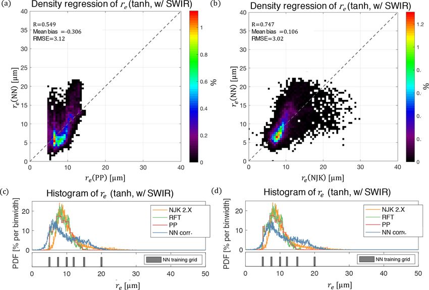
D. J. Miller et al.: Cloud property retrievals during ORACLES using a polarimetric neural network                                3451

gional differences in the cloud properties observed through-
out the campaign. Walvis Bay is located close to the climato-
logical center of the stratocumulus deck during the biomass
burning season, whereas flights out of São Tomé in 2017 (and
also in 2018) typically had to fly further south before en-
countering the stratocumulus cloud deck. As a consequence,
from an environmental perspective, the clouds observed dur-
ing the ORACLES 2016 field campaign were largely over-
cast marine stratocumulus but flights during 2017 observed
less homogeneous marine boundary layer clouds associated
with the transition between stratocumulus and broken cumu-
lus cloud regimes. In addition to the regional differences, the
behavior in the SE Atlantic changes to a greater extent sea-
sonally and to a lesser extent interannually. Seasonally, the
stratocumulus deck in this region shifts southward later in
the season with the cloud fraction maximum occurring in
September (Wood, 2012). In an interannual sense, the stra-
tocumulus deck is modified by changes in lower tropospheric
stability (LTS) that can be strongly correlated with sea sur-
face temperature and free tropospheric temperature (Wood,
2012). Because the ORACLES campaign spanned multiple
years and different seasons, the role of interannual variabil-
ity is important to consider. However, for the purposes of this
study, all of the variabilities result in greater diversity in the
cloud retrieval dataset, which we can use to gain a better un-       Figure 1. Flight tracks and study regions for the ORACLES 2016
derstanding of the behavior of our retrieval approach under          (dotted lines) and 2017 (dashed lines) field campaigns. Addition-
                                                                     ally, key take-off and landing locations are indicated and labeled
a variety of cloudy conditions.
                                                                     with green circles. Map data based on the Blue Marble: Next Gen-
    From an instrument perspective, the RSP flew on board            eration from the NASA Earth Observatory.
different flight platforms during the 2016 and 2017 deploy-
ments. In 2016, the NASA high-altitude ER-2 was dedicated
to remote sensing instruments, obtaining data from a near-
consistent flight altitude above 18 km. On the other hand, dur-      cool the detectors during some of the flights. As a conse-
ing 2017 (and 2018) the RSP flew on board the NASA P-3 at            quence, much of the 2017 dataset lacks data from the SWIR
a more variable range of altitudes, because the P-3 sampled          channels. To explore the consequence of the loss of the SWIR
throughout the boundary layer, in the cloud, in the aerosol          channels on our retrievals, we created two different training
layer, and above the cloud. As a consequence, the NN train-          datasets for our ORACLES 2017 NN retrieval scheme: one
ing sets for these 2 years differ from one another in order to       excluding the SWIR channels (applied on the entire dataset)
be appropriately tailored to the airborne platform differences,      and one that included the SWIR channels during training (ap-
mainly due to their different altitudes and the Rayleigh scat-       plied on the flights that acquired data with these channels).
tering differences. The training set for ORACLES 2016 was               Before performing the comparison of different retrieval
created for a constant aircraft altitude of 20 km, whereas the       methods, presented in Sect. 4, RSP data are first screened for
training set for ORACLES 2017 was constructed to account             a number of conditions to obtain useful comparable retrieval
for level legs at different aircraft altitudes. The differences      datasets. The philosophy behind this screening process is to
in the training set definition for each of these two datasets        obtain the best data for usage in this study but at the same
is further discussed in Sect. 3.1. Note that while ORACLES           time not cast aside NN retrievals that may be useful in future
2018 data are now available, they had not been available un-         studies. In addition to RSP data, we also use cloud-top height
til after the analysis of the this NN implementation was com-        data from the NASA Langley airborne second-generation
plete. However, the 2018 NN results will also be available in        high spectral resolution lidar (HSRL-2) to remove observa-
our data archive when they are completed. (Refer to the Data         tions of high-level or multilayer clouds in an attempt to limit
availability section for a link to the data archive.)                the retrieval to low-level marine boundary layer clouds (Hair
    As with any field campaign, instrument-specific compli-          et al., 2008; Burton et al., 2018). To that end, the following
cations arose that need to be considered. For example, the           screening criteria are applied to the datasets compared:
SWIR detectors of RSP must be cooled to obtain SWIR
reflectances without significant noise; however, during the            – cloudy scenes as identified by other RSP retrieval meth-
2017 field campaign there was a lack of liquid nitrogen to               ods,

https://doi.org/10.5194/amt-13-3447-2020                                               Atmos. Meas. Tech., 13, 3447–3470, 2020
3452                   D. J. Miller et al.: Cloud property retrievals during ORACLES using a polarimetric neural network

  – successful RSP retrievals using all other techniques,           data of different types (i.e., total or polarized reflected light),
                                                                    capability of retrieving different combinations of variables
  – coincident RSP and HSRL-2 data for cloud-top height             (i.e., some combination of re , ve , and τ ), and sensitivities
    definition, and                                                 (i.e., to cloud vertical profile, aerosol above cloud, or micro-
                                                                    physical regime).
  – instances with HSRL-2 cloud-top height below 2 km.
                                                                       The first method, often referred to as the bispectral
In a few limited cases coincident HSRL-2 and RSP data were          Nakajima–King (NJK) method, is an approach that takes
not available, which precludes some retrieval data from the         advantage of a difference in sensitivity to cloud optical
screening criteria above. The HSRL-2 screening criteria were        thickness and effective radius in a pair of spectral total re-
removed in the final data product (refer to the Data avail-         flectance bands (Nakajima and King, 1990). One band is
ability section) so that it could include NN retrievals for the     in a scattering-dominated visible-to-near-infrared (VNIR)
entire RSP dataset. Also included with the dataset is a guide       band, while the other is in a more absorptive shortwave in-
discussing how to evaluate the screening flags and select data      frared (SWIR) band. The NJK retrieval performed by RSP
suitable for other uses.                                            makes use of nadir-viewing total reflectances in the 0.865 µm
                                                                    and the 2.26 µm or 1.59 µm spectral bands. For the purposes
2.3    Standard RSP cloud retrievals                                of this study, we focus on the RSP NJK retrieval using the
                                                                    0.865 and 2.26 µm spectral band combination. This retrieval,
The shortwave radiative impact of clouds largely depends on         most notably implemented for the MODIS cloud retrieval
microphysical-scale cloud properties that define the droplet        product, is typically performed as a two-dimensional inter-
size distribution (DSD) (Twomey, 1977). Additionally, the           polation of observed reflectances within a discrete look-up
DSD also plays an important role in cloud-precipitation pro-        table (LUT), relating reflectances to unique pairs of re and
cesses (Pruppacher and Klett, 1978). In cloud remote sensing        τ values (Platnick et al., 2016). This particular method is
it is common to describe the cloud droplet size distribution        also important because it obtains a retrieval of cloud optical
using the gamma distribution presented in Hansen and Travis         thickness, while the following two methods, which are based
(1974), because it is both mathematically convenient and fits       on polarized reflectances, retrieve only droplet size distribu-
well to in situ observations (Deirmendjian, 1964; Tampieri          tion information (re , and ve ). As a consequence, these other
and Tomasi, 1976):                                                  methods secondarily perform an optical thickness retrieval in
                                                                  a manner similar to the NJK retrieval but with a single VNIR
                                   r                                band LUT with a preconstrained re obtained via a polarimet-
N(r) = N0 Cr (1−3ve )/ve exp −           ,               (6)
                                 re ve                              ric retrieval. In the context of the ORACLES field campaign
                                            −1                   it is also important to emphasize that the NJK method has
    C ≡ (re ve )(1−2ve )/ve 0 (1 − 2ve ) /ve

                                                  .      (7)
                                                                    been shown to be systematically biased by the presence of
                                                                    ACA – resulting in a high bias in both re and τ retrievals
This is a three-parameter distribution characterized by
                                                                    that is highly dependent on aerosol model assumptions, espe-
a droplet number concentration (N0 , cm−3 ), a droplet effec-
                                                                    cially those that can impact absorption (e.g., aerosol single-
tive radius (re , µm), and a droplet effective variance (ve , −).
                                                                    scattering albedo or refractive index) (Meyer et al., 2013).
The normalization constant for this distribution, C, is cal-
                                                                       The second RSP retrieval, referred to here as the para-
culated based on these parameters and the gamma function
                                                                    metric polarimetric method (PP), makes use of a library of
(0). The effective radius is a cross-section weighted droplet
                                                                    calculations that describe the angular distribution of single-
size that, for the purposes of light scattering applications,
                                                                    scattered polarized light (known as polarized phase functions
is usefully related to the scattering droplet size described in
                                                                    −P12 ). The phase functions and reflectances are both char-
Hansen and Travis (1974). The effective variance is related
                                                                    acterized by angular rainbow features (appearing between
to the droplet size distribution dispersion and can also be in-
                                                                    scattering angles of 130 and 170◦ ) that predictably shift and
terpreted as a measure of the asymmetry of the droplet size
                                                                    erode depending on the properties of the particular droplet
distribution.
                                                                    size distribution (i.e., the re and ve pair) (Bréon and Goloub,
       r3                                                           1998). Because polarized reflectances are dominated by sin-
re =        ,                                                (8)    gle scattering, this library can be used to obtain a best fit
       r2
                                                                    solution that matches the observed multiangular RP or DoLP
        1 (r − re )2 r 2                                            in a single spectral band. The phase function is then modi-
ve =                     .                                   (9)
       re2    r2                                                    fied by parametric functions that account for Rayleigh scat-
                                                                    tering and multiple scattering effects. The best fit solution
   The existing RSP liquid cloud retrieval products include         of this parametric phase function to the observed multian-
three very different methods of inferring cloud microphysical       gular reflectance corresponds to the droplet size distribution
information. Each of these methods differs from one another         parameters retrieved (Alexandrov et al., 2012a). The PP re-
in fundamental ways that include integrating observational          trieval can be performed for a number of different spectral

Atmos. Meas. Tech., 13, 3447–3470, 2020                                               https://doi.org/10.5194/amt-13-3447-2020
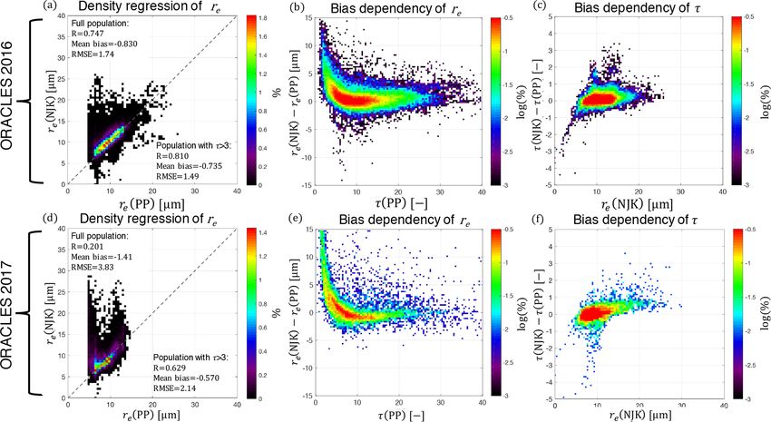
D. J. Miller et al.: Cloud property retrievals during ORACLES using a polarimetric neural network                              3453

bands, however, in this study we make use of the retrieval          the ORACLES 2016 comparison, it is evident that the two re-
performed for the 0.865 µm band. This is because the longer         trievals are similar to one another – with a correlation of R =
shortwave spectral bands have been shown to be more sen-            0.747, a mean bias of −0.830 µm, and a RMSE = 1.74 µm.
sitive to a greater range of droplet sizes at a fixed angular       It is noteworthy that despite being similar overall, the RMSE
resolution (Miller et al., 2018).                                   of the retrieval comparison is actually still quite large with
   The third RSP retrieval method is a non-parametric ap-           Fig. 2b, indicating that the re retrieval bias is being driven by
proach, known as the rainbow Fourier transform (RFT), that          retrievals of the low τ population (τ < 3). With that in mind,
retrieves the droplet size distribution in a functional form        the statistics for comparisons of the two retrievals excluding
via a mathematical transformation mapping the polarized re-         the low τ population are significantly improved. The com-
flectance in angular space to the droplet size distribution in      parison for ORACLES 2017 is more complicated, with in-
microphysical space. As the name indicates, this approach is        creased relative occurrence of thin clouds and increased spa-
similar to the relationship between oscillatory signals (fre-       tial inhomogeneity, the statistical metrics are much poorer –
quency space) and their corresponding Fourier transforms            with a correlation of R = 0.201, a mean bias of −1.41 µm,
(amplitude space) (Alexandrov et al., 2012b). This method           and a RMSE = 3.38 µm. However, this behavior is still, to
is useful for evaluating the assumption that droplet size dis-      a large extent, associated with the low τ population with
tributions are well behaved and mono-modal – an implicit            statistics improving when that population is excluded (look-
assumption for both of the gamma-distribution parameter re-         ing only at τ > 3) as indicated in Fig. 2. For both ORACLES
trievals discussed previously (Alexandrov et al., 2016). The        2016 (Fig. 2c) and ORACLES 2017 (Fig. 2f) datasets, the
RFT retrieval reports the distribution shape, but it also re-       comparison of τ reveals that there is typically very little rel-
ports the best-fit gamma-distribution parameters of the two         ative bias. In some cases, there are biases observed between
most prominent modes of the size distribution, resulting in re      the two retrievals corresponding to small NJK re retrievals
and ve retrievals for each mode. When we discuss the RFT            – indicating that using the PP constrained re retrieval pro-
retrieval in this study as a single re or ve value, we are always   duced a different τ retrieval. Given the statistical properties
referring to the most prominent mode of the size distribution.      of the comparisons of these two well-established retrieval ap-
   The physical differences between NJK and PP cloud prop-          proaches, we should expect to be satisfied if we find a similar
erty retrievals was recently the topic of research in Miller        degree of agreement between the NN retrieval and any of the
et al. (2018). One of the findings of that study was that high      standard RSP retrievals.
spatial resolution retrievals (50 m) mostly agreed with one
another to within the measurement uncertainties of the two
methods. However, at coarse spatial resolutions (> 300 m)           3     Neural network development
observations of spatially inhomogeneous cloud fields caused
the NJK retrieval to be biased high, resulting in differences       As discussed in Sect. 1, the NN architecture implemented in
between the two retrieval approaches. In the context of this        this study has changed significantly in response to the find-
study, airborne observations made by RSP have quite a high          ings of our previous work (Segal-Rozenhaimer et al., 2018).
spatial resolution (on the order of tens of meters to hun-          In Sect. 3.1 we will discuss the definition of the training set
dreds of meters, depending on aircraft altitude), which should      and particularities to the first 2 years of the ORACLES field
avoid some spatial inhomogeneity issues in this comparison.         campaign. Then, Sect. 3.2 discusses our new approach to pre-
Another finding by Miller et al. (2018) was that there can          processing input observations and uncertainties of total and
be significant high biases for the NJK retrieval when droplet       polarized reflectances. Finally, in Sect. 3.3 we outline the ar-
sizes become small (re ≈ 5 µm) or for optically thin clouds         chitectural variables such as network structure, learning rate,
(τ < 3). Given the high spatial and angular resolution of the       etc.
RSP retrievals in this study, it is likely that biases associated
with the “small and thin” population will be the most preva-        3.1    Training set simulations
lent source of bias in our data.
   In this study we intend to make informed comparisons be-         The synthetic observational dataset used to train the NN is
tween these already existing retrievals and the NN retrieval.       created using a vectorized radiative transfer (RT) model to
However, before doing that it is important to evaluate how          generate total and polarized reflectances that mimic the con-
these disparate retrieval products compare to one another. To       ditions of the observations made by the RSP instrument dur-
that end, Fig. 2 evaluates each of the retrievals against one       ing the ORACLES field campaign. The RT model used in this
another in much the same manner as in Miller et al. (2018).         study is the plane-parallel (1-D) polarized doubling–adding
All of these comparisons are made using ORACLES data that           (PDA) model developed at the NASA Goddard Institute for
have been previously screened for multilayer clouds, as de-         Space Studies. This model is built upon the methods de-
tailed in Sect. 2.2. The comparison of NJK and PP retrievals        scribed in van de Hulst and Irvine (1963) and can efficiently
of re are shown as density regressions for the ORACLES              solve radiative transfer problems in optically thick atmo-
2016 (Fig. 2a) and ORACLES 2017 (Fig. 2d) datasets. From            spheres (Hovenier, 1971; Hansen, 1971; Hansen and Travis,

https://doi.org/10.5194/amt-13-3447-2020                                              Atmos. Meas. Tech., 13, 3447–3470, 2020
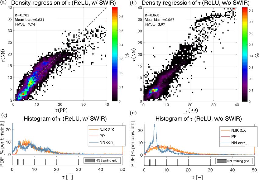
3454                  D. J. Miller et al.: Cloud property retrievals during ORACLES using a polarimetric neural network

Figure 2. A series of comparisons between the PP (using the 0.865 µm polarized reflectances) and NJK retrievals (using the 2.26 µm SWIR
band) made by RSP during ORACLES 2016 (a–c) and 2017 (d–f). In panels (a, d) NJK re (y axis) and PP re (x axis) retrievals are compared
using a density regression plot with a color bar that indicates the percentage of observations contained in each bin and a dashed one-to-one
line. In panels (a, b) the correlation, mean bias, and RMSE are reported for the full retrieval population, while the same statistics are also
reported for thick clouds (τ > 3) only in (c). Panels (d–f) use a different color bar that emphasizes features of smaller populations using the
logarithm of the percentage of observations in each bin. In panels (b, e) we display the bias between NJK and PP retrieval of re (y axis) is
shown with respect to the PP retrieval of τ (x axis). Finally, in panels (c, f) the bias between NJK and PP retrievals of τ (y axis) is shown
with respect to the NJK re retrieval.

1974; De Haan et al., 1987). This PDA radiative transfer                  paigns. Also, since the ER-2 is a high-altitude platform that
code was also selected to be used for inversions during the               flies at a constant altitude, the training set simulations (Ta-
Glory mission and therefore was specifically improved and                 ble 1) were made for a constant aircraft altitude of 20 km.
tailored for polarimetric accuracy (Cairns and Chowdhary,                 However, since the P-3 is a low-altitude flying platform, al-
2003). As a consequence, it is very efficient at generating the           titude variations were much larger than the ER-2, and the
simulated multispectral, multiangular polarimetric observa-               training set was constructed to predict measurements ob-
tions required to mimic the observations of the RSP instru-               tained along constant level legs of various altitudes (Table 2).
ment.                                                                     Additionally, there was slightly more variability in cloud-
   The training sets for the operational NN were generated                top height during 2017 as the clouds observed were often
based on the range of cloud properties observed in ORA-                   transitioning between low-level stratocumulus regime into
CLES 2016 (from RSP and in situ cloud measurements) and                   mid-level cloud regimes. Since the atmospheric scattering
were tailored for each of the airborne platforms, as discussed            between the flying platform and the cloud top has an effect
in Sect. 2.2. Compared to our training set generated in the               on the measured signals, the generated cases might not be
Segal-Rozenhaimer et al. (2018) study, these training sets ex-            optimal for all the scenes flown during 2017. This is a rela-
pand the relative azimuth angle (RAA) range significantly                 tively simplistic approach and certainly does not capture the
(from [0 : 10◦ ] to [0 : 90◦ ]) as shown in Table 1. This new             full variability of the observed data; as a result, the training
RAA range covers all possible azimuth geometries, since ra-               set simplifies some aspects of nature. For example, this ap-
diative transfer is symmetric about the solar plane and be-               proach would neglect the Rayleigh shielding effect, where an
cause the RSP scans in both forward and aft directions.                   increased cloud-top height would exclude more of the lower
   For all training sets, cloud-top height was fixed at 1 km,             atmosphere and therefore it’s contribution to the Rayleigh
which was found to be a reasonable assumption based on                    scattering signal from observed reflectances.
other independent measurements during the ORACLES cam-

Atmos. Meas. Tech., 13, 3447–3470, 2020                                                      https://doi.org/10.5194/amt-13-3447-2020
D. J. Miller et al.: Cloud property retrievals during ORACLES using a polarimetric neural network                                  3455

   Compared to the predecessor paper Segal-Rozenhaimer              input state vector by the variability in the dataset such that all
et al. (2018), we used a larger set of geometries and wider         inputs are constrained within a range in the following man-
range of parameter values but many of the same approx-              ner,
imations. For example, this training set assumes plane-                   xi − x
parallel radiative transfer (neglecting 3-D radiative effects)      xˆi =        ,                                             (10)
                                                                             s
and a “black” ocean surface with no reflections due to sun
glint or ocean color. The former is beyond our computing re-        where x is the mean of all x over all elements i, and s is
sources and desired level of parameterization, while the im-        the associated standard deviation. In contrast to this, we have
pact of the latter is expected to be heavily attenuated by the      modified this process so that measurement uncertainty is in-
cloud. It should also be noted that, as a matter of practice, we    corporated into the standardized data, such that the standard
attempted to keep the size of the training set used in this study   deviation is replaced by the expected measurement uncer-
reasonable to leave open the possibility of massively expand-       tainty of the mean observation obtained for the same geome-
ing the training data to include a large number of other inde-      try and band x (θ0 , θ, 1φ, λ),
pendent variables describing above-cloud aerosol properties                                 xi (θ0 , θ, 1φ, λ) − x (θ0 , θ, 1φ, λ)
                                                                    xˆi (θ0 , θ, 1φ, λ) =                                          , (11)
for use in future projects. The consequences and limitations                                          σ (x (θ0 , θ, 1φ, λ))
of using this limited training dataset and the role that other      where the measurement uncertainty, σ , is calculated using
training set decisions play in the behavior of our retrieval re-    the RSP uncertainty model in Knobelspiesse et al. (2019). We
sults will be discussed in Sects. 4 and 5.                          have explicitly noted the dimensions over which the average
                                                                    is calculated (solar zenith angle, view zenith angle, relative
3.2   Preprocessing input observations                              solar-view azimuth angle, spectral band [θ0 , θ , 1φ, λ]), such
                                                                    that a new standardization is calculated for the population
In our former NN retrieval scheme, we reduced the dimen-            of all training set data with the same geometry and wave-
sionality of the input layer by reducing measurement vec-           length. Both the training set and the observations go through
tor inputs to principal components (PCs) before introduc-           this preprocessing standardization process. After this stan-
ing them as input to the NN (Segal-Rozenhaimer et al.,              dardization relative to instrument uncertainty, the range of
2018). Our improved retrieval scheme described here is in-          variability in the DoLP training set input was approximately
stead trained with and applied to the measurement vector it-        4 times greater than the range of variability in the RI . As a re-
self. This solution was conceived to allow for more appro-          sult the network initially places greater weight on changes in
priate weighting of RI or DoLP, which have significantly            DoLP than on changes in RI . It is also important to note here
different measurement uncertainties. The size of the input          that after this initial preprocessing step, we also perform fur-
layer changed from 122 inputs (100 PC for DoLP, 20 for RI ,         ther input regularization and normalization as described in
and the two geometry inputs, i.e., SZA and RAA for each             the following section to help the network converge quickly
case) to 1570 (concatenating RI and DoLP, each spanning             during training.
784 values, covering the 112 instrument viewing angles in
seven wavelengths plus the two geometry input values). To           3.3     Neural network architecture and training
accommodate this 10-fold increase in the size of the input
layer, we implemented a new approach to our NN architec-            To handle the order-of-magnitude increase in the new input
ture, which will be discussed in Sect. 3.3. The advantage of        layer, we have been pushed to develop a deeper network ar-
this approach is that it allows us to adequately scale (weight)     chitecture. The new network, shown in Fig. 3, consists of
the different input sources (RI and DoLP) according to their        four subsequent hidden layers, each with 1024 nodes. This
measurement uncertainty. This is specifically important for         deep architecture contains more parameters that need to be
polarimetric observations, because both the magnitude and           trained, and as a consequence our approach to training has
uncertainty of RSP observations of RI and DoLP differ by an         also changed. In our previous work, we used a pure stochas-
order of magnitude. The uncertainty in RI is δRI ≈ 3 % and          tic back-propagation method that updated the weights in the
is largely dominated by systematic calibration-dependent bi-        hidden layer after each training sample. This network is in-
ases, whereas the uncertainty in DoLP is δDoLP ≈ 0.2 % and          stead trained using a mini-batch method, where a batch of
is largely dominated by random noise that varies with scene         samples (128) is presented to the network and the hidden
reflectance (RI ). Without consideration of the relative magni-     layer weights are only updated after each batch has been
tude and uncertainty, a NN incorporating both of these types        processed. In this architecture, following each hidden layer,
of observations would erroneously rely too much on high-            there is a batch normalization (BN) layer applied to the out-
magnitude and uncertainty RI observations at the expense of         puts of the layer. The purpose of the BN layer is to increase
low-magnitude and uncertainty DoLP. To avoid this issue,            the stability of the neural network, by subtracting the batch
we incorporate knowledge of measurement uncertainty into            mean and dividing by the batch standard deviation. By ap-
a vector standardization process that is applied prior to NN        plying this transformation, it keeps the inputs into the subse-
training and application. Typically, standardization scales the     quent activation layer stable (not too high and not too low),

https://doi.org/10.5194/amt-13-3447-2020                                               Atmos. Meas. Tech., 13, 3447–3470, 2020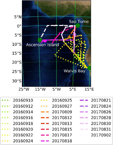
3456                 D. J. Miller et al.: Cloud property retrievals during ORACLES using a polarimetric neural network

Table 1. Parameter grid space used to generate the training set for the operational NN used for cloud retrievals from the ER-2 during
the ORACLES 2016 field campaign. This contains N = 44 064 feature vectors, with each vector containing N ≈ 1600 labeled datapoints
corresponding to radiometric variables (I and DoLP), wavelengths, across all VZAs. Aircraft altitude is set as constant at 20 km, and cloud
top altitude was also fixed at 1 km.

                    Parameter (units)    No. of grid points   Training grid
                    re (µm)                              6    5, 7.5, 10, 12.5, 15, 20
                    ve (–)                               6    0.01, 0.03, 0.05, 0.07, 0.1, 0.15
                    τ (–)                                6    2.5, 5, 10, 15, 20, 30
                    SZA (◦ )                            12    10, 15, 20, 25, 30, 35, 40, 45, 50, 55, 60, 65
                    RAA (–)                             17    0, 2, 4, 6, 8, 12, 16, 20, 24, 28, 32, 40, 50, 60, 70, 80, 90

Table 2. Parameter grid space used to generate the training set for the operational NN used for cloud retrievals from the P-3 during the
ORACLES 2017 field campaign. This contains N = 261 144 feature vectors, with each vector containing N ≈ 1600 labeled datapoints
corresponding to radiometric variables (I and DoLP), wavelengths, across all VZAs.

                               Parameter (units)       No. of grid points     Training grid
                               Aircraft altitude (m)                   3      5000, 6000, 7000
                               re (µm)                                 6      5, 7.5, 10, 12.5, 15, 20
                               ve (–)                                  6      0.01, 0.03, 0.05, 0.07, 0.1, 0.15
                               τ (–)                                   6      2.5, 5, 10, 15, 20, 30
                               SZA (◦ )                               13      5 to 65 in increments of 5
                               RAA (◦ )                               31      0 to 90 in increments of 3

maintaining the mean activation close to 0 and the activa-
tion standard deviation close to 1, to help with the network
training convergence. In the activation layer, we make use of
either a hyperbolic tangent (tanh(θ )) or rectified linear unit
function (ReLU(θ )), the latter of which is zero for all neg-
ative inputs and linearly increases for positive inputs. The
tanh activation is widely used as the standard in NN litera-
ture (e.g., LeCun et al., 1989, 1998), while ReLU is gaining
more popularity recently due to its simplicity and its ability
to greatly accelerate the convergence of stochastic gradient
descent (SGD) algorithms and their variations (Krizhevsky               Figure 3. Architecture of the operational NN scheme used for the
et al., 2012). In Segal-Rozenhaimer et al. (2018), we did not           retrieval of ORACLES 2016–2017 RSP measurements. The net-
notice a large difference between these two activation func-            work contains four subsequent hidden layers, as detailed in the text.
tions, but for this larger NN, we find differences in retrieval
performance that we will discuss in detail in Sect. 4. Finally,
the output layer activation function is linear, with a loss func-
tion defined as the mean-square error (MSE) and results in              (SGD) optimization algorithm, Adam is computationally ef-
the predicted values of τ , re , and ve .                               ficient, has little memory requirements, and is well suited for
   During the training process, the input vector, which has al-         problems that are large in terms of data and/or parameters
ready been preprocessed as detailed in the former section, is           (Kingma and Ba, 2014). The network is trained with a learn-
further linearly scaled to have values between −1 and 1. This           ing rate of 0.0001 using the “mini-batch” method to complete
is performed to allow for better convergence during train-              an epoch, while the number of epochs per training scenario
ing. Also, the training process is being regularized by adding          was 100. Following training, the network was evaluated us-
Gaussian noise to the input layer during the training phase.            ing an evaluation dataset consisting of a subset of training set
The optimization algorithm used here is Adam (Adaptive                  data that were set aside during the training phase. Taking the
moment estimation), implemented within the Keras python                 network trained for ORACLES 2016 using tanh activation as
API (Chollet, 2017) with a TensorFlow back end (a sys-                  an example, comparison with the evaluation dataset resulted
tem for large-scale machine learning) (Abadi et al., 2016).             in correlations of 0.999, 0.987, and 0.941; absolute biases of
In comparison with the classic stochastic gradient descent              0.016, 0.044 µm, and 0.094; and RMSEs of 0.021, 0.076 µm,
                                                                        and 0.16 each for τ , re , and ve , respectively. The results for

Atmos. Meas. Tech., 13, 3447–3470, 2020                                                       https://doi.org/10.5194/amt-13-3447-2020
D. J. Miller et al.: Cloud property retrievals during ORACLES using a polarimetric neural network 3457
τ and re are quite promising, but the RMSE in the ve evalu- that the NN retrieval is otherwise generally performing cor-
ation after training is enough to span the possible state space rectly. In particular, we expect that this bias is an expression
– an indication that this network cannot adequately retrieve of a difference between the assumptions built into the net-
ve . It is important to note that other neural network studies work training dataset that differ from the observation dataset.
have demonstrated better retrieval quality for ve with differ- We will discuss the possible sources of these differences in
ent input and architecture decisions (Di Noia et al., 2019). We Sect. 5.
also compared ve (N N ) to RSP retrievals and found signifi- Given the high correlations, linearity of the initial output,
cant variability and large biases that were inconsistent with and results from the network training evaluation, we believe
both studies of RSP retrieval sensitivity (Alexandrov et al., the linear offsets of these regressions are artifacts. To cor-
2012a), as well as other studies focused on similar polarime- rect the persistent linear offset of the NN retrievals, we apply
ter retrievals (Shang et al., 2019). a linear scaling to them by creating what we refer to as our
adjusted NN retrieval product. Ideally and in principle this
could be done with a small validation dataset that is not re-
4 Results lated to the retrieval products we hope to later compare our
results to. Without an external dataset to scale to, we have de-
4.1 Initial output and postprocessing cided to linearly scale the NN retrievals to a subset of 10 % of
the total population of RSP data (in this example for the OR-
The output from the network initially reveals some issues that ACLES 2016 dataset). This avoids explicitly fitting all NN
still need to be addressed. Our approach to evaluating the be- retrievals via fitting. This dataset is then regressed against
havior of the output layer results is to explore comparisons the corresponding τ (PP) and re (PP) retrievals to obtain two
to the RSP retrievals. Throughout the following we will re- linear correction terms, the offset bias (b) and the scaling bias
fer to network output layer results as the “initial output” to (m),
indicate that it has not undergone any postprocessing. As in-
dicated in Sect. 2.3, we are particularly interested in the RSP xNN = mxPP + b, (12)
PP retrieval comparison as this provides the most consistent 1
x̂NN = (xPP − b) , (13)
retrieval results in conditions with varying cloud inhomo- m
geneity and in the presence of above-cloud aerosols. Overall, where x̂NN corresponds to a linearly adjusted neural network
this comparison revealed correlations for the re retrievals are retrieval output, m is the scale correction, and b is the linear
lower (R ≈ 0.7) than for the τ (R ≈ 0.9) retrieval irrespec- offset correction. After the components of this linear adjust-
tive of the network activation function used. An interesting ment are determined using the subset of PP retrievals, the
finding of this initial analysis was that networks using differ- NN retrievals are adjusted (i.e., the x̂NN product is created).
ent activation functions produced different behaviors for the Finally, this adjusted NN retrieval product can be compared
retrievals of τ than they did for re . This is demonstrated in to the other retrievals using the full RSP dataset – including
Table 3 using the ORACLES 2016 network and data, where the portion that was excluded from this correction definition
the correlations for re retrievals improve for networks using exercise. The application of this linear correction does not
a tanh activation function, while in contrast τ retrievals have influence the correlation of the retrievals; however, it does
improved correlations for networks using a ReLU activation result in lower mean and RMSE biases for this ORACLES
function. This behavior is a symptom of a feature we ob- 2016 example shown in Fig. 4. For re , the mean bias is re-
served rather than being linearly related to the PP retrieval duced to 0.023 µm and the RMSE is 1.74 µm, whereas for
of τ ; the tanh-based τ retrieval demonstrated a nonlinear or τ the mean bias is −0.050 and the RMSE is 1.82. Further
logarithmic dependence with increasing τ . A similar behav- discussions of the behavior of the adjusted NN datasets are
ior was exhibited for the PP retrieval of re and the ReLU- separated into Sect. 4.2 and 4.3, where each discusses and
based re retrieval. As a consequence, throughout the rest of highlights behaviors of the NN retrieval for the ORACLES
this study, we will perform retrievals for re and τ with two 2016 and 2017 datasets, respectively.
different networks: for re we make use of the tanh network
and for τ we make use of the ReLU network. This approach 4.2 Results for ORACLES 2016
will be further discussed in Sect. 4.2.
Beyond simply evaluating correlations, the raw output of From a number of perspectives, the ORACLES 2016 cam-
the network exhibits clear linear offsets when compared to paign data are easy to work with: RSP was flying on a ded-
the other RSP retrievals. In particular we emphasize this be- icated remote sensing platform (NASA high-altitude ER-
havior for the PP retrievals in Fig. 4. This linear bias was 2), there were prevalent observations of clouds, and data
absent during our training set validation exercise in Sect. 3.3, availability was often not an issue. As a consequence, the
implying that this systematic offset is a consequence of dif- dataset analyzed here is large – including 6 d of flights with
ferences between training set and observational data. Despite N = 72 542 retrievals that pass all of the analysis filter crite-
this linear bias, the high correlations of these retrievals imply ria introduced in Sect. 2.2.
https://doi.org/10.5194/amt-13-3447-2020 Atmos. Meas. Tech., 13, 3447–3470, 2020You can also read