Very high stratospheric influence observed in the free troposphere over the northern Alps - just a local phenomenon?
←
→
Page content transcription
If your browser does not render page correctly, please read the page content below
Atmos. Chem. Phys., 20, 243–266, 2020
https://doi.org/10.5194/acp-20-243-2020
© Author(s) 2020. This work is distributed under
the Creative Commons Attribution 4.0 License.

Very high stratospheric influence observed in the free troposphere
over the northern Alps – just a local phenomenon?
Thomas Trickl1 , Hannes Vogelmann1 , Ludwig Ries2 , and Michael Sprenger3
1 Karlsruher Institut für Technologie, Institut für Meteorologie und Klimaforschung, IMK-IFU,
Kreuzeckbahnstr. 19, 82467 Garmisch-Partenkirchen, Germany
2 Umweltbundesamt II 4.5, Plattform Zugspitze, GAW-Globalobservatorium Zugspitze-Hohenpeißenberg,

Schneefernerhaus, 82475 Zugspitze, Germany
3 Eidgenössische Technische Hochschule (ETH) Zürich, Institut für Atmosphäre und Klima,

Universitätstraße 16, 8092 Zürich, Switzerland

Correspondence: Thomas Trickl (thomas.trickl@kit.edu, thomas@trickl.de)

Received: 19 June 2019 – Discussion started: 12 August 2019
Revised: 20 November 2019 – Accepted: 2 December 2019 – Published: 6 January 2020

Abstract. The atmospheric composition is strongly influ-         tion of ozone import from the stratosphere to tropospheric
enced by a change in atmospheric dynamics, which is po-          ozone.
tentially related to climate change. A prominent exam-
ple is the doubling of the stratospheric ozone component
at the Zugspitze summit station (2962 m a.s.l., Garmisch-
Partenkirchen, Germany) between the mid-seventies and
2005, roughly from 11 to 23 ppb (43 %). Systematic ef-           1   Introduction
forts for identifying and quantifying this influence have been
made since the late 1990s. Meanwhile, routine lidar measure-     For many years the pronounced rise of tropospheric ozone
ments of ozone and water vapour carried out at Garmisch-         due to growing anthropogenic air pollution has been the sub-
Partenkirchen (German Alps) since 2007, combined with in         ject of intensive research. The background level of ozone has
situ and radiosonde data and trajectory calculations, have re-   reached 50 ppb and more at some sites at the northern mid-
vealed that stratospheric intrusion layers are present on 84 %   latitudes (e.g. Parrish et al., 2012; Gaudel et al, 2018). How-
of the yearly measurement days. At Alpine summit stations        ever, megacity ozone may reach even several hundred ppb
the frequency of intrusions exhibits a seasonal cycle with a     (e.g. Parrish et al., 2011, 2016) that may ultimately contribute
pronounced summer minimum that is reproduced by the li-          to the tropospheric ozone background.
dar measurements. The summer minimum disappears if one              On the other hand, the most important natural source of
looks at the free troposphere as a whole. The mid- and upper-    tropospheric ozone, i.e. the import from the stratosphere, has
tropospheric intrusion layers seem to be dominated by very       been frequently related to the Montsouris value of just about
long descent on up to hemispheric scale in an altitude range     10 ppb estimated for the late 19th century (Volz and Kley,
starting at about 4.5 km a.s.l. Without interfering air flows,   1987). Layers of stratospheric air can be identified directly
these layers remain very dry, typically with RH ≤ 5 % at the     based on criteria like elevated ozone and low humidity. This
centre of the intrusion. Pronounced ozone maxima observed        direct import in deep stratospheric air intrusions has long re-
above Garmisch-Partenkirchen have been mostly related to a       sulted in estimates of the stratospheric influence on the tropo-
stratospheric origin rather than to long-range transport from    spheric ozone level of about 10 % and less (e.g. Elbern et al.,
remote boundary layers. Our findings and results for other       1997; Beekmann et al., 1997; Stohl et al., 2000). This would
latitudes seem to support the idea of a rather high contribu-    suggest a rather small relative importance of stratosphere-to-
                                                                 troposphere transport (STT), with some uncertainty originat-
                                                                 ing from the “indirect” stratospheric component that cannot

Published by Copernicus Publications on behalf of the European Geosciences Union.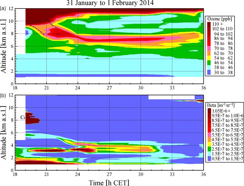
244                                                                          T. Trickl et al.: Very high stratospheric influence

be detected due to complete mixing of the stratospheric in-         layer structure in the free troposphere (Newell et al., 1998;
trusions into the troposphere.                                      Thouret et al., 2000). The layers were identified by positive
   Quantifying STT has been attempted for more than half a          or negative departures from the mean background. The layers
century. Whereas early studies aimed at identifying the STT         with excess ozone and reduced water vapour clearly domi-
mechanisms (e.g. Danielsen, 1968), more recent work has             nate, with about 50 % of the cases in all regions. Although the
also estimated the STT budget by extrapolations of observa-         threshold for relative humidity drops applied (5 %) is much
tional data (e.g. Danielsen and Mohnen, 1977; Viezee et al.,        lower than needed for verifying STT (Trickl et al., 2014,
1983; Beekmann et al., 1997) or by diagnosing the cross-            2015), this high fraction is a hint towards significant down-
tropopause transport by global and regional weather and             ward transport. The occurrence of dry layers with elevated
climate models (e.g. Roelofs and Lelieveld, 1997; Kentar-           ozone maximizes between 4 and 6 km.
chos and Roelofs, 2003; Stevenson et al., 2006; Wild, 2007;            The global distribution of tropopause folds is rather inho-
Young et al., 2013). Model-based approaches have frequently         mogeneous with maxima in regions around the jet streams
concentrated on the overall exchange rate (for STE) rather          (e.g. James et al., 2003; Sprenger et al., 2003; Škerlak et al.,
than on that for STT. In the most recent multi-model com-           2014)). Sprenger et al. (2003) found that the role of the sub-
parison (Young et al., 2013) the models agree within about          tropical jet stream (STJ) for STT had been strongly underes-
±20 % (standard deviation) around an average net STE rate           timated. The STJ persists during most of the year (Koch et
of 477 Tg a−1 . This value, obtained as a difference of the         al., 2006) and, thus, could be associated with frequent verti-
steady-state photochemical production rate and the loss rates,      cal exchange. However, it is not only the persistence that mat-
is just about 10 % of the production rate. The ozone mixing         ters: high ozone values have also been reported in subtropi-
ratio due to STT was e.g. obtained from semi-Lagrangian             cal intrusions. For example, very strong ozone signatures in
approaches such as by Roelofs and Lelieveld (1997) or               the troposphere exceeding 200 ppb have been detected over
Collins et al. (2003). Roelofs and Lelieveld (1997) found           northern India (Ojha et al., 2014, 2017). High ozone values
a fraction due to STT of 40 % in tropospheric ozone. This           in the middle and upper troposphere from regions next to the
value looks rather high given the coarse resolution of the          STJ have even been observed above Garmisch-Partenkirchen
underlying chemistry-transport model of (e.g. horizontally)         (Germany) after transport almost all the way around the
3.75◦ × 3.75◦ that is insufficient for resolving thin strato-       Northern Hemisphere (six cases: Trickl et al., 2011; see also
spheric layers in the troposphere (see Roelofs et al., 2003;        Langford, 1999). In general, observations at the source lat-
Rastigejev et al., 2010; Easthman and Jacobs, 2017). The            itudes have been limited (e.g. Gouget et al., 1996; Cammas
stratospheric contributions of Collins et al. (2003) are lower      et al., 1998; Kowol-Santen and Ancellet, 2000; Zachariasse,
(roughly 30 % above mid-latitude sites, the average mixing          2000; Zahn et al., 2002). Beyond the regions around the STJ,
ratio typically rising from 40 to 60 ppb from the lower to up-      STT has been found in the tropics. For example, during 30 %
per troposphere) and vary from site to site. In a study with        of the MOZAIC flights across the tropical Atlantic at least
higher spatial resolution, Jaeglé et al. (2017) examined STT        one event with more than 100 ppb of ozone occurred, which
in dry intrusions associated with extratropical cyclones. They      was associated with strong convection in the Inter-Tropical
found that, on average, 15 % of the ozone mass in a dry in-         Convergence Zone (Suhre et al., 1997).
trusion is irreversibly mixed into the troposphere.                    A great surprise was the detection of a substantial
   In principle, a quantification of STT should involve ob-         stratospheric influence at the Zugspitze mountain-top site
servations. However, determining the STT flux from obser-           (2962 m a.s.l.) in the German Alps and its pronounced pos-
vations is a highly demanding task. Assessments from ob-            itive trend (Fig. 1). In assessments of long-term ozone series
servations are easier for STT than for TST (troposphere-to-         the Zugspitze O3 exhibited the strongest increase (e.g. Par-
stratosphere transport) since both ozone and water vapour are       rish et al., 2012; Logan et al., 2012; Oltmans et al., 2012).
suitable complementary tracers. The results strongly depend         The Zugspitze ozone increased from 1978 to 2003, in con-
on the criteria selected for data filtering based on tracers such   trast to the neighbouring Wank site (1780 m a.s.l.), where the
as O3 , H2 O or 7 Be (e.g. Stohl et al., 2000). In addition, mix-   annual-average ozone level has remained constant since the
ing of the dry descending layers with tropospheric air must         1980s. We have explained (Trickl et al., 2010) the difference
be taken into account, which was, however, recently found           between Zugspitze and Wank ozone by a much larger amount
to be much less severe than previously thought (Trickl et al.,      of stratospheric air reaching the higher of the two summits
2014, 2016).                                                        (e.g. Elbern et al., 1997).
   Gradually, STT has turned out to be potentially much                The positive trend of stratospheric influence is seen in the
more important than concluded from the early assessments.           contributions of both the “direct” descent to the Zugspitze
For instance, a correlation study of O3 and H2 O based on           summit, characterized by distinct ozone and humidity struc-
vertical profiles derived from aircraft ascents and descents        tures, and the “indirect” contribution of aged stratospheric
in the vicinity of airports within the MOZAIC (Measure-             intrusions strongly mixed with the surrounding tropospheric
ment of Ozone, Water Vapour by Airbus In-Service Aircraft,          air (Fig. 1). The direct contribution (< 10 %) was obtained
Marenco et al., 1998) project revealed a rich (“ubiquitous”)        from correlating low humidity with elevated 7 Be (Scheel,

Atmos. Chem. Phys., 20, 243–266, 2020                                                 www.atmos-chem-phys.net/20/243/2020/
T. Trickl et al.: Very high stratospheric influence                                                                                  245

                                                                        sphere over Europe back to 1970 from the analysis of long-
                                                                        term ozonesonde data. Central Europe is located at the exit
                                                                        of the North Atlantic storm track and, therefore, is a receptor
                                                                        region for subsiding stratospheric layers. A possible explana-
                                                                        tion of the positive trend in our view could be a reaction of the
                                                                        atmospheric dynamics to climate change (see also Collins et
                                                                        al., 2003; Yang et al., 2016; Lin et al., 2015; Neu et al., 2014).
                                                                           Dibb et al. (2003) determined the latitudinal distribution
                                                                        of STT over North America by a total of 39 air-chemistry
                                                                        aircraft missions from Boulder (Colorado, USA, 40◦ N) to up
                                                                        to 86◦ N. The altitude varied between the surface and about
                                                                        7000 m. These flights were special since also here 7 Be filter
                                                                        samples were taken as an additional indicator of stratospheric
Figure 1. Annual mean ozone mixing ratios for the Zugspitze sum-        air, an advantage which is normally limited to surface sites.
mit from 1978 to 2003, together with preliminary estimates of the       Stratospheric influence was identified on 23 of the flights,
directly detected stratospheric component (red) and of the indi-        most of the intrusions being detected near and above 6 km.
rect component (blue) obtained from 7 Be measurements: the strato-      Above 6 km the flights took place in stratospheric air during
spheric influence doubled during that period. As a consequence af-      more than half of the time, indicating an extreme transfer of
ter 1981 the positive ozone trend disappears after subtracting the      ozone in that altitude range. Below 50◦ N the stratospheric
evaluated stratospheric fraction of ozone. The figure of H. E. Scheel   layers were limited to this altitude range.
is taken from the ATMOFAST final report (2005; Fig. 2.40 on
                                                                           The seasonal cycle of the stratospheric ozone contribu-
p. 67).
                                                                        tion at Alpine summit stations exhibits a pronounced sum-
                                                                        mer minimum (Elbern et al, 1997; Stohl et al., 2000; Trickl
                                                                        et al., 2010). In contrast to this, Beekmann et al. (1997) con-
2003, pp. 66–71 in ATMOFAST, 2005). Aged stratospheric                  cluded for the entire free troposphere above three European
air masses that are completely mixed into the troposphere               ozonesonde stations a seasonal cycle with a slight summer
cannot be identified by data filtering and, therefore, had not          maximum, based on data filtering of ozone profiles between
been derived in studies based on observations. In order to              1969 and 1994. A transition to this behaviour is indicated
obtain some guess of the indirect component of STT in the               for growing altitude of the Alpine stations: the summer min-
Zugspitze ozone, Scheel (in ATMOFAST, 2005) determined                  imum is least pronounced at the highest of the stations pre-
a 7 Be-to-ozone conversion factor from the direct component,            viously compared, Jungfraujoch (see Fig. 1 of Trickl et al.,
considering that 2/3 of 7 Be is produced in the stratosphere            2010).
(Lal and Peters, 1967). The results in Fig. 1 are associated               Motivated by all these findings, we extend in this paper
with an uncertainty of unknown magnitude, in part because               our STT studies to the full free troposphere. The analysis is
of the limited decay time of 7 Be (53.42 d (±0.01 d); Huh and           based on routine lidar measurements of ozone, water vapour
Liu, 2000). However, they are plausible since the 1978 strato-          and aerosol since 2007, as well as radiosonde relative hu-
spheric fraction of 11.3 ppb (31.2 %) is in the expected range          midity and transport modelling. The resulting stratospheric
of values derived from measurement in the late 19th century             component in tropospheric ozone over central Europe is sur-
(Volz and Kley, 1988; Marenco et al., 1994). From the de-               prisingly strong. We see some confirmation of our findings
cline of the ozone precursors over Europe in the 1990s (e.g.            in recent lidar and sonde results from lower latitudes which
Jonson et al., 2006; Vautard et al., 2006), one would expect a          will be discussed in detail in Sect. 4.
negative development. Thus, the estimate of the stratospheric              After introducing the observational methods and the mod-
component is perhaps even somewhat conservative (see Tara-              els used in Sect. 2, we describe the data selection approach
sick et al., 2019a, for a more thorough discussion of possibly          for STT events (Sect. 3.1). In Sects. 3.2 and 3.3 we give typ-
higher pre-industrial ozone levels).                                    ical examples for the most important intrusion types and dis-
   A comparable positive ozone trend is also reported for the           cuss the role of STT during the warm season in comparison
Swiss Jungfraujoch station (3580 m a.s.l.) where the ozone              with long-range transport of high ozone advected from re-
measurements started in 1992 (Ordoñez et al., 2007). For the            mote pollution events by intercontinental transport. Section 3
lower-lying Italian station Monte Cimone (2165 m a.s.l.), no            describes the details of the statistical analysis of the fraction
significant correlation between ozone and the intrusion fre-            of STT days 2007–2016. Finally, an overall discussion and
quency was detected. However, this conclusion is only based             conclusions are given in Sect. 4.
on the years 1996 to 2011, i.e. for a time period that is rather
late compared with the ozone rise at the Alpine sites (Cristo-
fanelli et al., 2015). Finally, Colette and Ancellet (2005) re-
trieved an increase in stratospheric ozone in the entire tropo-

www.atmos-chem-phys.net/20/243/2020/                                                        Atmos. Chem. Phys., 20, 243–266, 2020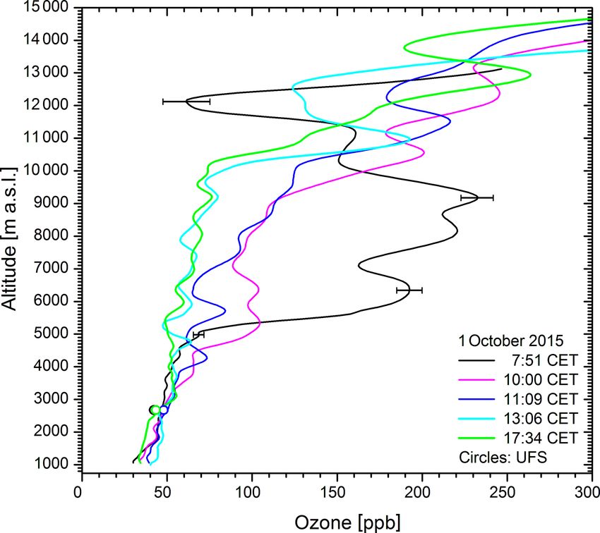
246                                                                          T. Trickl et al.: Very high stratospheric influence

2     Methods                                                          Aerosol backscatter profiles with a very good signal-to-
                                                                    noise ratio up to the lower stratosphere are obtained from
2.1     Measurements                                                the 313 nm “off” channel of the lidar. The methods, im-
                                                                    plying an ozone correction, have been described by Eisele
                                                                    and Trickl (2005). Examples demonstrating the data qual-
2.1.1    IFU ozone DIAL                                             ity achieved in recent years (maximum noise level of the
                                                                    backscatter coefficients ±1 × 10⁻⁷ m−1 sr−1 , reached in the
The tropospheric ozone lidar is operated in Garmisch-               tropopause region) can be seen in Trickl et al. (2015). We
Partenkirchen, Germany, at IMK-IFU (formerly IFU;                   derive vertical profiles of the aerosol backscatter coeffi-
47◦ 280 3700 N, 11◦ 30 5200 E; 740 m a.s.l.). The laser source is   cients based on a constant backscatter-to-extinction ratio of
a Raman-shifted KrF laser, and two separate receiving tele-         0.020 sr−1 , which is the average value derived within the
scopes are used to divide the dynamic range of the backscat-        European Aerosol Research Lidar Network (EARLINET,
ter signal of roughly 8 decades. This lidar was completed           2003). Within clouds larger values are taken, if possible op-
as a two-wavelength differential-absorption lidar (DIAL) in         timized for minimum discrepancy of the backscatter profiles
1990 (Kempfer et al., 1994) and a first annual sounding se-         below and above the cloud.
ries was achieved in 1991 (Carnuth et al., 2002). It was
upgraded to a three-wavelength DIAL in 1994 and 1995
                                                                    2.1.2   IFU water-vapour DIAL at the Schneefernerhaus
(Eisele and Trickl, 1997), leading to a unique vertical range
                                                                            high-altitude station
between roughly 0.25 km above the ground and 3 to 5 km
above the tropopause, the measurement time interval being
just 41 s. By comparing the ozone profiles retrieved from dif-      The Zugspitze water-vapour DIAL is operated at the
ferent wavelength combinations (e.g. 277–313 nm or 292–             Schneefernerhaus high-altitude research station (UFS,
313 nm), an internal quality check is possible. The choice of       47◦ 250 0000 N, 10◦ 580 4600 E) at 2675 m a.s.l., about 8.5 km to
an “on” wavelength below 280 nm is particularly beneficial          the south-west of IMK-IFU (Garmisch-Partenkirchen, Ger-
for achieving a high accuracy and a high vertical resolution        many), and 0.5 km to the south-west of the Zugspitze sum-
(up to about 5 km above the ground). Density has been con-          mit. The full details of this lidar system were described by
verted to mixing ratio by using pressure and temperature data       Vogelmann and Trickl (2008). It is based on a powerful tun-
from nearby radiosonde stations (Sect. 2.1.4).                      able narrow-band Ti : sapphire laser system with up to 250 mJ
   The noise level of the system since late 2012 is ±1 × 10⁻⁶       energy per pulse operated at about 817 nm and a 0.65-m-
of the input voltage range of the digitizer system. The DIAL        diameter Newtonian receiver. Due to these specifications a
features low uncertainties of about ±2 ppb in the lower free        vertical range up to about 12 km can be reached, almost un-
troposphere, approximately tripling (under optimum condi-           affected by daylight. However, mostly the laser has been op-
tions) in the upper troposphere because of the use of the           erated at half the maximum pulse energy or less to extend the
292–313 nm wavelength pair. Comparisons with the nearby             life time of the high-voltage components such as flashlamps.
Zugspitze in situ measurements (at 2962 m a.s.l.; see below)        A separation of near-field and far-field signals is achieved
show no relevant mutual bias, the standard deviation of the         by a combination of a beam splitter and a blade in the far-
differences being less than 2 ppb. The uncertainty further di-      field channel. The operating range starts below the altitude
minished after another system upgrade in 2012, after intro-         of the summit station (2962 m a.s.l.). The electronics are al-
ducing a new ground-free input stage to our transient digi-         most identical to those of the ozone DIAL. However, at the
tizers (Licel) that reduced the noise level by roughly a factor     operating wavelength of 817 nm avalanche photodiodes have
of 3. For the range covered by the near-field receiver (be-         been used that introduce higher noise than the photomulti-
low 1.2 km above the lidar), the uncertainty is of the order        plier tubes preferred for shorter wavelengths. Thus, the sys-
of ±5 ppb. The upper-tropospheric performance may be de-            tem has not yet reached its expected optimum performance
graded in the presence of high lower-tropospheric ozone con-        in the upper troposphere.
centrations absorbing a lot of the ultraviolet laser emission          The vertical resolution chosen in the data evaluation is
and by enhanced sky light in summer, in particular in the           dynamically varied between 50 m in altitude regions with
presence of clouds. The vertical resolution is dynamically          a good signal-to-noise ratio and roughly 350 m in the up-
varied between 50 m and a few hundred metres, depending             per troposphere. Free-tropospheric measurements during dry
on the signal-to-noise ratio decreasing with altitude. Within       conditions clearly benefit from the elevated site outside or
stratospheric intrusion layers the vertical smoothing is re-        just below the edge of the moist Alpine boundary layer (e.g.
duced as far as possible in order to avoid a reduction of the       Carnuth and Trickl, 2000; Nyeki et al., 2000; Carnuth et al.,
peak concentrations by smoothing. The lidar has been used           2002). After a few years of testing, validating and optimiz-
in numerous atmospheric transport studies (e.g. Eisele et al.,      ing the system, routine measurements started in January 2007
1999; Stohl and Trickl, 1999; Trickl et al., 2003; and other        with typically 2 measurement days per week, provided that
publications cited in this paper).                                  the weather conditions were favourable. Operation has been

Atmos. Chem. Phys., 20, 243–266, 2020                                                  www.atmos-chem-phys.net/20/243/2020/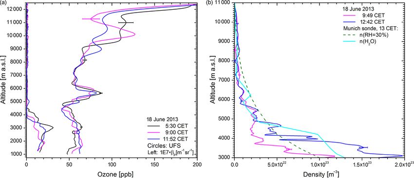
T. Trickl et al.: Very high stratospheric influence                                                                            247

interrupted since winter 2015 due to fatal laser damage. A          of ozone DIAL and UFS are highly satisfactory, with dif-
new Ti : sapphire laser system is under development.                ferences mostly staying below 2 ppb. However, orographic
   The lidar has been validated in several comparisons with         air-mass lifting must be taken into account that can lead to
local and remote radiosonde ascents (Vogelmann and Trickl,          vertical displacements of ozone structures and larger differ-
2008), an airborne DIAL (Trickl et al., 2016) and the               ences between lidar and in situ data.
Zugspitze Fourier transform spectrometer (Vogelmann et al.,
2011). A noise level of 5 % and a bias of 1 % at most was ver-      2.1.4    Sonde data
ified to altitudes of more than 6 km. Furthermore, a very high
importance of volume matching in comparisons of water-              Radiosonde data are routinely used for calculating the atmo-
vapour profiling instruments was found (Vogelmann et al.,           spheric density, which is necessary for quantitative aerosol
2011, 2015), on the scale of a quarter of an hour and a few         retrievals and the conversion of the ozone or the water-
kilometres.                                                         vapour number density to mixing ratio. Most importantly,
   In some cases, in which a direct comparison of the ex-           on each measurement day of the ozone DIAL the presence
act matching of the humidity and aerosol layers was neces-          of dry and moist layers was examined in order to identify
sary (e.g. Trickl et al., 2016), aerosol backscatter coefficients   potential advection from a remote stratosphere or (marine)
were retrieved from the “off” wavelength channel. The cal-          boundary layer, respectively. The sonde measurements over-
culations were done with a program developed for the IFU            lapped with the measurements of the water-vapour DIAL un-
aerosol lidar systems (e.g. Trickl et al., 2013; Wandinger et       til 2014 and helped to fill gaps in the DIAL schedule. Af-
al., 2016).                                                         ter 2014, when the DIAL was damaged, they were exclu-
                                                                    sively used. The sonde data have been imported from the
2.1.3   In situ measurements at the Zugspitze summit                University of Wyoming database (http://weather.uwyo.edu/
        and at the Schneefernerhaus station (UFS)                   upperair/sounding.html, last access: 2 January 2020). Prefer-
                                                                    entially, the Oberschleißheim (“Munich”) sonde RH has been
In addition, in situ data from the monitoring station at the        examined, this station (number: 10868) being located 100 km
Zugspitze summit (air inlet: 2962 m a.s.l.) have been in-           roughly to the north of IFU. It turned out that on most STT
spected, namely ozone and relative humidity. Ozone was              days at least one intrusion was present in both the sonde and
measured between 1978 and 2012 (e.g. Reiter et al., 1987;           the IFU and UFS DIAL profiles, just slightly shifted in alti-
Scheel et al., 1997; Oltmans et al., 2006, 2012; Logan et al.,      tude. If data were not available for a given standard launch
2012; Parrish et al., 2012). At present the data have been eval-    time or if no indication of an intrusion was found, RH profiles
uated until 2010. The relative uncertainty of the Zugspitze         from other surrounding stations were used, such as Stuttgart
ozone is 1 %. Ultraviolet absorption instruments have been          (10 739, about 200 km to the north-west), Payerne (06 610,
employed (Thermo Electron Corporation, USA, TE49 anal-              about 310 km to the west), or Innsbruck (11 120, 32 km to
ysers). Relative humidity (RH) was registered with a dew-           the south, one measurement per day only). The station choice
point mirror (Thygan VTP6, Meteolabor, Switzerland) with            was also based on the trajectory results (Sect. 2.2), and some-
a quoted uncertainty below 5 % RH. However, the instru-             times even more remote sites have been inspected.
ment has a wet bias of almost 10 % under very dry condi-               The sonde type used by the German Weather Service
tions (Trickl et al., 2014). The Zugspitze in situ measure-         (DWD, Deutscher Wetterdienst) during the period presented
ments were discontinued in January 2013. The data for the           here was RS 92 (Vaisala; e.g. Miloshevich et al., 2006; Stein-
final 2 years have not been evaluated.                              brecht et al., 2008). The sonde data feature an artificial cut-
   After 2010 we have used the corresponding data of                off at 1 % for conditions when the UFS DIAL revealed even
the Global Atmosphere Watch (GAW) observatory at the                much drier conditions (Trickl et al., 2014).
Schneefernerhaus research station (UFS; see H2 O lidar), op-
erated by the German Umweltbundesamt (UBA, i.e. Federal             2.2     Transport modelling
Environmental Agency; 47◦ 250 000 N, 11◦ 580 4600 E; air inlet at
2670 m a.s.l.). Ozone is continuously measured by ultraviolet       2.2.1    LAGRANTO
(UV) absorption at 254 nm (Thermo Electron Corporation,
model Ts49i). Relative humidity is monitored by the Ger-            Four-day forward trajectories have been calculated since
man Weather Service with an EE33 humidity sensor (E+E               September 2000 once a day for start times t0 = 01:00 CET
Elektronik). The calibration of the UBA instrumentation is          (Central European Time = UTC + 1 h), t0 +12 h, t0 + 14 h
routinely verified as part of the GAW quality assurance ef-         and t0 + 36 h based on the Lagrangian Analysis Tool
forts. The instruments are controlled daily and serviced on         (LAGRANTO; Wernli and Davies, 1997; Sprenger and
all regular work days.                                              Wernli, 2015; http://www.lagranto.ethz.ch, last access: 2 Jan-
   For the comparisons shown in the figures of this paper           uary 2020). On each day, trajectories are calculated us-
we use time averages of up to 1 h because of the time de-           ing operational forecast data from the European Centre for
lay of the air mass between UFS and IFU. The comparisons            Medium-Range Weather Forecasts (ECMWF) interpolated

www.atmos-chem-phys.net/20/243/2020/                                                   Atmos. Chem. Phys., 20, 243–266, 2020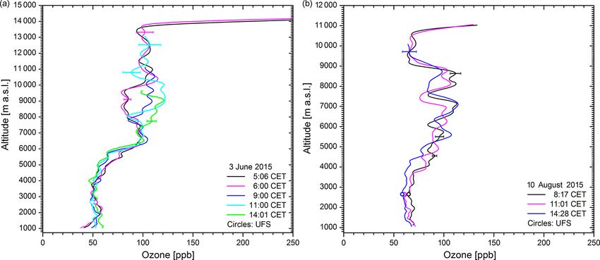
248                                                                          T. Trickl et al.: Very high stratospheric influence

to a longitude–latitude grid with 1◦ × 1◦ horizontal resolu-        case studies. HYSPLIT does not deliver potential vorticity.
tion. With respect to the vertical levels, ECMWF has used           Thus, a substantial air-mass descent was looked for in order
137 vertically hybrid levels since June 2013 (and 91 lev-           to identify a layer of stratospheric origin. If one or more tra-
els before), where 24 levels are between 250 and 600 mbar.          jectory bundles did not reach an altitude range typical of the
For each start time the 4 d forward trajectories are calculated     lower stratosphere in the outflow region of an intrusion (e.g.
starting in the entire region covering the Atlantic Ocean and       roughly 7.5 km or more in boreal regions) within 315 h, the
western Europe (20◦ east to 80◦ west and 40 to 80◦ north)           case was rejected. Just in a few cases extension trajectories
between 250 and 600 mbar. From this large set of trajectories       were calculated to verify the stratospheric source (Trickl et
those initially residing in the stratosphere (potential vorticity   al., 2015). For some case studies the FLEXPART model has
larger than 2.0 pvu) and descending during the following 4 d        also been used with a time span of 20 d (Trickl et al., 2014).
by more than 300 mbar into the troposphere were selected            FLEXPART produces a much more complex output beyond
as “stratospheric intrusion trajectories”. The same selection       the requirements of the current study, with thousands of mea-
criterion was used in a previous case study (Wernli, 1997)          surements.
to study an intrusion associated with a major North Atlantic           For many years we preferentially selected “reanaly-
cyclone.                                                            sis” meteorological data. Although the re-analysis data are
   Since June 2001 so-called “intrusion hit tables” have been       coarser than other meteorological data available, they have
additionally distributed that crudely estimate how strato-          led to a superior model performance in the free troposphere
spheric air develops over several days as a function of alti-       in many of our studies (Trickl et al., 2010, 2013, 2014;
tude above the four STACCATO (Stohl et al., 2003) partner           Fromm et al., 2010) and the analysis of our routine mea-
stations Jungfraujoch, Zugspitze, Monte Cimone and Thes-            surements. One additional example is discussed in Sect. 3.3.
saloniki. Both the STT trajectories and the hit tables are dis-     Despite the known limitations of backward trajectories (e.g.
tributed daily to all interested partners and institutions. In-     Stohl and Seibert, 1998), most specific free-tropospheric
trusion warnings based on these images have been issued by          ozone or aerosol layers in years of observations could be re-
IFU if several of the stations could be affected (Zanis et al.,     lated to reasonable sources, either in the boundary layer or in
2003b).                                                             the stratosphere. Since 2014 near-real-time data evaluation
   For special case studies LAGRANTO has been operated              and aerosol archiving in the EARLINET (European Aerosol
with re-analysis meteorological data, for periods up to 5 d         Research Lidar Network, https://www.earlinet.org, last ac-
(e.g. Trickl, 2014, 2016). The three-dimensional wind fields        cess: 2 January 2020) database have been achieved. Thus,
for the calculation of the trajectories were taken from the         GDAS-based trajectories (GDAS: Global Data Assimilation
ERA-Interim data set (Dee et al., 2011), which was inter-           System) have been taken since the re-analysis-based model
polated to a 1◦ × 1◦ horizontal grid and provides winds at 6 h      version are available only with considerable delay. The re-
intervals. The number of vertical levels in ERA-Interim is 60,      analysis mode was applied later on just if a GDAS run did
with 11 levels between 250 and 600 mbar.                            not verify STT.
                                                                       Slight vertical displacements of intrusion layers at the
2.2.2   HYSPLIT                                                     northern rim of the Alps exist in the model runs as re-
                                                                    ported previously (Trickl et al., 2010, 2015). These off-
For analysing intrusion events with travel times exceeding          sets, which vary from case to case, are explained by the in-
the 4 d set in the operational LAGRANTO forecast runs               sufficiently resolved orography that leads to an altitude of
or with source regions outside the domain of the forecasts,         IMK-IFU (730 m a.s.l.) roughly half-way between the val-
we use HYSPLIT (Hybrid Single-Particle Lagrangian Inte-             ley (Garmisch-Partenkirchen) and the Zugspitze summit. It
grated Trajectory, Draxler and Hess, 1998; Stein et al., 2015;      is important to activate the check box “terrain” on the HYS-
https://ready.arl.noaa.gov/HYSPLIT.php, last access: 2 Jan-         PLIT input page together with the “AMSL” (above mean sea
uary 2020) backward trajectories. HYSPLIT is easy to op-            level) altitude option. In this case, the absolute height is used
erate on the Internet and allows one to perform analyses of         on the vertical axis and the contours of mountains are dis-
the vertical profiles with an adequate expenditure of time in       played, and better agreement with the altitude of an arriv-
an intense programme of vertical sounding. We mostly used           ing atmospheric layer is achieved. The trajectories reproduce
the standard version with three trajectories initiated at dif-      air-mass lifting above mountain ranges, which is particularly
ferent altitudes within or close to a layer of interest, select-    spectacular above Greenland, with a surface altitude of about
ing the “model vertical velocity” option (three-dimensional).       3 km maintained over hundreds of kilometres.
These trajectories are extended over the maximum 315 h. If
necessary, several of these runs were started with slightly
varying initial conditions. Multi-trajectory ensembles have
also been used to create some “backward plume” (Trickl et
al., 2013). However, these ensembles did not cover a suffi-
cient number of days and have been applied in just a few

Atmos. Chem. Phys., 20, 243–266, 2020                                                  www.atmos-chem-phys.net/20/243/2020/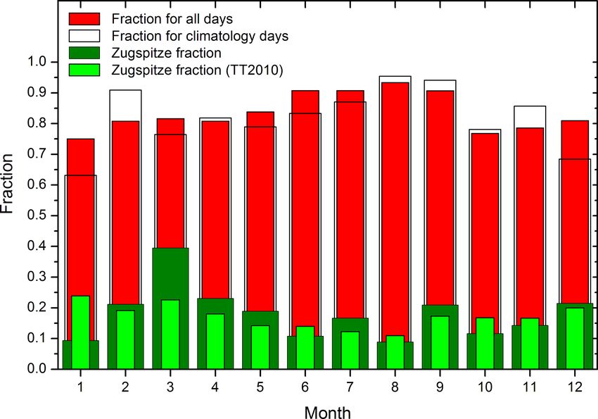
T. Trickl et al.: Very high stratospheric influence                                                                               249

Table 1. Measurement days with the ozone lidar between 2007 and 2016 (first line for a given year) and number of evaluated measurements
for a given month (second line); sumd: the number of measurement days; summ: the number of evaluated measurements.

                     Year      Jan   Feb    Mar    Apr    May      Jun    Jul   Aug    Sep    Oct    Nov     Dec
                     2007                             8      8       6                    2     8      7        7
                                                     21     50      15                    7    28     22       16
                     2008               4      3      7     11      5      1      7      2      9     12        5
                                       14     25     28     41      9      5     24     11     28     67       45
                     2009        8     10      1      9        1     4     9     11      3      7
                                45     63      1     46        2    12    49     56     19     51
                     2011                                                  4       1     5      6      6        1
                                                                          12       6    16     16     21        3
                     2012                                                                               1       2
                                                                                                        6       4
                     2013        2      6      2                     5    16       2    11     13      6       15
                                 3     21      8                    20    52       9    42     60     21       70
                     2014        9     16     20     10      8     18      9      8      9     14     13       12
                                37     59     64     39     22     43     27     24     28     34     40       36
                     2015       13     16     12     18      7      17     4     16     11     12     11
                                37     61     51     63     26      51    11     57     31     52     52
                     2016                                      2   10     11
                                                               4   54     45
                     Sumd       33     51     38     52     37     65     54     45     43     69     56       42
                     Summ      122   218     149    197    145     204   201    176    154    269    229     174
                     Total number of measurement days:                                                       585
                     Total number of evaluated measurements:                                                2238

3     Results                                                            There are several gaps in the data of the ozone DIAL.
                                                                      These gaps are explained by extended periods of laser or
3.1    Description of the data analysis and interpretation            computer damage, sometimes involving the search for new
                                                                      technical solutions for the system. The latest one occurred
In 2007, routine measurements have been started with both             between August 2016 and September 2017. These large gaps
DIAL systems. This has yielded vertical profiles of ozone,            do not exist for the water-vapour DIAL that was operated on
water vapour and aerosol backscatter coefficients, derived            298 d between 2007 and the end of 2014. Despite the subop-
from the 313 nm channel of the ozone DIAL. The number of              timal temporal overlap of both DIAL systems there are 120
measurements is particularly high in the case of the ozone            common measurement days during that period. On 108 of
lidar, resulting in a total of 2275 evaluated measurements            these days at least one intrusion was observed.
on a total of 585 d between 2007 and 2016 (Table 1). The                 Ozone is not always a good tracer of STT. Particularly
present study is, therefore, based on the ozone profiles dur-         in winter, small exceedances of the background ozone level
ing this period, and all other profile data are used for iden-        are frequently found in intrusion layers, related to a depar-
tifying the source for conspicuous ozone structures such as           ture from the lowermost layer of the stratosphere. These ex-
stratospheric air intrusions. Measurements have been made             ceedances can be resolved due to the high signal-to-noise ra-
on a large number of fair-weather days or during short pe-            tio during the cold part of the year with low ozone (40 ppb)
riods of clearing. However, really strong efforts to make at          and the resulting moderate absorption of the 277 nm radia-
least one measurement were limited to the EARLINET (Eu-               tion.
ropean Aerosol Research Lidar Network) “climatology days”                For identifying stratospheric intrusions, we primarily
Monday and Thursday (EARLINET, 2003). Ancillary infor-                looked for dry layers with RH ≤ 10 % (DIAL or sonde)
mation from sondes and trajectories has been gathered for             even if there was just as just a small indication of an ozone
each measurement day.                                                 rise. If ozone exceeded the neighbouring background by at

www.atmos-chem-phys.net/20/243/2020/                                                      Atmos. Chem. Phys., 20, 243–266, 2020
250                                                                                 T. Trickl et al.: Very high stratospheric influence

                                                                          the UFS data afterwards. As pointed out in Sect. 2.1.3, the
                                                                          Zugspitze RH rarely dropped clearly below 10 % due to an
                                                                          obvious bias.

                                                                          3.2   Typical findings

                                                                          As previously discussed (Trickl et al., 2010), stratospheric air
                                                                          intrusions passing over Garmisch-Partenkirchen arrive from
                                                                          almost all directions. Easterly directions mostly result from
                                                                          detours of the dry layers via eastern Europe or curl formation
                                                                          over central Europe potentially in cut-off lows.
                                                                             Intrusion layers can be observed under many different con-
                                                                          ditions. We routinely observe pre-fontal and post-frontal in-
                                                                          trusion layers, as well as intrusions slowly descending from
                                                                          the far west. The pre-frontal cases are frequently associated
                                                                          with stratospheric air masses descending from the Arctic to
                                                                          northern Africa or the Mediterranean basin followed by some
                                                                          return flow to central Europe. These layers normally rise
                                                                          as they are on a transition into a warm conveyor belt (e.g.
Figure 2. Vertical ozone profiles from the lidar measurements             Cooper et al., 2004). Post-frontal intrusions mostly reach low
on 1 October 2015; 235 ppb is the highest mixing ratio ever               altitudes above Garmisch-Partenkirchen and occur after vir-
measured with the IFU DIAL since the beginning of the mea-                tually all cold fronts, of course also in the “classical” case
surements in 1991. The distribution changes dramatically within           of beginning anti-cyclonic conditions (e.g. Stohl and Trickl,
about 10 h. The Munich thermal tropopause level was 10 454 m              1999; Trickl et al., 2003). They can, however, also occur be-
(00:00 UTC = 01:00 CET) and 11 903 m (12:00 UTC). The min-                tween two frontal passages that are sometimes separated by
imum sonde RH was 2 % (00:00 UTC) and 1 % (cut-off level,
                                                                          no more than 1 d. In these cases the inclined descending layer
12:00 UTC). The in situ data (1 h averages) of UFS (2670 m) are
                                                                          can be sandwiched between the low-lying clouds of the pre-
marked with circles coded in the same colours as the lidar measure-
ments next to the same time. A few error estimates representative of      ceding front and the high-lying clouds of the incoming new
the respective altitudes are given for a judgement of the data quality.   front.
                                                                             A few specific remarks:

                                                                           1. Very intense intrusions have been rare. Although intru-
least 10 % we analysed the respective layer with both LA-
                                                                              sions with 100–150 ppb of ozone in the middle and up-
GRANTO forward and HYSPLIT backward trajectories as
                                                                              per troposphere are not that rare, much higher values
described in Sect. 2.2. Such tiny ozone peaks were extremely
                                                                              are really exceptional. Just three cases with peak ozone
rare and, thus, almost did not affect the statistical results.
                                                                              mixing ratios reaching or exceeding 200 ppb have been
   The choice of RH = 10 % as the RH threshold is reason-
                                                                              found during the entire period described here (2007–
able since in most cases the minimum RH was clearly be-
                                                                              2016). The most intense intrusion, also covering a wide
low this value. In confirmation of our results from the water-
                                                                              vertical range, was observed on 1 October 2015 (Fig. 2).
vapour DIAL (Trickl et al., 2014, 2015, 2016), we found
                                                                              The peak ozone mixing ratio on that day was 235 ppb
typical minimum RH values of 1 %–3 % in the sonde data
                                                                              and rapidly dropped to less than 100 ppb. For compari-
for source regions over the North Atlantic or neighbour-
                                                                              son we give average values of the in situ GAW measure-
ing regions (intrusion Types 1–5 as defined by Trickl et al.,
                                                                              ments at UFS (2670 m). The ozone minimum at 12.2 km
2010, mostly by distinguishing source regions), 1 % being
                                                                              (07:52 CET) is close to the upper end of the operating
the lowest value found in the sonde listings (Sect. 2.1.4). For
                                                                              range of the lidar for these extreme concentrations, but
the most frequent long-range descent from a remote strato-
                                                                              is clearly visible and ascribed to the tropopause. This is
spheric source, e.g. central or western Canada, Alaska, or
                                                                              justified by the position of the Munich tropopause that
Siberia, Type 6 or slow descent from the North Atlantic min-
                                                                              descended from 13 341 to 11 903 m from midnight until
imum RH mostly ranged between 3 % and 6 %. Interestingly,
                                                                              noon.
the reverse also holds: finding sonde RH values in this range
very reliably points to very long transport times. Quite sur-                   The UFS ozone data exhibit a slight negative bias of 2 to
prisingly, the longest descent analysed (15–17 d) led to neg-                   4 ppb in the morning. This bias is outside typical differ-
ligibly low H2 O in the DIAL measurements at UFS (Trickl                        ences between the lidar and UFS or Zugspitze summit
et al., 2015, 16 July, 2013).                                                   and is ascribed to orographic lifting of the air masses
   Intrusions reaching altitudes around 3 km were verified by                   that arrived from the east (see below), along the former
looking at the Zugspitze ozone and RH data until 2010 and                       glacier basin.

Atmos. Chem. Phys., 20, 243–266, 2020                                                        www.atmos-chem-phys.net/20/243/2020/
T. Trickl et al.: Very high stratospheric influence 251
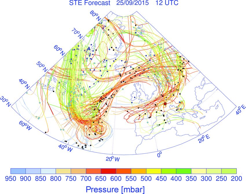
Figure 3. Recalculation of the LAGRANTO forward trajectories based on ERA-Interim wind data: the length of the trajectories is 5 d. Less
than 1 % of the trajectories are displayed for clearness. The pressure level is colour coded in mbar. The start time t0 is 25 September 2017,
12:00 UTC (13:00 CET), marked with dark blue dots. The times t0 + 2 d and t0 + 4 d are marked with bright blue and black dots, respectively.
The red dot north of the Italian peninsula marks the position of Garmisch-Partenkirchen.
Figure 4. DIAL ozone soundings on 30–31 December 2013 showing two narrow layers descending parallel to below 4 km a.s.l.
The presence of an intrusion on 1 October 2015 had time is slightly too early with respect to the lidar ob-
been predicted by the LAGRANTO operational fore- servations to avoid even higher complexity. However,
casts. For this paper the trajectory calculations were re- the principal advection path of the observed intrusion
peated with ERA Interim re-analysis data and extended remained for the later times and is explained in the fol-
from 4 to 5 d. In Fig. 3, we give one example for a lowing.
start time of 12:00 UTC (13:00 CET) on 25 September.
The trajectories clearly show a stratospheric intrusion Figure 3 and the trajectory plots for later times show
passing over Garmisch-Partenkirchen. The plot is rather high-lying and low-lying trajectories over southern
complex because several intrusions co-exist. This start Germany and qualitatively confirm the observations
in Fig. 2. The trajectories passing over Garmisch-
www.atmos-chem-phys.net/20/243/2020/ Atmos. Chem. Phys., 20, 243–266, 2020252 T. Trickl et al.: Very high stratospheric influence
Figure 5. Time series of ozone (a) and the 313 nm aerosol backscatter coefficient (b) on 31 January and 1 February 2014: Both a stratospheric
intrusion layer (6.5–9 km) and a weak to moderate Saharan dust event 2.5–6 km are seen. Due to a 3 h data gap between 19:00 and 22:00 CET
the colour coding during this period is highly uncertain. The intrusion could also have formed a full tropopause fold as indicated by the dashed
black lines.
Partenkirchen start over northern Greenland, pass over by Trickl et al. (2014) and verified by high-vertical-
(or near) Svalbard and then turn southward towards resolution FLEXPART transport modelling. Here, we
eastern Europe. This is exactly confirmed by the HYS- show as an example an even more exciting case from
PLIT backward trajectories that allow one to select start December 2013 of two parallel very thin high-ozone
times and altitudes above the lidar (not shown). The layers descending to Alpine summit levels (Fig. 4).
highest altitude (> 11 km) is reached above northern Again, the minimum RH was 1 %.
Greenland.
3. Slow long-distance descent (Type 6) dominates the ob-
Further exceptional mixing ratios were observed on servations above about 4.5 km. The slow descent of
26 February 2015 (235 ppb), and, in a particularly spec- stratospheric layers from remote source regions such as
tacular case (Trickl et al., 2014), on 6 March 2008 western Canada, Alaska or even Siberia down to Alpine
(200 ppb). summit levels was identified by Trickl et al. (2010).
These Type 6 intrusions were observed much more
2. Extremely thin layers can survive the long-range trans-
frequently above 4.5 km than at the Zugspitze sum-
port with almost negligible mixing. The width of in-
mit (see Sect. 3.4). A particularly spectacular case on
trusion layers can vary considerably from case to case.
16 July 2016 was analysed by Trickl et al. (2015): the
Layer widths clearly exceeding 2 km, in particular that
trajectories indicated a descent from the stratosphere
in Fig. 2, are not frequent, in agreement with the anal-
above Siberia over roughly 2 weeks without a resolvable
ysis of Colette and Ancellet (2005). Also very thin
rise in humidity. A source of STT can also be the sub-
layers with widths of down to 0.2 km have been ob-
tropical jet stream over Asia, reaching mid and high lat-
served. Both IFU DIAL systems are capable of resolv-
itudes over the Pacific Ocean (Trickl et al., 2011). This
ing these structures, and there is mostly very little mix-
kind of pathway was also found for some of our more
ing with tropospheric air (Trickl et al., 2014, 2015,
recent observations during the warm season.
2016). A particularly spectacular case (26–27 Decem-
ber 2008) of a thin, very dry (RH = 1 %, the obvious 4. Intrusion layers frequently arrive via northern Africa.
cut-off level of the sonde data) layer was discussed Long fronts reaching as far as the Sahara are typically
Atmos. Chem. Phys., 20, 243–266, 2020 www.atmos-chem-phys.net/20/243/2020/T. Trickl et al.: Very high stratospheric influence 253
Another dust case is shown in Figs. 7 and 8 for
18 June 2013, this time combined with long-range de-
scent from the northern United States (US) (and pre-
sumably beyond) and a single-loop curl at low latitudes,
with a corresponding trajectory analysis in Fig. 8. Here,
the intrusion air mass crossed the cold front over west-
ern Spain or Portugal. At 13:00 CET on 18 June this
front extended north–south from Bristol (UK) to north-
ern Africa. Obviously, the upper end of the clouds was
rather low in this area, similar to the May 1996 case
(Trickl et al., 2003). The RH determined from a compar-
ison of the results of the water-vapour DIAL (Fig. 7b)
and the Munich radiosonde was 8 % to 12 %. These
rather high values are ascribed to the very long descent
during at least 13 d.
Intrusions co-existing with Saharan dust were observed
on a total of 67 d. The number of dust days in our record
is limited because frequently dust arrives below clouds,
which impedes lidar measurements.
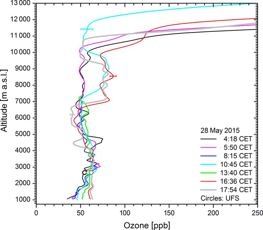
5. Summer-time ozone in the middle and upper tropo-
sphere has been frequently high. Elevated ozone was a
feature observed many times above about 4.5 km dur-
ing the warm season. Two examples from May and Au-
gust 2015 are shown in Fig. 9. In both cases (and most
others) dry layers exist within the high-ozone range and
Figure 6. Selected HYSPLIT 315 h backward trajectories starting the corresponding HYSPLIT trajectories stay at high
above Garmisch-Partenkirchen on 1 February 2014 at 00:00 CET altitudes. For the altitudes in these examples analysed
within the two aerosol layers in Fig. 5 (lower panel) between 3 and
with trajectories we did not find any contact with poten-
4.5 km as well as in the stratospheric intrusion between 6 and 9 km
tially polluted planetary boundary layer (PBL) within
(upper panel in Fig. 5); the black curves at the bottom of the vertical
cross section mark the ground levels for each trajectory. the maximum of 315 h provided by the model. How-
ever, the calculation for a cirrus layer around 7.5 km on
10 August ended around 5 km over the Pacific, giving
associated with the advection of dust (Papayannis et al., some hint on the origin of the moisture required for the
2008). Pre-frontal intrusion layers have been mostly lo- cloud formation.
cated above the dust layer (exceptions exist). In Fig. 5
we show time series of the ozone aerosol profiles on 6. Volcanic and fire aerosol are transported downward
31 January and 1 February 2014, and Fig. 6 displays from the lowermost stratosphere. During the periods
three HYSPLIT trajectories selected for the three rele- of major volcanic activity impacting the lower strato-
vant ozone and aerosol layers at midnight between the sphere, aerosol was frequently detected in intrusion
two days. The dust was lifted to roughly 5 km, which layers (see also Browell et al., 1987). More specifi-
is typical of these Föhn events at the northern rim of cally, particles in intrusion layers were registered after
the Alps (e.g. Jäger et al., 1988). Above the dust lay- the eruptions of Okmok and Kasatochi (July and Au-
ers a layer with elevated ozone passed over Garmisch- gust 2008, respectively; see Trickl et al., 2016), Re-
Partenkirchen. The minimum Munich RH on 1 Febru- doubt (March 2009), Sarychev (June 2009) and Nabro
ary at 01:00 CET was 2 %, indicating a moderate travel (June 2011) (more details: Trickl et al., 2013). Typ-
time (the UFS DIAL was not operated). The intrusion ical 313 nm aerosol backscatter coefficients were 5 ×
trajectory in Fig. 6 shows rather rapid transport from 10−7 m−1 sr−1 and less. The highest value was 2.35 ×
about 10 km above Cape Farvel (Greenland) to north- 10−6 m−1 sr−1 , observed on 7 September 2009 after
ern Africa. Obviously, this high speed makes it possi- the violent eruption of Sarychev. Stratospheric intru-
ble to pass eastward over the southern part of the front sions have been identified as a highly important mech-
and enter the air stream rising to the Alps. The LA- anism for the rapid depletion of stratospheric aerosol in
GRANTO STT forecast confirms at least subsidence the mid-latitudes within 1 year or less (Deshler, 2008;
from Labrador to northern Africa. Trickl et al., 2013). This includes strong fires (pyro-Cbs)
that normally just reach the lowermost stratosphere (e.g.
www.atmos-chem-phys.net/20/243/2020/ Atmos. Chem. Phys., 20, 243–266, 2020254 T. Trickl et al.: Very high stratospheric influence
Fromm et al., 2008, 2010), the latest presumable smoke that the air quality in the United States (US) has improved.
case being 2 October 2017 for the strong fires in British Nevertheless, we did identify several cases of intercontinen-
Columbia that were observed up above our site to an ex- tal transport of pronounced amounts of ozone. One of these
ceptional 20 km (not shown). Tropospheric smoke has cases is described below. In general, a clear distinction of
also been found in intrusions (Trickl et al., 2015). long-range advection from the stratosphere or a polluted PBL
is a complex task beyond the scope of this paper. It requires
7. Dry air layers can also arrive from the lower-latitude more suitable analysis tools such as the FLEXPART model as
Atlantic. Quite a few of the dry layers with elevated applied by us in detail in previous studies (e.g. Trickl et al.,
ozone have been traced back to the south-west of the 2003, 2010, 2011). There, we extended FLEXPART-based
Azores. Here, the trajectories frequently form curls or analyses to up to 20 days and found merging air streams from
spirals exiting backward towards the north-west (e.g. the stratosphere and remote boundary layers (Trickl et al.,
Fig. 8). In several cases extension trajectories were cal- 2011).
culated and confirm descent from high altitude at high It is very difficult to estimate the stratospheric contribution
latitudes. Only these verified cases were accepted as in the summertime middle and upper troposphere. The sonde
“stratospheric”, given the low humidity. data show very low humidity mostly in rather confined lay-
8. Intrusions rarely penetrate into the PBL. During the ers and rarely in the entire range with elevated ozone. This
past decade there has been enhanced interest in the role can indicate mixing in merging air streams, but could also
of STT in air quality (e.g. Lefohn et al., 2011; Lang- be attributed to differences in vertical distribution with re-
ford et al., 2012; Lin et al., 2012, 2015). We have rou- spect to the rather remote radiosonde stations. In the case of
tinely observed ozone peaks below 2000 m, but have not mixing, an assessment of the stratospheric component would
analysed penetration of intrusions into the PBL in detail have to rely on model-based estimates, which can be rather
because of the absence of water-vapour measurements crude (e.g. Trickl et al., 2014).
below 3000 m that could identify intrusions even with- As one example of a significant North American ozone
out pronounced ozone structure. However, we have ob- plume we describe here the case of 28 May 2015. On that day
served intrusions sliding along the top of the PBL over a major part of the summertime ozone step could be related
several days without a clear indication of penetration to a high-ozone episode in the eastern US. Again, a part of
into it. This suggests that descent towards the ground is the step (the lowest section) is related to STT. The ozone pro-
likely to occur mostly during night-time at the end of files from that day are displayed in Fig. 10. At almost all tro-
the primary subsidence. This could explain why Reiter pospheric altitudes there were (in part remarkable) changes
et al. (1990), based on years of ozone soundings with the in ozone that could be explained by the RH and trajectory
Eibsee-Zugspitze cable car (1.0 km to 2.95 km a.s.l.), analyses. In the morning two intrusion layers from source re-
did not observe any case of subsidence to below 1.4– gions around Alaska are discernible at about 4.7 and 3.1 km
1.6 km a.s.l.: the cable car runs only during day-time. In (RH = 6 % and 4 %, respectively). The trajectories seem to
fact, Eisele et al. (1999) reported a case of sufficiently continue rising for backward times beyond −315 h to alti-
deep early-morning descent of a STT layer that it could tudes higher than 7 km. These intrusions diminish later on.
be caught by the forming PBL. Similar conclusions are In the afternoon an ozone step to roughly 80 ppb formed
reported by Ott et al. (2016). above 6.7 km (light blue, red and grey curves in Fig. 10).
The air mass was rather humid (Munich sonde RH 50 %–
3.3 STT and long-range transport of boundary-layer 76 % at 13:00 CET; some backscatter profiles showed signal
ozone from cirrus clouds), with the exception of the lowest peak
for which the Munich radiosonde yielded RH = 4 % (there
The typical ozone rise to sometimes even more than 100 ppb at 7.6 km). Figure 11 shows three 315 h HYSPLIT back-
in the middle and upper troposphere during the warm sea- ward trajectories selected for relevant altitudes above our site
son mentioned in Item 5 of Sect. 3.2 is remarkable. Since (7400, 8200, 8500 m) from a larger number of trajectories
such behaviour is mostly absent during the darker period of calculated. The ozone rise near 7 km corresponds to long-
the year, this could suggest that a higher ozone background range descent from northern Alaska, in agreement with the
due to strong photochemical activity is imported from remote low RH.
regions such as North America or East Asia. An analysis The higher trajectories bend southward over the Great
carried out in 2005 based on FLEXTRA (e.g. Stohl et al., Lakes and follow the Mississippi back to the Caribbean
1998) trajectories limited to just 8 d backward in time yielded Sea. On 24 May an altitude of 1.5 km is reached, i.e. above
North American influence over Garmisch-Partenkirchen dur- Louisiana. The strong air-mass rise from the Gulf of Mexico
ing already 28 % of the time for the period April 2003– to Canada suggests the presence of a warm conveyor belt.
September 2004 (ATMOFAST, 2005). Indeed, we verified the presence of a rather wide warm con-
Since we did not analyse vertical ranges with constant veyor belt with tools described by Madonna et al. (2014)
moderate ozone for the period since 2007, this could suggest and Sprenger et al. (2017). To the east a wide zone with
Atmos. Chem. Phys., 20, 243–266, 2020 www.atmos-chem-phys.net/20/243/2020/T. Trickl et al.: Very high stratospheric influence 255
Figure 7. Profiles of ozone, the aerosol backscatter coefficient (a) and the water-vapour number density n (b) from DIAL measurements
at IFU and UFS on 18 June 2013 during a Saharan dust event; the 250 m upward displacement of the humidity minimum with respect to
the ozone maximum is ascribed to orographic effects. For comparison, the densities for RH = 30 % and the measured RH by the Munich
radiosonde are shown. The stratospheric intrusion peak at around 5.7 km corresponds to 8 %–12 % RH because of long-range descent (Fig. 8).
The times specified for the UFS DIAL are the end times of the respective measurement (lasting about 16 min). The in situ data of UFS
(2670 m) are marked with circles coded in the same colours as the lidar measurements next to the same time and confirm the values from the
lidar measurements within 1–2 ppb.
peak ozone exceeding 80 ppb is revealed in Fig. 12, in- with the nearby H2 O DIAL are adequate. However, they were
dicating long-lasting high pressure. Ozone maps from the not always made on the same day and sometimes not even
US Environmental Protection Agency (https://www.epa.gov/ within the same range of hours, which reduced the number
outdoor-air-quality-data/, last access: 2 January 2020) con- of intrusion cases on which the stratospheric ozone content
firm a moderate ozone rise, particularly over Illinois and could be determined. Radiosonde data can only be used as a
Kentucky exactly on 23 May. The trajectories propagate qualitative tool to verify the presence of an intrusion layer in
along the western side of the high-ozone zone in Fig. 12 and the region due to the long distance to the stations.
indicate some overlap with this region. This result is rather As a consequence, we decided for the current study to
satisfactory and confirms our excellent experience with the perform a statistical analysis of the fraction of the measure-
HYSPLIT run with the re-analysis option. In fact, we also ment days per month with one more identified intrusion layer
tested the GDAS option that offers better spatial resolution. (Sect. 3.1), similar to the approach by Beekmann et al. (1997;
As in earlier comparisons (e.g. Trickl et al., 2016), we found see Sect. 4). The seasonal cycle from our analysis is shown
strong deviations from Fig. 11, with almost all trajectories in Fig. 13, based on all (585) measurement days for each
leading backward to Alaska at high altitudes, approximately month between 2007 and 2016. The month-to-month varia-
parallel to the red 7400 m trajectory in Fig. 11. This result tion of the fractions is rather low. We derived a standard de-
is in considerable disagreement with the RH data that show viation of the fraction from months with at least 8 measure-
a narrow dry layer just above 7 km and elevated humidity at ment days. The resulting overall standard deviation was 0.12,
higher altitudes that is in excellent agreement with the import which looks unrealistically high considering the smoothness
from the Caribbean Sea suggested in Fig. 11 and the cirrus of the data in Fig. 13 and is ascribed to the reduction of the
signal in the lidar backscatter data. data set in this procedure.
In order to demonstrate that there is no bias due to the
3.4 Statistical analysis of STT choice of the measurement days, we also show the results
for Monday and Thursday, i.e. the EARLINET “climatology
The ozone profiles alone do not allow us to quantify free- days” (a total of 286). Due to the reduction in days, the vari-
tropospheric ozone budget due to STT. The boundaries of ability is higher. Nevertheless, the principal course of the sea-
the intrusion layers cannot always be clearly distinguished. sonal cycle is retained and no significant bias is seen. Just for
Water-vapour profiles show a clearer contrast and can be used the period December to February the deviations are larger
for identifying the range of the STT layers. The soundings due to a smaller number of climatology days covered.
www.atmos-chem-phys.net/20/243/2020/ Atmos. Chem. Phys., 20, 243–266, 2020You can also read