MARINE CLOUD BRIGHTENING - UW Atmospheric Sciences

MARINE CLOUD BRIGHTENING

Authors:- John Latham1,4 , Keith Bower4 , Tom Choularton4 , Hugh Coe4, Paul Connelly4 , Gary
Cooper7 ,Tim Craft4, Jack Foster7, Alan Gadian5, Lee Galbraith7 Hector Iacovides4 , David
Johnston7 , Brian Launder4, Brian Leslie7 , John Meyer7, Armand Neukermans7, Bob Ormond7,
Ben Parkes5 , Phillip Rasch3, John Rush7, Stephen Salter6, Tom Stevenson6, Hailong Wang3, Qin
Wang7 & Rob Wood2 .

Affiliations:- 1 National Centre for Atmospheric Research, Boulder, CO. 2 U Washington, Seattle,       3

PNNL, Richland, WA., 4 U Manchester, 5 U of Leeds, 6 U of Edinburgh, 7 Silver Lining, CA.

Abstract

The idea behind the marine cloud brightening (MCB) geoengineering technique is that seeding
marine stratocumulus clouds with copious quantities of roughly monodisperse sub-micrometre
seawater particles could significantly enhance the cloud droplet number concentration thus
increasing the cloud albedo and longevity – thereby producing a cooling, which computations
suggest could be adequate to balance the warming associated with a doubling of atmospheric
carbon dioxide.

We review herein recent research on a number of critical issues associated with MCB: (1) general
circulation model (GCM) studies, which are our primary tools to evaluate globally the effectiveness
of marine cloud brightening and to assess its climate impacts on rainfall amounts and distribution,
as well as on polar sea-ice cover and thickness: (2) high resolution modeling of the effects of
seeding on marine stratocumulus, which are required to understand the complex array of
interacting cloud processes involved in brightening: (3) microphysical modelling sensitivity studies
examining the influence of seeding amount, seed-particle salt-mass, air-mass characteristics,
updraught speed and other parameters on cloud-albedo change: (4) sea-water spray production by
controlled electrohydrodynamic instability, and by microfabrication lithography: (5) computational
fluid dynamics studies of possible large-scale periodicities in Flettner rotors: and (6) the planning
of a three-stage limited-area field research experiment, which has the objective of developing our
fundamental knowledge of marine stratocumulus clouds, testing the technology developed for the
MCB geoengineering application, and ultimately, if deemed justifiable, field-testing the idea
quantitatively, on a limited (perhaps 100km) spatial scale.

KEYWORDS: cloud brightening: albedo: GCM and high resolution modeling: cloud seeding:
spray technology: field experiment

1.. Introduction

Cloud-brightening, one of several Solar Radiation Management (SRM) geoengineering ideas
involving the production of a global cooling to compensate for the warming associated with
continuing fossil fuel burning, was first postulated by Latham (1990, 2002). The ideas, engineering
requirements, and climate impacts associated with cloud brightening have been significantly
explored by Bower et al. (2006), Salter et al. (2008), Latham et al. (2008) and Rasch et al. (2009),
Jones et al. (2009, 2010), Korhonen et al. (2010) , Bala et al. (2010) and Wang et al (2010).
.

                                                                                                    1

The basic principle behind the idea is to seed marine stratocumulus clouds with seawater aerosol
generated at or near the ocean surface. These particles would have sufficiently large salt-mass to
ensure their subsequent growth within the clouds without being so large as to encourage
precipitation formation, and would be sufficiently numerous to enhance the cloud droplet number
concentration to values substantially higher than the natural ones, thereby enhancing the cloud
albedo (Twomey, 1977). Enhancing the droplet concentration is likely also to affect the cloud
macrophysical properties such as cloud cover, longevity, liquid water content and thickness, as a
consequence of inhibiting precipitation formation (e.g. Albrecht 1989) and the timescale for the
evaporation and sedimentation of cloud droplets.These feedbacks on the cloud properties can
result in secondary aerosol indirect effects that are poorly understood and represent a major
challenge in the general problem of understanding and quantifying how aerosols impact the
climate system (Lohmann and Feichter 2005, Stevens and Feingold 2009, IPCC 2000).

Climate model simulations suggest that if the droplet concentration in marine stratocumulus can be
increased to several hundred droplets per cm3 in a significant fraction of the stratocumulus sheets,
then, in principle, a negative forcing can be produced, sufficient to offset doubled CO2 and
maintain the polar sea-ice coverage at roughly current values. If this was achieved, the global
distributions of surface temperature and sea-ice cover would inevitably be different from the
present situation. Also, as demonstrated by the computations of Rasch et al (2009), the negative
forcing required to hold the Earth’s average surface temperature at the current value (in the face of
CO2-doubling) would be different from that required for average sea-ice coverage maintenance
(which would in fact be different at the two poles).

The principal objectives of this paper are to assess the current state of all significant aspects of
recent work that we and others have conducted on MCB, to identify the major unresolved
problems, and to outline our plans for further development of our work in these most important
areas. We also hope to make it clear that the effective further development of our geoengineering
study requires a comprehensive programme of fundamental research in several arenas, especially
cloud physics.

The change in cloud albedo resulting from seeding the clouds with seawater particles large enough
to be activated is roughly proportional to ln(N/No) (Twomey, 1977), where No and N are
respectively the background droplet number concentration (prior to seeding) and the post-seeding
value. No is therefore a critical parameter in determining the albedo enhancement resulting from
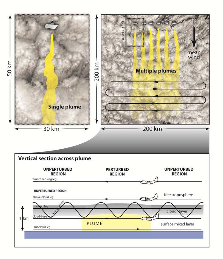
seeding, so it is crucial to obtain accurate values of it, over the oceans. Recent observational work
by Bennartz (2007), and Wood et al (2010), based on data from the NASA MODIS satellite
instrument and airborne measurements in the VOCALS field experiment, are beginning to provide
a reliable global assessment of No that has not been evaluated hitherto. These findings are
illustrated in Figure 1.

                                                                                                     2

Figure 1. Panel (a): Map of MODIS-derived annual mean cloud droplet concentration N0 for
stratiform marine warm clouds. To be included in the annual mean, the daily warm cloud fraction in
1x1 degree boxes must exceed 50% to capture primarily marine stratocumulus clouds. Panel (b):
Cumulative distribution of daily 1x1 degree droplet number, N0 from MODIS for all ocean points.
Panel (c): Comparison of MODIS and C-130 aircraft measured cloud droplet concentration
estimates from the VOCALS Regional Experiment during October/November 2008 off the Chilean
coast (Wood et al. 2010), for longitudes 70-77.5W (more polluted) and 77.5-85W (more pristine).
There is good agreement between in-situ and satellite-derived values which lends weight to the
use of these data over the global oceans.

The sections into which the paper is divided are: (a) GCM modeling of the cloud brightening
scheme, and its influence on rainfall amounts and distributions, as well as sea-ice cover and
thickness: (b) parcel modelling and its technological applications, (c) high-resolution cloud
modelling: (d), spray production technologies under current investigation and Flettner rotor CFD
modelling: (e), planning of a limited-area field research experiment, which has the objectives of
developing our fundamental knowledge of marine stratocumulus clouds, and testing both MCB and
the technology developed for this geoengineering application: (f) discussion.

2.   Global Climate Modelling: Precipitation and Ice cover.

The objective of this section is to use the UK Met Office climate model, HadGEM1, (Hadley Centre
Global Environmental Model) to study some climatological impacts of changing the cloud
condensation nucleus (CCN) concentration in defined maritime oceanic regions which have

                                                                                                 3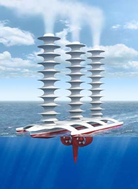

significant stratocumulus sheets. We present studies of the influence of this seeding on global
precipitation and polar sea ice extent and thickness. There have been several GCM studies of
MCB since the first atmosphere-only simulations, Latham et al., 2008). HadGAM, an
atmosphere only climate model, has the advantage of an immediate response to greenhouse gas
forcing, and can provide an immediate change in the Top of Atmosphere (TOA) radiative forcing. It
is limited by having no component of ocean meridional heat transport flux and circulation. Slab
GCM's have the advantage that short time scale thermocline changes are simulated. This can be
suitable for NWP purposes, but is of limited representativity in climate studies. Fully coupled
ocean-atmosphere GCM's include the large scale oceanic meridional heat transport, but the long
time-constant ocean circulations provide the challenge of large scale hysteresis for the climate
system. Jones et al (2009, 2010) used the UK Met Office HadGAM and HadGEM1 models. Bala
et al (2010) and Rasch et al (2009) used the NCAR Community Climate System Model. In section
2.1, changes in precipitation resulting from seeding are discussed. In section 2.2, new results are
presented on its impacts on ice thickness and ice extent.

The HadGEM1 model employed in our current studies is based on version 6.1 UK Met Office
Unified Model (UM), with an atmospheric resolution of 1.25 by 1.875 degrees with 38 vertical
levels, an upper lid at 39 km, and a coupled ocean model of variable grid size from 1 degree
squares at the poles to 1/3rd of a degree at the Equator and to a depth of 5.3km using 40 levels. An
emphasis in these models is on the improvement in the cloud and stratocumulus mixing
parameterisations and this has been particularly useful in MCB studies, enabling improved
calculations to be made of cloud droplet effective radius, radiative forcing and liquid water path
(Martin et al. 2006). They have also provided the ability to focus on precipitation, surface
temperature, cloud and sea surface temperatures, ice fraction and depth. HadGEM1 was used in
the IPCC 2007 report (IPCC Working Group 1, 2007). The A1B case, is a standard scenario where
technological developments are “balanced” and defined as not relying too heavily on fossil or non-
fossil energy sources and also based on the assumption that similar improvement rates apply to
both energy supply and end-use technologies.

With one exception, the results from previous simulations, and our own, show a significant
increase in albedo in a seeded climate environment equivalent to compensating for an
approximate doubling of planetary atmospheric CO2. For the atmosphere only HadGAM
computations, the equivalent TOA negative forcing is about -3.7 W/m2 . The computations of
Korhonen et al. (2010) predict smaller values of albedo-change and associated negative forcing
but this is probably due to the fact that they used values of No which were between 2 and 3 times
higher than the experimentally determined values for unpolluted regions presented in Figure 1.
Simple calculations using the Twomey equations confirm that if their values of No are reduced by a
factor of 2 or 3, the resulting values of negative forcing are roughly consistent with those of other
workers.

In our study, three simulations were completed, each for 70 years from 2020 to 2090, with the last
20 years analysed; a control run with static carbon dioxide at 2020 levels (435ppm), a run with
increasing carbon dioxide by 1%/year up to double pre-industrial carbon dioxide levels (560ppm at
2045).Case A was the control based on current (2020) carbon dioxide levels (435ppm).Case B
was the control run plus 1% CO2 increase p.a., until double pre-industrial levels (560 ppm) were
reached, at which point the CO2 levels were held static. Case C was as B, but with seeding of
N=375cm-3 in three limited regions, off the Western coasts of California, Peru and Namibia, which
Jones et al. (2009) highlighted as being particularly effective, due to their propensity for
stratocumulus cloud fields in our current climatology.

2.1. Precipitation

The recent results from climate simulations cited above have shown variations in modelled
precipitation when cloud seeding schemes have been introduced. The discussion here will focus
on why this occurs, how these model results differ, and their significance.

                                                                                                    4

Precipitation is not well described in climate models. The CPC Merged Analysis of Precipitation
   (CMAP) dataset provided by NOAA (Xie & Arkin, 1997) for 1979-2000 was compared with a ten
   year simulation using current static carbon dioxide levels. Figure 2a shows the difference between
   precipitation rate in HadGEM1 and the CMAP data set. The globally averaged difference in
   precipitation rates over land is 0.17 mm/day. Across most of the Northern land masses the
   precipitation difference is less than 1 mm/day. In the tropical regions the model does not well
   reproduce measured values downwind of particularly the South East Asian and South American
   mountain ranges. Across the globe the model is weakest in the presence of steep mountain
   ranges, on the West of a continental region. The increased precipitation on the upwind steep
   slopes produces an impact on the availability of water vapour in the lee of the mountains. It is
   within these limitations that results regarding precipitation patterns in a future seeded or non-
   seeded climate should be considered.

Figure 2a. Difference in precipitation between          Figure 2(b). Difference in precipitation
CMAP and HadGEM1 simulations for current                resulting from simulations C – A (seeding of
climate conditions. The units are mm/day. The           the three regions of stratocumulus - with
global difference over land is 0.17mm/day. There        current conditions). Units are mm/day. This
are discrepancies in modelled precipitation in some     plot shows the precipitation differences that
tropical regions and near steep orography.              could occur in a geoengineered scenario

   The difference in precipitation between simulations for seeded and control state A1B, CO2
   simulations (C and A), Figure 2(b), is similar to Figure 4(b) in Jones et al (2009), Figure 3(b) in
   Rasch et al (2009) and Figure 7 in Bala et al (2010). Although each model has used a different
   seeding strategy, there is some degree of overlap. In cases where the whole maritime cloud has
   been seeded, the results do not on average differ significantly. Of course, this may be a function
   of the fact that climate models can have similar rainfall parameterisation schemes, but
   alternatively it may represent a realistic feature. The reduction of precipitation in Figure 2(b) for
   the whole averaged Amazon basin is consistent with that of Jones et al. (2009, 2010), but the
   decrease is much smaller in magnitude. However, for the whole of this region, the rainfall
   reduction is about the same as the errors in current model simulations compared with CMAP data,
   Figure 2(a), and is a result of the unrealistically large precipitation values in the desert area West
   of the Andes. Thus, the Jones et al (2010) results should be treated with caution in this region.
   Excess precipitation on upwind steep slopes removes downwind available atmospheric water
   vapour. This reduction is not present in Rasch et al (2009), but they seed a much larger portion of
   the ocean. The results of Bala et al. (2010), who seeded all suitable clouds, exhibit no significant
   Amazonian rainfall reduction, and globally indicate a small increase in precipitation over land. We
   note that our Case C simulation shows a relative increase in precipitation across sub-Saharan
   Africa and India. African and Indonesian precipitation increases are present in Rasch et al (2009).
   Bala et al (2010) find no significant reduction in precipitation in any land region. Recent results of
   Jones et al (personal communication), have indicated that their reduction in rainfall in the Amazon

                                                                                                        5

region is a consequence of their seeding of the Southern Hemisphere stratocumulus cloud
region, but the reason for this is not clear.

To summarise, one of the most difficult challenges in climate modelling is to predict more
accurately global precipitation patterns. Our results show a small increase in precipitation in the
dryer regions of Africa as indicated in Figure 2(b), with a small average decrease in the Amazon
region. These results from our model indicate that there are changes in precipitation produced in
the seeding cases, but that the variations are within the bounds of current model precision and
uncertainties. Higher resolution and more accurate simulations are clearly required for future work.

2.2.. Sea Ice Extent and Thickness

The three maritime regions were seeded in a similar pattern to Jones et al. (2009, 2010). Figures 3
and 4 show the change in the summer minimum sea ice fraction and sea ice thickness
respectively. The Arctic ice minimum has been taken to occur in September and the Antarctic
minimum in March. All data has been taken from the final 20 years of the 70 years simulations.

Figures 3(a) and 3(b) show the significant reduction in sea ice fraction under a doubling of pre-
industrial carbon dioxide atmosphere, Case B. There is a general and significant loss of sea ice in
Polar regions. In the Southern Hemisphere, Figures 3(b) and 3(d) the reduction in sea ice is non-
uniform, with the most significant reduction to be found East of the Antarctic Peninsula. The Arctic
ice minimum in the double CO2 scenario, Figure 3(a), Case B – Case A, is a 76% reduction from
the 2020 ice extent, but with seeding switched on, Figure 3(c), Case C – Case A, the reduction is
only 3%. In the Southern Hemisphere, Figures 3(b) and 3(d), the equivalent reductions are 30%
and 17%.

In contrast, with the above, the sea ice depth increases close to the North Pole, Figures 4(a) and
4(c) creating a small central region of thicker ice in the double CO2 scenario, and to a much lesser
extent in the seeded scenario. This corresponds to a model increase in precipitation in this polar
region. In the Southern ocean the changes are non-uniform and - in some existing ice regions -
there is an increase in the South Polar minima sea ice thickness.

There are several major regions where the sea ice thickness is reduced by more than 2m, Figure
4(b), and again a lesser extent in the geoengineered case Figure 4(d). This is consistent with a
southward movement of mid latitude weather patterns. The representation of the melt rate of
glaciers is of concern since the current climate models seem unable to represent the observed
more rapid change. It is therefore likely that the loss of ice may occur at a greater rate than current
model predictions, 30% as cited above, for the double CO2 scenario. With seeding on, at the North
Pole, there remains an increase in sea ice thickness at the North Pole, but a marginal change at
the South Pole.

In summary, taking both the ice fraction and depth characteristics together, seeding significantly
reduces the sea ice fraction loss during the summer months. The Southern minima reduction in
sea ice fraction is smaller than in the Northern Hemisphere. The increase in sea ice thickness
near the pole in the geoengineered scenario does not alter the albedo of that region. Further, not
shown here, there is a possible feedback effect which has not been included in the modelling. In
the Northern Hemisphere Case C, there is an increase in sea ice fraction to the North of Siberia
which increases the albedo relative to the control. The changes in ice cover fraction are
consistent with those of Rasch et al (2009), but the reduction of the Southern Hemisphere ice
fraction is smaller in our calculations. The simulations indicate that our seeding with N=375cm-3 ,
increases ice extent in the double CO2 scenario. Results from seeding all the oceans, not
presented here, produces a further enhancement of planetary albedo and growth of polar ice cover
compared with the control scenario.

                                                                                                      6

(a)              (c)

       (b )
      (d)

      Figure 3. Comparison of the North and South
      polar sea ice fraction averaged over the summer
      minimum for the final 20 years of the 70 year
      simulations. Northern minimum is taken as
      September, and the Southern minimum is taken
      as March. Panels (a) & (b) show the difference
      in North and South polar sea ice fraction
      between Case B and Case A. Panels (c) & (d)
      show the difference in North and South polar sea
      ice fraction between Case C and Case A

                                                     7

(a)                                                     (c)

  (b )                                                  (d)

Figure 4. Comparison of the North and South polar sea ice thickness averaged over the summer
minimum for the final 20 years of 70 year simulations. Northern minimum is taken as September,
and the Southern minimum is taken as March. Panels (a) & (b) show the difference in the North
and South polar sea ice thickness between Case B and Case A. Panels (c) & (d) show the
difference in the North and South polar sea ice thickness between Case C and Case A

3. Cloud Modelling Relevant to Spray Characteristics and Albedo-Change Values

The purpose of this section is to explore the range of dry salt masses and concentrations that are
most effective for altering the albedo of marine boundary layer clouds.

3.1 Explanation of model and set up of runs

We have used a new cloud parcel model with size resolved or bin microphysics that has been
developed at Manchester and is called ACPIM (Aerosol-Cloud and Precipitation Interactions
Model) (see e.g. Connolly et al, 2009). The work we have carried out here builds on that previously
reported in Bower et al., (2006). In their work, the composition of the background aerosol size
distributions and that of the added aerosol particles was prescribed to be sodium chloride. The
added particles also had a single monomodal size. In this work, the size distributions of the
background aerosol distributions are the same as in Bower et al., (2006) but are comprised of
ammonium sulphate to which sodium chloride particles are added in a mode of finite width to
replicate more realistically the size distributions of particles that can be generated by the spray
production techniques described in sections 5.2 and 5.3. The lower limit of added salt particle
mass in Bower et al., (2006) was 10**-18 kg, sufficient to cover the range of dry particle sizes
under consideration at the time (Salter et al., 2008). However, the range of the mass of added salt
particles has now been extended to smaller sizes, to encompass the size-range that can be
produced using the Taylor-cone technique (described later), which produces dry salt particles in
the mass range ~3.10**20 to 5 x 10**19kg.

The parcel model version of ACPIM used here activates aerosols in a sectional way. ACPIM also
uses a more thorough description of the thermodynamics of the aerosol (Topping et al 2005) than
                                                                                                     8

was present in the NEATCHEM model used in the Bower et al., study. Three sets of model runs
were performed with ACPIM; in each set of runs the control corresponded to running the model
with a `background’ aerosol size distribution measured in three different air masses (the clean,
medium and dirty distributions used in Bower et al., 2006). Clean corresponds to a total number
concentration of ~10 cm-3; medium ~260 cm-3 and dirty ~1000 cm-3.

Koehler theory was used to determine the equilibrium vapour pressure of the aerosols (see
Topping et al., 2005) in the background size distribution of particles (composed of (NH4)2SO4). The
initial relative humidity, pressure and temperature in the model were set to 95%, 950 hPa and
283.15 K respectively and the model was run until the parcel was lifted a total of 250m. Typically
this generated a cloud base (ie saturation level) ~75m above the starting level and hence a cloud
~175m deep, allowing comparison with the results of Bower et al.(2006) Future work will look at
the sensitivity of the addition of aerosols to deeper (ie more optically thick) clouds, although (as in
the Bower et al. studies) the trends in albedo changes produced are expected to be similar. These
simulations were repeated for different prescribed vertical wind-speeds of 0.2ms-1, 0.5ms-1 and
1.0ms-1 to represent the typical range of updraft speeds found in marine stratocumulus. Sensitivity
tests were then performed investigating the effect of adding a log-normal mode of aerosol to the
background ammonium sulphate aerosol distributions to simulate the spread in sizes expected
from the droplet spray technique. The composition of the particles in the added aerosol mode was
NaCl, and their equilibrium vapour pressures were obtained from Koehler theory.

The parameters varied in these tests were the total number of added aerosol particles, nadd, and
their dry salt mass ms. The parameter values used were nadd=0, 30, 300 and 1000 cm-3 and ms =
1.x10-20, 3. x10-20, 7. x10-20, 1. x10-19, 3. x10-19, 7. x10-19, 1. x10-18, 1. x10-17, 1. x10-16, 3. x10-16, 1.
x10-15 kg (or 1.06x10-2 , 1.53x10-2, 2.03x10-2, 2.29x10-2, 3.30x10-2, 4.37x10-2, 4.92x10-2, 1.06x10-1,
2.29x10-1, 3.30x10-1, 4.92x10-1 μm dry aerosol diameter respectively). The added lognormal mode
was specified to have a diameter equal to that of the added dry salt particles, i.e., .
( d  3 6ms /  ). In all cases the standard deviation of the mode was specified to be 0.25. The
parameter values listed totalled 41 runs per prescribed updraft value, a grand total of 369 runs
(including runs with w=1.0ms-1 which lead to smaller particles becoming activated. However, the
results are essentially similar to the lower updraft cases so they are not presented here). In
principle each of the spray techniques will probably yield its own unique size distribution of NaCl
particles, but it is not clear yet what these are. Preliminary results show some sensitivity to the
mode width, so it is intended to further investigate this in order to inform spray technology
engineers as what tolerance is acceptable vis-à-vis this parameter.

In order to calculate the albedo for the simulation we first calculated the volume extinction
coefficient, (z), by integrating the product of the total cross sectional area of the particles by their
scattering efficiency (approximated as 2 in this size regime, which is a valid approximation – see
figure 9.21 of Jacobson, 2005):
  ( z )  2 N i d i 2 / 4
             i
 where Ni and di are the number concentration and diameter of the particles in bin i, and the sum is
over every model size bin and each height level in the model. The solar optical depth, ???, is
then calculated by integrating the volume extinction in the vertical:
    ( z)dz
The approximate broad-band albedo, A, is then calculated using the formula (see equation 24.38
of Seinfeld and Pandis, 2006), i.e.
         
A
       7.7

3.2 Results from model runs

                                                                                                              9

Figure 5 shows results in the case where the background ammonium sulphate size distribution is
taken from that measured in a “clean air mass” (Bower et al., 2006). This case represents the most
pristine conditions we might expect to find in the maritime boundary layer. Concentrations in the
medium case are slightly higher than found over the SEP (eg during the recent VOCALS
experiment). The dirty case is very polluted. For the clean case, it can be seen (Figure 5) that
adding NaCl particles of dry mass less than approximately 1 x10-19 kg results in no change to the
cloud drop number since these particles have too high curvature and too low solute mass to be
active CCN. Adding particles of dry mass greater than ~1 x10-16 kg results in aerosols not
activating to form cloud drops ( Figure 5(a) and (b)). However, the added sodium chloride aerosols,
while not “classically” activating (to form cloud drops), still take on appreciable liquid water,
swelling to sizes approaching ~10 µm. The result of this is a thick haze having high extinction of
solar radiation and hence a high albedo, as can be seen from Figure 5(c) and (d). The pre-existing
ammonium sulphate aerosols have their activation suppressed. Between 1 x10-19 and 1 x10-16 kg
dry mass, we are able to alter the modelled cloud drop concentration very effectively by changing
the number concentration of added aerosols. Although the addition of NaCl particles of mass
greater than 1 x10-16 kg results in no aerosols being activated as CCN, the swelling of these
aerosols still has the desired effect of increasing “cloud” albedo, whether they are activated or not.
However, adding aerosols of this size or greater (which are effectively giant CCN) may result in
undesirable effects such as the more efficient production of warm rain; an effect which will be
investigated in future work). The maximum change in albedo for the clean air mass is around 0.4,
rising from an albedo of 20% for the control to 60% for the case in which high concentrations of
large NaCl particles have been added.

The pattern of aerosols not strictly being activated but still contributing to albedo change was
observed in both the medium and dirty cases, so the plots of cloud drop number are not shown
here.

Figure 6(a) and (b) show the model results for the medium loading ammonium sulphate
background air-mass case (Bower et al., 2006). Qualitatively the results are similar to the cleaner
air mass results except for two key differences: (i) the magnitude of albedo change is about a
factor of 3 smaller than in the clean case and (ii) for the lower updraught case (w=0.2ms-1) adding
relatively few large NaCl particles may actually reduce the albedo of the clouds by a small amount.
The reason for this is that a few large NaCl particles are able to reduce the peak supersaturation in
the rising parcel enough to reduce the number of cloud drops in the background spectrum that
would otherwise activate to form cloud drops, but not enough to suppress activation entirely. This
reduction in turn reduces the extinction of the clouds as there are fewer, larger particles than in the
control case. Suppressing activation entirely (i.e. when adding many large NaCl particles) results in
many large swollen aerosol particles and hence larger extinction as can be seen from Figures
6(a) and (b). In the absence of seeding, the concentrations of cloud droplets generated in the
background clean, medium and dirty cases, were 8.8, 142, 358 cm-3 respectively for an updraught
of 0.2 ms-1, and 9.8, 180 and 639 cm-3 respectively for an updraught of 0.5 ms-1.

Figure 6(c) and (d) show the model results for the case where there is a high concentration of
background ammonium sulphate aerosol present, corresponding to a “dirty air mass”. Qualitatively
the results are much the same as for both the clean and the medium air mass cases. One
difference is that the albedo of the clouds is now less susceptible to the inclusion of additional sea
salt aerosol. There was little increase in cloud droplet number even when adding particles
approaching 1 x10-18 kg in mass, especially for the low updraught case (not shown here).

                                                                                                    10

Figure 5. Summary plots for the clean air mass. The number of activated drops without the
addition of NaCl were 8.8 cm-3 and 9.8 cm-3 for w=0.2ms-1 and 0.5ms-1 respectively. (a) shows a
contour of the number of activated cloud drops when a distribution of NaCl aerosols of different
total number and median mass are added to a rising parcel moving at 0.2ms-1. The masses added
are on the x-axis, while the corresponding number added is on the y-axis. Plus signs denote the
different runs used to calculate the contour plot; (b) same as (a) but for an updraught of 0.5 ms-1;
(c) shows the change in the albedo of the clouds resulting from seeding (d) as (c) but for 0.5 ms-1.
Please refer to initial conditions in text for dry diameters corresponding to added dry particle
masses ms.

                                                                                                   11

Figure 6. Summary plots of the albedo change for the medium and dirty air mass cases. For the
medium case the number of activated drops without the addition of NaCl were 142 cm-3 and 179
cm-3 for w=0.2ms-1 and 0.5ms-1 respectively, while for the dirty case these were 358 cm-3 and 639
cm-3 for w=0.2ms-1 and 0.5ms-1. (a) is the albedo change for the medium case with 0.2ms-1
updraught; (b) is the same but for 0.5 ms-1; (c) and (d) are the corresponding contours of albedo
change for the dirty case.

In the medium and clean cases a larger increase in cloud droplet number was found for the
addition of NaCl aerosol of this or even smaller mass. The reason for this decreased sensitivity is
that in the dirty case there are already copious (NH4)2SO4 particles present in the background
aerosol to deplete the supersaturation at cloud base such that the NaCl particles of ~1 x10-18 kg
cannot be activated. Similarly, the point at which drops cease to be activated has also changed. In
the previous cases drops ceased to activate when NaCl particles of mass ~1 x10-16 kg (or larger)
were added. In this case, activation of additional drops ceases at a lower threshold sea salt particle
mass (typically 7 x10-17 kg or less). This is because the higher concentration of background aerosol
contributes significantly to the reduction in supersaturation in the rising parcel of air, suppressing
further activation. Another notable difference is that the maximum change in albedo that is
achieved is considerably less than for the clean case, and slightly less than in the medium case
too. More noticeable in this case is a region where a reduction in albedo occurs when adding
relatively few large-mass NaCl particles.

3.3 Conclusions:

The modelling suggests the following:
    The enhancement to the albedo is greatest for clean background conditions. This is
      consistent with previous work (Bower et al., 2006).
    In the clean conditions the albedo of the control case cloud was approximately 20%
      whereas for the case where many large NaCl particles were added it was ~60%. This
      (factor of three) difference should be easily observable in a field campaign. In the medium
      and dirty cases these increases in albedo were a factor of 1.6 and 1.3 respectively. The
                                                                                                    12

magnitude of these changes will vary slightly with cloud depth (although the trends will be
       similar), and this will be investigated in future work
      For both the medium and dirty cases a reduction in cloud albedo was found when adding
       relatively low concentrations of particles that have NaCl masses of ~1 x10-16 and greater.
       This underscores our original proposal that for efficient albedo-enhancement the added
       particles should have masses higher than almost all natural particles and be in significantly
       higher numbers. Furthermore, adding particles of salt-mass less than 1 x10-19 kg in the
       clean and medium cases and less than 1 x10-18 in the dirty case produced little change to
       the drop number.
      Adding large NaCl particles may also initiate warm rain (which is undesirable from the
       geoengineering perspective). This effect needs further investigation both with high
       resolution models and further parcel modelling

4.. High-Resolution Cloud Modelling

Despite considerable improvements over the last decade (especially in forecast models, e.g. Abel
et al. 2010), marine boundary layer (MBL) clouds remain poorly represented in global models (e.g.
Wyant et al., 2010) and as such are a critical bottleneck in improved estimation of climate
sensitivity in global models (Bony and Dufresne, 2005). The difficulty representing MBL clouds in
global models is that many of the processes that control these clouds (e.g. turbulence,
entrainment, heat and moisture transports, and precipitation) are not explicitly resolved due to poor
model resolutions, and instead need to be parameterized.

Additional aerosols injected into MBL modify clouds through aerosol indirect effects that lie at the
heart of the cloud brightening scheme. The first indirect effect, the increase in cloud top reflectivity
to incoming solar radiation, was first proposed by Twomey (1974, 1977). It describes how the
cloud albedo increases due to an increase in aerosol number in the absence of any macroscale
changes in clouds (i.e. changes in cloud cover, thickness, liquid water content etc.). However, it is
now known that a number of changes in the macrophysical properties can occur as a result of
changes in cloud microphysical properties. Reduction in droplet size as a result of increasing
droplet number may suppress precipitation (Albrecht, 1989), which may lead to a further
enhancement of cloud albedo by increasing boundary layer moisture or reduction of cloud albedo
through increasing entrainment of dry free-tropospheric air (e.g. Ackerman et al. 2004; Wood 2007;
Ackerman et al. 2009). Recent in-situ and satellite remote sensing observations are indicating
precipitation in MBL clouds seems to be the rule rather than the exception (Leon et al. 2008, Kubar
et al. 2009, Bretherton et al. 2010). Change in precipitation induced by aerosols can drive
mesoscale circulations that determine cloud structures (Wang and Feingold 2009a, b; Feingold et
al. 2010). When considering the deployment of cloud brightening over large tracts of the world’s
oceans, it will therefore be essential to better understand how precipitating clouds respond to
increases in CCN.

Other secondary effects may occur as a result of cloud microphysical changes such as changes to
the evaporation and condensation rates in cloud (e.g. Wang et al. 2003) and changes in
entrainment driven by reduced sedimentation rates of cloud droplets near cloud top (Bretherton et
al. 2007). The ultimate cloud albedo response is a result of numerous complex processes
interacting (see e.g. review by Stevens and Feingold 2009 ). All these associated effects and
processes make the parameterization of MBL clouds in global models a real challenge.

High-resolution numerical cloud modelling provides a useful tool that can help improve process-
level understanding and provides a necessary and critical test of the efficiency of cloud
brightening. To date, only a very few cloud resolving simulations have explicitly attempted to
simulate the effects of seeding marine low clouds from a point source. Using cloud-system
resolving model simulations, Wang and Feingold (2009a) demonstrated that the concentration of
CCN in the boundary layer can help determine whether marine stratocumulus clouds adopt open
or closed cellular structures, with significant implications for overall albedo. More relevant to cloud
brightening, however, is that once the cloud cellular structures are established, they tend to resist
                                                                                                      13

change and don’t necessarily follow conventional aerosol indirect effect responses (Wang and
Feingold 2009b; Feingold et al. 2010).

Figure 7 shows the impact of ship emissions on clouds in both clean/precipitating and
polluted/non-precipitating environments. An open-cell structure forms in the precipitating case. A
ship track is clearly visible in the cloud albedo field (Figure. 7a) for the clean/precipitating case as
would be expected even with Twomey’s argument. However, there are subtle changes in the
cellular structure along the track from the plume head to tail, indicating that the interactions among
ship-emitted CCN, clouds and precipitation vary with time. As revealed by Wang and Feingold
(2009b), precipitation is suppressed most in the central section of the track, while new and
sometimes stronger precipitation develops some distance behind the plume head, resulting in
restoration of the open-cell structure. This, together with the less reflective dark regions close to
the lateral boundaries of the ship track, is caused by a mesoscale circulation owing to dynamical
feedbacks associated with the initial suppression of precipitation along the ship track. Convergent
branches of the local circulation, located in the lower boundary layer over the track, pump moisture
from the regions adjacent to the track, and divergence in clouds helps dilute the ship-emitted CCN.
Quantitatively, cloud albedo along the ship track was enhanced by 0.08 (averaged over 10 hours;
Wang and Feingold 2009b), while the domain average albedo was only 0.015 higher than that of
un-seeded clouds. The dark edges (Figure 7a) partly cancelled out albedo enhancement along the
ship track.

Although ship emissions are the same in the polluted/non-precipitating case, the ship track in
Figure 7b is nearly invisible because the relatively small enhancement in cloud albedo (an
average of 0.02; 4.3% relative to the domain average) is masked by the highly reflective cloud
background. In addition, there is no dynamical feedback associated with the interaction between
the CCN perturbation and precipitation since the polluted cloud is non-precipitating. When
averaged over the entire domain, the albedo enhancement in the polluted case becomes even
smaller, 0.005.

Formed in a sufficiently polluted environment, closed cells as shown in Figure 7b are over two
times brighter than open cells in Figure 7a. The most ideal outcome of cloud seeding/brightening
would be turning open cells into closed ones as suggested by Rosenfeld et al. (2006). Can an
influx of aerosols close open cells? There is no clear and firm answer yet. Numerical experiments
conducted by Wang and Feingold (2009b) suggest that once the open-cell structure has formed,
simply adding more aerosol particles, even in large quantities, does not necessarily transform it to
closed cellular structure.

These high-resolution modelling studies suggest that seeding marine stratocumulus clouds,
especially those that are precipitating, is more complicated than conventional aerosol indirect
effects predict. The albedo response depends on meteorological conditions, background aerosol
concentrations and seeding strategy, which together determine whether or not the clouds
precipitate and therefore whether or precipitation-suppression feedbacks can operate. Wang et al.
(2010; manuscript in preparation) describe more details of different meteorological and
microphysical scenarios in this context, providing implications for experimental strategies to adopt
in the field.

                                                                                                      14

Figure 7: Snapshots of cloud albedo field when ships pass through the domain once from x = 0 to
180 km, about 7 hours after the start of the simulations. The background aerosol number
concentration varies linearly from a lower bound at x = 0 to an upper bound at x = 180 km; (a)
clean case 60 – 150 mg-1, and the (b) polluted case 210 – 300 mg-1. Arrows indicate the direction
of movement of the ships and the band of ship plumes emitted near the surface. Details on the
model and experimental setup can be found in Wang and Feingold (2009a, b).

The inability of global models to adequately represent MBL clouds and the unresolved complexities
of aerosol-cloud-precipitation interactions in such clouds are major limitations in the assessment of
the Earth System response to future changes in climate, regardless of whether the change was
caused inadvertently or was deliberately engineered. Improving our knowledge of such processes
should therefore be a major research goal, which relies much on high-resolution modelling. We
suggest that any future research program on cloud brightening should include a high-resolution
cloud modelling component. More work is necessary to understand how ship-tracks such as those
shown above form in response to idealized seeding strategies under different meteorological
conditions and with different aerosol background states (e.g. Wang et al. 2010). Beyond this, high
resolution modelling should be used to assess the interaction of plumes from multiple seeding
platforms such as those that would be necessary to deploy cloud brightening as a geoengineering
scheme regionally or globally. We currently have little idea how clouds would respond to multiple
aerosol plumes, and yet Figure 7a and Wang et al. (2010) suggest that there are regions where
the induced mesoscale flows in the boundary layer act constructively and other regions where they
destroy clouds, producing unintended consequences that reduce expected albedo response. High-
resolution cloud modelling can also be used to examine how rapidly induced aerosol perturbations
from seeding are removed by coalescence scavenging and dilution from entrainment of free-
tropospheric air. These issues will be particularly pertinent when designing field experiments to test
critical aspects of cloud brightening.

5. Technological Work on Marine Cloud Brightening
                                                                                                   15

5.1 Introduction

In this section we describe technological work performed to date on the marine cloud brightening
geoengineering idea. First, we provide information on two separate seawater spray production
techniques that we are examining: via microfabrication lithography and electrohydrodynamic
instability. We then outline results from the model described in Section 3, designed to determine the
conditions under which the latter spraying technique could produce significant albedo enhancement.
Finally, we present some computational fluid mechanical studies of the stability of Flettner-rotor
wind-powered vessels, which might be used for spray dissemination (Salter et al. 2008).

5.2 Spray Production via Microfabrication Lithography

This technique for producing seawater spray droplets is described in detail by Salter et al. (2008),
so will simply be outlined herein.

It is proposed that each of the Flettner Rotor spray vessels be fitted with about 28 billion nozzles of
chosen diameter in the region of 1um, produced by a method based on micro-fabrication
lithography. Droplets are formed by forcing filtered seawater through the nozzles etched in 200 mm
diameter silicon wafers. Spraying the required 30 litres per second through a pressure difference of
10 bar needs a power of only 30 kilowatts. Controlled piezo-electric excitation allows the drop-size
to be varied over a significant range.

Natural sea-water contains large amounts of material which can clog micrometre diameter nozzles
but the requirements for reverse osmosis are far more stringent: the feed to reverse osmosis plant
is taken from water much closer to land.

Fortunately the technology for ultra-filtration is now well developed and volumes being filtered are
already larger than will be needed for the cancellation of a doubling of pre-industrial CO2. Before
the introduction of the Salk vaccine, filters were developed to remove 30 nm polio viruses from
drinking water. The key requirement is frequent back flushing. The design uses a set of eight Norit
X-flow Seaguard filters for each rotor of the spray vessel. One of the eight is always being back-
flushed with one seventh of the output of the others.

This spray-system could also be mounted on more conventional vessels. It is hoped to test it in the
near future.

5.3 Electrohydrodynamic Spray Fabrication

We have explored experimentally a number of ways to produce seawater droplets that would be
suitable for use in cloud brightening. The critical requirement is that their salt-mass ms be high
enough that it can convert into cloud droplets at supersaturations S occurring in marine
stratocumulus clouds. S depends on updraught speed, and the properties of the air-mass. Cloud
modelling described below provides values of critical mass for a variety of relevant scenarios. They
show that significant droplet formation and associated cloud albedo increase can occur for ms
values down to about 5 x 10-20 kg. Hence the initially sprayed droplets should be not less than
about 150–200 nm in diameter. For energy efficiency, it is advantageous to make the droplets as
close as possible to this lower acceptable limit. It is the number of suitable nuclei formed, not the
amount of water sprayed that is important. Also, the smaller the salt-mass and size of the droplets
capable of inducing activation, the smaller the negative buoyancy created by the evaporation of
spray particles, which could possibly inhibit their ascent.
We investigated the performance of standard commercial nozzles that are used in fogging
systems, toroidal vortex-based nozzles, colliding water jets, ultrahigh pressure nozzles (420 MPa),
and Rayleigh-mode jet breakup from micromachined and radiation-track apertures. These

                                                                                                    16

experiments will be detailed in another publication, but so far none has produced encouraging
results.

The most promising results so far were obtained using Taylor cone-jets, drawn from porous tips.
The phenomenon of electrospray, first observed by Zeleny (1917) and examined in detail by Taylor
(1964) is now extensively used in mass-spectroscopy, and arrays of Taylor cone-jet capillaries are
used as micro-thrusters for satellites. Upon application of a voltage to a capillary containing a fluid,
the most interesting of the spraying modes is the cone-jet, i.e., a cone terminating in an emerging
jet. The 49.3° half-angle cone first described by Taylor occurs when the electric field and the
surface tension are in quasi-equilibrium. The radius of the cone allows the determination of the
electric field at the surface. The jet description is much more complex, particularly for high-
conductivity liquids such as seawater. Analyses by De la Mora (2007) and Gañán-Calvo et al.
(2009) show that a critical radius (ri) exists, defined such that the volume of the cone from this
radius to the apex, divided by the imposed flow-rate, is equal to the dielectric relaxation time of the
fluid. The highly charged jet of approximate radius 0.2 ri that emanates, breaks up in a tight fashion
similar to that of an uncharged Rayleigh jet. Each drop is often accompanied by a satellite drop of
mass a few percent of that of its parent.

Figure 8 SEM images of salt particles from 3.5 wt% saltwater cone-jets at different magnifications.

Figure 8 shows SEM images, at different magnifications, of salt particles produced by a Taylor
cone emanating from a porous tip, collected on a silicon wafer at a 5.4 kV potential, a current of
0.2 µA with a flow of 5.6 nL s-1, using 540 ppm of surfactant. The surfactant was found to eliminate
the corona discharge that destroys the uniformity of the particle distribution. The average size of
these crystals is on the order of 75–85 nm, almost ideal for the intended purpose. The droplets
evaporate before they reach the silicon wafer 2 cm away. This almost instantaneous evaporation
of the droplets is due to their emergence from the jet with velocities approaching the speed of
sound, and the heating that takes place in the cone itself (Crowley 1977). Boiling bubble formation
is observed under high current conditions. These particles readily activated at a supersaturation of
0.5%, achieved by cooling the wafer with a thermoelectric chuck in an enclosed environment.

Although each cone jet produces a large number of droplets (on the order of 108–109 sec-1), scale-
up requires 108 jets to reach roughly 1017 CCN s-1 per sprayer, as required at the CO2-doubling
point (Salter et al., 2010). Small arrays of porous tips work well, but the overall size would be
prohibitive. Various efforts have been made to mass-produce cone jet capillaries and associated
extraction plates. Perhaps the most relevant work is by Deng et al. (2009), who describe the
micro-machining of silicon capillaries and extraction plates, alignment methods and the production
of arrays with up to 331 nozzles, producing remarkably uniform spray, with only a few percent of
size deviation. The density of the capillaries exceeds 100 mm-2, suggesting approximately 1 m2 in
total for the nozzle array.
                                                                                                     17

As a low cost alternative, we have pursued the use of holes in low dielectric polymeric materials
(PEEK, polyimide, PMP) in place of capillaries. This approach was first outlined by Lozano et al.
(2004), and Bocanegra et al. (2005). This technique would lower power consumption, and the
fabrication of holes is significantly easier than that of capillaries. These holes must have a high
aspect ratio in order to avoid interaction between adjacent holes. This can be overcome by using
a dielectric film thick enough (50–75 µm) to provide the electrostatic field enhancement, attached
to a porous block that provides flow impedance isolation and filtration at the same time. Such
arrays may then be made by fast and inexpensive laser drilling systems. To fabricate prototypes
we were able to make use of a Samurai UV marking system (courtesy of DPSS Lasers), capable of
drilling 50,000 holes s-1. Hence the drilling of 100 million holes is a manageable task, requiring a
20–30-µm hole every 100 µm over 1 m².

The other requirement (Lozano et al. 2004) is that the water needs to be confined at the rim of
each individual hole, or jets will coalesce. To this end, it has been found that the dielectric material
needs to be made superhydrophobic, i.e., the fluid contact angle must be in excess of 150° (Byun
et al. 2008). Polyimide films were readily made superhydrophobic by plasma etching with oxygen,
yielding a rough surface, followed by plasma deposition of a 20-nm fluorocarbon film. The
combination gives rise to the desired surface properties, with water contact angles approaching
160°. However, the surfactant needed to obtain reliable cone-jet spraying of seawater lowers the
contact angle to values that are unacceptable. Using films made at the Stanford Nanofabrication
Facility or supplied by commercial sources (Repellix™) we have been unable to find a combination
of surfactant and robust surface preparation that satisfies all the requirements.

The surfactant requirement can be eliminated if the ambient pressure is raised slightly (20%). The
air breakdown field increases with decreasing jet radius because of the very limited extent over
which electron multiplication can take place when the spatial field is itself restricted. The field can
also be enhanced by increasing the ambient air pressure, which decreases the electron mean free
path and again limits the probability of avalanche occurrence. Hence with slight pressurization,
corona disappears and there is no need for surfactants. Raising the pressure causes airflow
through the extraction apertures, and while the flow through each hole is small, an array of 100
million holes necessitates using about 270 kW of pneumatic power The flow of air is of course
beneficial in helping the passage of the droplets through the extractor holes. When the capillary
holes are smaller than 10 µm, the air breakdown field is at all times higher than the field over the
cone itself, so neither surfactant nor pressurization is needed.

In summary, the fabrication of large arrays of Taylor cones, either by silicon micro-machining or by
laser drilling in dielectric sheets, seems quite feasible although no such large arrays have yet been
constructed. It is estimated, that for an array of 100 million holes, roughly 1 m² in size, the
electrical power requirement would be less than 100 kW. If airflow is used there would be an
additional requirement of 270 kW for pneumatic power. Since over 90% of the electrical power
ends up as droplet kinetic energy, it can probably be recovered by reverse induction using a Kelvin
arrangement.

As a simpler alternative, we are exploring the spraying of seawater at or near its critical point. In
this regime, water has little or no surface tension and a gas-like viscosity and hence should
produce fine dispersions. This has been demonstrated in the pharmaceutical industry with the
spraying of supercritical CO2 containing dissolved therapeutic compounds. While the distributions
resulting from this technique are bound to be wider than those from cone-jets, the resultant particle
distribution can on occasion be quite uniform (Reverchon & Spada 2004). Results of this
investigation will be reported later.

We used the model described in Section 3 to examine in more detail the conditions under which
the electrohydrodynamic spraying technique could produce albedo–change values of significance
(i.e. not less than about 0.06, or 6%). We have tabulated, in Table 1, the change in albedo (for
each air-mass) that could be achieved by adding 1000 cm-3 of NaCl particles of mass within the
range currently achievable by this technique (i.e. up to about 10-19 kg). We see that the technique
                                                                                                      18

can result in large albedo-change in clean air masses. For the medium polluted air mass only
particles of salt mass larger than about ~3x10-19 kg result in a albedo-change that may be
significant for offsetting warming by CO2, whereas for the dirty airmass all salt masses result in a
negligible albedo-change.

This highlights that in very clean clouds the electrohydrodynamic spray technique is feasible.
However, in the medium and in particular the dirty air masses we would probably need to produce
larger particles of (around 1x10-18 kg) as suggested by Figure 6.

Table 1: ∆A values (in percent) achieved in the 0.2ms-1 updraught case for runs where 1000cm-3
of NaCl were added in the range 1x10-20 to 3x10-19 kg.

                      Mass (kg)
       Airmass        1x10-20         3x10-20         7x10-20        1x10-19         3x10-19
       Clean          3.9             16              20             25              28
       Medium         9.1x10-3        3.8x10-2        5x10-1         1.4             6.5
       Dirty          1x10-2          2.3x10-2        4.7x10-2       6.5x10-2        1.8x10-1

5.4 CFD Studies for Optimizing a Low-Carbon, Sea-Going Propulsive System

Scene Setting

The previous section has outlined possible design routes for an atomizer that will create a stream of
microscopic salt-water droplets to act as the source of additional CCN. The major remaining
engineering-design task is that of providing a vessel – or, rather, fleet of vessels – that will distribute the
sprays where their effect will be most productive. Salter et al. (2008) have argued that propulsion of
these craft by Flettner rotors is the optimum way to proceed. A Flettner rotor (named after its inventor,
Anton Flettner) is a vertically mounted cylinder that may be rotated about its axis by an external power
supply. When air flows past it, the cylinder rotation creates a force (the Magnus force) at right angles to
the air flow that propels the vessel on which the cylinder is mounted. The rotor thus plays the same role
as the sails on a yacht but the thrust levels attainable are far greater than for a sail of the same area
and, moreover, the control of such vessels is very much simpler (without the complex rigging of a sail
and with far superior manœuvrability) making them ideal for un-manned, radio-controlled operation.
Moreover, it has been estimated, Salter et al. (2008), that the cost of providing the power to spin the
rotor is an order of magnitude less than that required for a screw-driven vessel of comparable size
sailing at the same speed.

An artist’s impression of such a vessel is shown in Figure 9. While the original Flettner vessel which
crossed the Atlantic in 1926 was propelled by two purely cylindrical rotors, in the conceptual design of
the cloud-seeding craft shown in the figure, the rotors have a number of discs mounted along their
length. The inclusion of such discs had been shown by Thom (1934) to improve rotor performance at
high spin rates. Inevitably, however, the scope of that experimental exploration was limited and was
certainly not conceived as contributing to the particular requirements of the cloud-seeding craft.
Moreover, nearly 80 years on, as in so many areas, computer simulation (while not replacing the need
for experiments) has made it feasible to explore a wide range of flow conditions and rotor geometries
relatively rapidly and to provide far greater detail than any experiment. Here the first results of applying
computational fluid dynamics (CFD) to the Flettner rotor problem are presented.

The first major computational study into the behaviour of flow past a rotating cylinder was
undertaken by Mittal & Kumar (2003) (hereafter M&K). While their study was limited to laminar flows
at Reynolds numbers two or three orders of magnitude below those that would be encountered in
an actual cloud-seeding vessel, their results revealed a potentially worrying feature with a major
bearing on the present research. Over a limited range of rotation rates (relative to the wind speed)
the flow around the cylinder experienced large-scale temporal periodicities that produced highly
undesirable variations in drag and lateral forces on the cylinder. If these were present under
                                                                                                        19