Growth Recurring in Preindustrial Spain: Half a Millennium Perspective Leandro Prados de la Escosura, Universidad Carlos III and CEPR Carlos ...
←
→
Page content transcription
If your browser does not render page correctly, please read the page content below
European
     Historical
     Economics
     Society

      EHES Working Paper | No. 177 | March 2020
Growth Recurring in Preindustrial Spain: Half a Millennium
                       Perspective

               Leandro Prados de la Escosura,
              Universidad Carlos III and CEPR

                    Carlos Álvarez-Nogal,
                    Universidad Carlos III

                  Carlos Santiago-Caballero,
                    Universidad Carlos III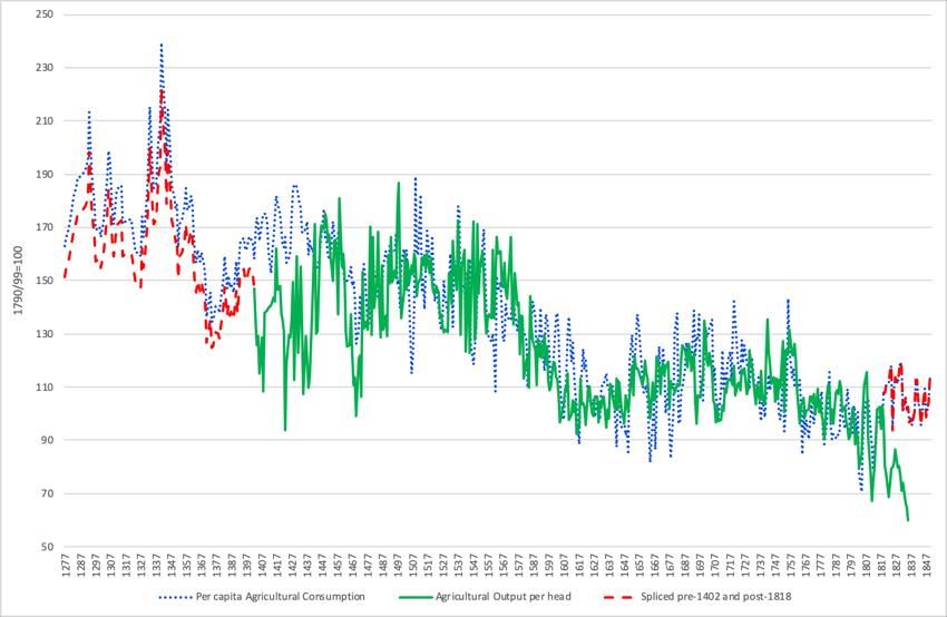
EHES Working Paper | No. 177 | March 2020
          Growth Recurring in Preindustrial Spain: Half a Millennium
                                Perspective*

                                 Leandro Prados de la Escosura1,
                                 Universidad Carlos III and CEPR

                                          Carlos Álvarez-Nogal2,
                                          Universidad Carlos III

                                      Carlos Santiago-Caballero3,
                                        Universidad Carlos III
       Abstract
       Research in economic history has lately challenged the Malthusian depiction of preindustrial
       European economies, highlighting ‘efflorescences’, ‘Smithian’ and ‘growth recurring’
       episodes. Do these defining concepts apply to preindustrial Spain? On the basis of new yearly
       estimates of output and population for nearly 600 years we show that preindustrial Spain was
       far from stagnant and phases of per capita growth and shrinkage alternated. Population and
       output per head evolved along supporting the hypothesis of a frontier economy. After a long
       phase of sustained and egalitarian growth, a collapse in the 1570s opened a new era of
       sluggish growth and high inequality. The unintended consequences of imperial ambitions in
       Europe on economic activity, rather than Malthusian forces, help to explain it.

       JEL Codes: E10, N13, O10, O47

       Keywords: Preindustrial Spain, Frontier economy, Black Death, Malthusian,
       Growth recurring

 * We are indebted to David Reher for his comments on the population section and to him and Enrique Llopis Agelán for
 sharing their dataset on baptisms
 1
   leandro.prados.delaescosura@uc3m.es
 2
   canogal@clio.uc3m.es
 3
   carlos.santiago@uc3m.es

                                                        Notice
 The material presented in the EHES Working Paper Series is property of the author(s) and should be quoted as such.
The views expressed in this Paper are those of the author(s) and do not necessarily represent the views of the EHES or
                                                     its members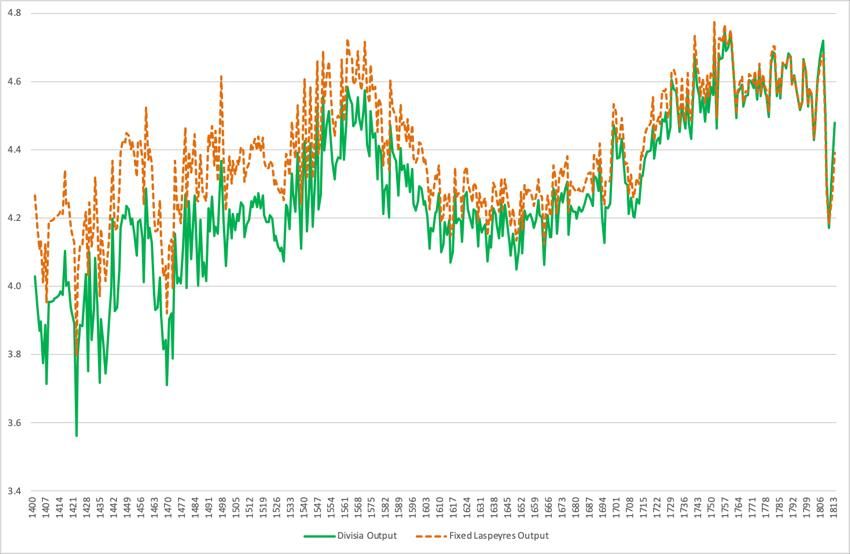
Prior to         living standards in world economies were roughly constant over
the very long run per capita wage income output and consumption did not grow
asserted Gary Hansen and Edward Prescott two decades ago.3 This stylised fact has
spread among economists in more simplified terms: human societies remained
stagnant in terms of income per person until the Industrial Revolution heralded the
beginning of modern economic growth. Such a perception has been reinforced by the
Unified Growth Theory s depiction of preindustrial societies as Malthusian (Galor and
Weil, 2000).4
        Although the Malthusian nature of preindustrial economies is defended by
distinguished scholars (cf. Clark, 2007, 2008; Madsen et al., 2019), research in
economic history has challenged it lately. Historians are now more prone to accept the
overcoming of the Malthusian constraint in preindustrial western Europe as capital
accumulation and productivity gains permitted higher population and income levels
simultaneously, but with the caveat that such achievements were limited in scope and
time (i.e., after the Black Death), and only had long term effects in the North Sea Area
(Pamuk, 2007). Broadberry et al. (2015) path-breaking research, for example, rejects
the term Malthusian to portray the early modern British economy.
        Furthermore, in an attempt to break the growth-stagnation dichotomy in
preindustrial societies, historians have highlighted efflorescences Goldstone
      and growth recurring episodes (Jones, 1988; Jerven, 2011) that feature a
succession of phases of growing and shrinking output per head and only give way to
modern economic growth when shrinking phases become less intense and frequent
(Broadberry and Wallis, 2017). Smithian growth, a process driven by gains from
specialisation resulting from the expansion of international and domestic markets,
may explain these episodes of sustained but reversible per capita income gains.5

3 Hansen and Prescott                 aimed at modelling the transition from stagnant to growing living
standards
4 That is, assuming a fixed supply of land and population growth as a response to an increase in living

standards.
5 Morgan Kelly (1997: 939-940), provides a suggestive explanation of Smithian growth based on the idea

of threshold behaviour Below a critical density of transport linkages the economy is split into small
markets with limited scope for division of labour. Once the critical density is reached, these small
markets begin to fuse together into large, economy-wide market. The resulting increase in specialisation
causes an acceleration in the growth rate

                                                   2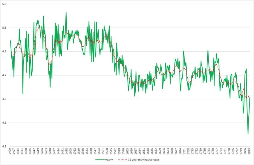
Did Smithian growth occur in preindustrial Europe beyond the North Sea Area?
New research suggests Iberia (Palma and Reis, 2019; Álvarez-Nogal and Prados de la
Escosura, 2013), although qualitative perceptions of early modern Spain as a stagnant
economy are deeply rooted (Kamen, 1978: 49; Cipolla, 1980: 250). In this paper an
effort is made to provide yearly estimates of Spanish output and population for more
than half a millennium. On the basis of new evidence on long-run economic
performance we discuss the extent to which Malthusian, efflorescences, growth
recurring, or Smithian growth are defining elements of preindustrial Spain.
       As basically a methodological and data paper, it includes sections presenting
controlled conjectures on population and sectoral and aggregate output estimates,
and a discussion of their trends in the context of the historical debate. A summary of
the results and a research agenda conclude the paper.
       Our main findings can be summarised as follows: 1) Preindustrial Spain s
economy was far from stagnant, exhibiting phases of output per head growth and
contraction. 2) As a result, the peak average income levels reached in the 1340s and
the 1570s were only overcome in the early nineteenth century. 3) Spain s performance
matches Smithian growth during the long rising phase up to the Black Death, the
century-long expansion up to the 1570s, and the sustained recovery from the late
seventeenth century to the Peninsular War (1808-1814), when larger markets
favoured specialization and urbanisation and promoted growth. 4) Population and
output per head evolved along, a finding that provides support for the hypothesis of
Spain as a frontier economy, and is at odds with the Malthusian narrative. 5) Why no
significant long-run gains in living standards were achieved in Spain s frontier
economy? In the absence of a persuasive Malthusian interpretation, an institutional
explanation deserves to be explored. It can be hypothesised that sustained increases in
fiscal pressure on dynamic urban activities to finance imperial wars in Europe triggered
de-urbanisation and led to a collapse in average real incomes, from which early
modern Spain never fully recovered. 6) Income was distributed in a rather egalitarian
way until the mid-sixteenth century, as would be expected in a frontier economy.
However, income distribution became increasingly unequal thereafter as the relative
importance of land as a production factor increased.

                                            3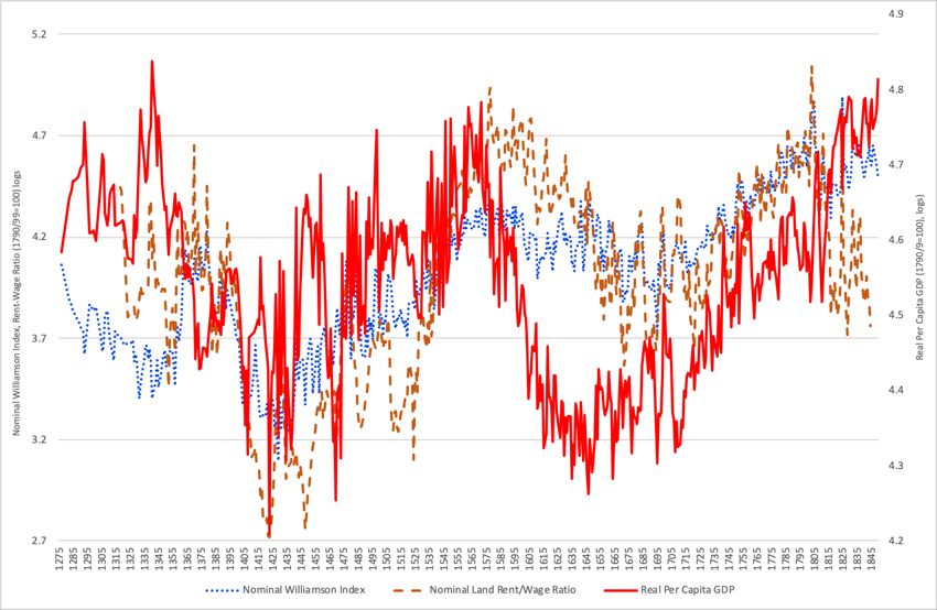
Population: Quantitative Conjectures
        Aggregate population figures for late medieval and early modern Spain consist
of scattered benchmark estimates from household population surveys usually
collected for taxation purposes, the so-called vecindarios (literally, neighbourhoods),
that present the challenge of converting households into inhabitants, national
censuses for the late eighteenth century, and sporadic assessments for the early
nineteenth century.6 Available benchmark estimates allow us, nonetheless, to derive
long run population trends. Moreover, historians have relied on baptism records to
represent population dynamics.7
        Baptism indices are yearly available for practically all regions between 1700 and
1809, although its coverage declines as one moves back to 1580 and from 1809
onwards.8 Thus, an annual national index can be derived by weighting each regional
index, Brt, expressed as 1790-99=1, by the average of regional population in 1787 and
1797 censuses, Nr1787-97 .9
                             B.t =   Nr1787-97 * Brt     for      t T            (1)
        Figure 1 presents annual population estimates derived from baptism indices
along those obtained through log-linear interpolation of each pair of adjacent
benchmark estimates.10 It can be observed that, from the early seventeenth to the late

6 Pre-1850 population estimates from household surveys and censuses are available for 1530, 1591,
1646, 1712-17, 1752, 1768, 1787, 1797, 1821, and 1833. Cf. Nadal (1984), Bustelo (1972, 1973, 1974),
Pérez Moreda (1988), and Reher (personal communication). For the conversion of households into
inhabitants, cf. Martín Galán (1985).
7 Cf. Nadal (1988), Reher (1991), Llopis Agelán (2004), and Llopis Agelán and Sebastián Amarillas (2007).
8 From 1700 onwards we used Llopis Agelán (personal communication), who kindly provided us with an

updated dataset, completed with Nadal (1988) for 1580-1700. In the case of New Castile we have
preferred Reher (1991) indices. For La Rioja, Gurría (2004) indices have been used. We assumed that
missing regions were represented by neighbour ones (see fn. 12).
9 As the regional coverage diminishes as we move back in time, we have constructed indices for each

regional sample and spliced them into a single index given preference to the indices with broader
regional coverage.
10 The benchmark levels used have been 1340, 1420, 1530, 1591, 1646, 1712-17, 1752, 1787, 1797,

1821, 1833, and 1850.The main source is Pérez Moreda (1988: 368, 372, 384-385, 402) who surveys
alternative estimates and conjectures. In the case of 1712-17, Pérez Moreda 1(988: 384), on the basis of
Bustelo (1973, 1974) provides a 7.7-8.15 million range. Here we have been accepted the lower figure,
7.7 million after Llopis Agelán (2002: 123), and attributed it to 1717. The figure for 1787, comes from
the census (Anes, 1975: 24) and that for 1850 from Prados de la Escosura (2017). The estimate for 1833
has been increased by 5% to offset its underestimate as Pérez Moreda (1988: 402) did for 1797. For
       and       we have assumed Portugal s population as 1.0 and 0.5 million that was subtracted from
the overall figure for Iberia (Pérez Moreda 1988: 368. His estimate for 1300 has been accepted for 1340
here. In order to allow for the Jew population expelled after 1492, we have accepted Pérez Moreda
(1988: 368) estimate of 150,000 people and distributed over 1493-1497, starting from an arbitrary

                                                    4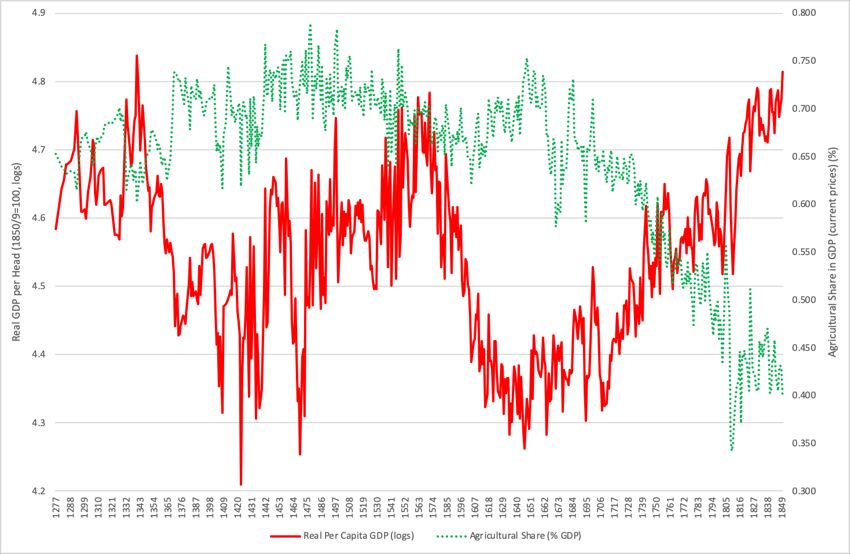
eighteenth century, the baptism-based series shadows the interpolated series but at a
lower level. It also reveals baptisms high volatility that precludes inferring yearly
population levels from it.11 Moreover, inferring population trends from baptisms
implies assuming that deaths rates kept a stable short-term relationship with birth
rates12 and net migration flows were negligible over time.13
        Since these assumptions are highly unrealistic, Álvarez-Nogal, Prados de la
Escosura, and Santiago-Caballero (2016) offered a compromise solution, namely,
reconciling population benchmarks with decadal estimates of baptisms, available since
the 1520s, so the resulting estimates capture migration (forced or voluntary) and over
time variations in the proportion between birth and death rates (and between births
and baptised children).
        Thus, in a first attempt to estimate total population for the post-1520 period,
we have followed this approach projecting each benchmark population estimate with
decadal baptism series back and forth.14 Since the projected benchmark levels with
baptism indices do not match the adjacent benchmark estimates, a variable-weighted

figure of 50,000 in 1493 and reducing it by 10, 000 each year. These figures should be, perhaps,
augmented to include Muslim emigration as a consequence of the conquest of the Nazri Kingdom of
Granada by the Catholic Kings in 1492.
11 Unless we assume an almost perpetual pandemic scenario with population varying by the hundred

thousand from one year to another!
12 Llopis Agelán (personal communication) discusses the relationship between deceases and baptisms

during the eighteenth century showing a 11 per cent decline in this ratio between its first and second
half that, however, does not seem attributable to a decline in infant mortality. This author also warns us
that the number of births exceeded that of baptised children and their proportion declined during the
eighteenth century, that he estimates in 5-6 per cent for Old and New Castile.
13 Some evidence exemplifies how misleading this assumption is. For example, the number of Moorish

expelled from Spain (1609-1613) could have reached 300,000 (Pérez Moreda 1988: 380). As regards
voluntary migration, flows to Spanish America have been estimated as 250,000 and 100,000 in the 16th
and 17th centuries, respectively, and about 125,000 over 1700-1824 (Martínez Shaw, 1994: 152, 167,
249).
14 Regional data on baptisms, expressed in index form, are available at decadal intervals for all Spanish

regions since 1700, with its regional coverage narrowing down as one moves back to the 1520s. For
1580s-1790s we used Llopis Agelán (personal communication) and Llopis Agelán and Sebastián Amarilla
        decadal regional estimates completed with Reher s for         s-1580s (personal communication).
Since the coverage for earlier decades declines, we assumed that some regions moved along its
neighbours, namely, Asturias presumably evolved as Galicia during 1610-30; Cantabria as the average of
Galicia and the Basque region, 1620-30; and Galicia, Asturias, and Cantabria as the Basque region over
1580-1610. Also, Valencia and Murcia were assumed to move with Catalonia during 1580-1600, and
with Balearics during 1580-1590. Regional coverage is restricted to the Kingdom of Castile and Navarre
for the 1580s as information is available neither for Catalonia, Valencia, and Balearics, nor for the
Canaries. Data for 1550-1580 are restricted to Castilla-León that was assumed to represent also the
evolution of northern Spain (Galicia, Asturias, Cantabria, and the Basque region), Castilla-La Mancha,
Madrid, and Extremadura (that was used to represent the evolution of Andalusia).

                                                    5
geometric average has been computed for each pair of estimates previously derived
using adjacent benchmarks, in which the closest benchmark series gets a larger weight.
Thus,
                    Nd = (Xd)(n-t)/n * (Yd) t/n         for     t T           (2)
          Being N the population at decadal estimates d, X and Y, the values
  corresponding to the projection of each adjacent benchmark (initial and final)
  figures (i.e., 1700 and 1750) with baptism decadal indices, respectively; and n the
  number of years in between 0 and T.

          It could be argued that a similar reconciliation is also possible between
  benchmark interpolated series and those obtained from baptism yearly indices that
  would result in new annual series from 1580 onwards. We have, thus, carried out
  this alternative estimate using the yearly baptism indices and the benchmarks in
  expression (2). The outcome is presented in Figure 2, along the benchmarks log-
  linearly interpolated and its adjustment with decadal indices of baptisms. However,
  the high volatility of the baptism-based yearly series renders them unacceptable.

          Unfortunately, this compromise solution is questionable. Projecting a
  population benchmark with baptism indices is misleading since population is a stock
  variable while baptism series, as a proxy for births, represent a flow. In fact, using
  baptisms as measure of population amounts to proxy capital stock by investment.

          Following this analogy, we could use the Perpetual Inventory Method to
  reconstruct population. Thus,

                                   Nt = (1 -      t)   Nt-1 + Bt + Mt   (3)

          Where population N in year t equals population in the year t-1 multiplied by
  1 minus the depreciation rate ( ) in year t, that here would be represented by the
  crude death rate, plus baptisms, B, as a proxy for the number of births, and net
  immigration, M, (that is, immigrants less emigrants) in the year t.

          Unfortunately, although baptisms would roughly amount to crude birth
  rates, cbr, times population at the beginning of the year, we lack yearly crude death
  rates, cdr, and any attempt to derive population by assuming fixed cdr is

                                                  6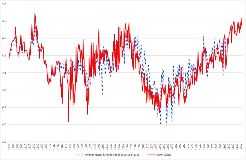
unacceptable as crude birth and death rates fluctuate widely in the short run, and
     even more at times of pandemics.

            Still, the ideal procedure to reconstruct annual population figures is to start
     from a reliable population figure at the beginning of a benchmark year adding up
     annually the natural increase in population, that is, births (bt) less deaths (dt), plus
     net immigration (mt).

            As there are population estimates available at various benchmarks (see
     footnote 5), all we need, then, is data on the natural increase in population (births
     less deaths) and net migration.

            On migration no yearly data are available and only crude estimates can be
     proposed. As regards emigration to the Americas we have relied on Morner (1975:
     64) who provides aggregate figures for five periods over 1506-1670 (1506-40, 1541-
     60, 1561-1600, 1601-25, 1626-50) and have distributed them annually within each
     period.15 We also allowed for the outflow of Moorish population after their
     expulsion, that Pérez Moreda (1988: 380), reckons in, at least, 0.3 million. Thus, we
     have added a figure of 60,000 emigrants for each year between 1609 and 1613
     inclusively. Estimates from 1670 onwards come from Martínez Shaw (1994: 151,
     167, 249) for the periods 1670-1700, 1700-1800, 1800-30, and 1830-50 that have
     been distributed annually. As regards immigration, a figure around 0.2 million has
     been estimated for the sixteenth century, mostly French moving to Catalonia (Pérez
     Moreda, 1988: 374), that we have distributed assuming a steady inflow of 2,000
     people per year.

            However, as already mentioned, we lack yearly crude birth and death rates
     for Spain prior to the 1850s. Fortunately, David Reher (1991) computed them
     annually for New Castile since 1565. Hence, a possibility to provide plausible
     conjectures on annual population levels consists of constructing alternative
     population estimates in which each population benchmark (Nbk) is projected forth
     by adding the annual natural increase in population derived from yearly crude birth

15Although Martínez Shaw         argues that Morner s figures for the early seventeenth century are
grossly overexaggerated, we have accepted them as a way to offset the population disappeared as a
consequence of war in Europe during the second quarter of the century.

                                                  7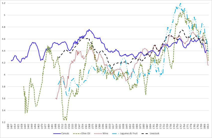
and death rates for New Castile (cbrnct and cdrnct), plus net immigration estimates.
      This is the procedure to operate when we move forward (that is, when starting in
      1787 we want to estimate population in 1788), while we need to subtract the
      natural increase in population and the net immigration in the previous year when
      we project population backwards (namely, when starting in 1787 we want to
      compute population in 1786).16 That is,

                       Nt+1 = Nbk + (cbrnct - cdrnct)*Nbk + mt               for t > bk   (4)
                       Nt-1 = Nbk - (cbrnct-1 - cdrnct-1)*Nbk - mt-1        for t < bk    (5)
           Accepting crude birth and death rates from New Castile assumes implicitly that
they are representative for the whole of Spain. Such arbitrary assumption is largely
relaxed by the procedure used to reconcile the resulting series. In fact, the exercise
suggested by expressions (4) and (5) provides a set of population series, one for each
benchmark, that do not match each other for the years in which they overlap (Figure
3). Therefore, we need to carry out a reconciliation between these alternative
estimates.
           A solution is interpolating the series accepting the levels for each benchmark-
year as the best possible estimates and distributing the gap or difference between
adjacent benchmark series (say, series obtained by projecting the 1752 benchmark
forward, N1752t, and the 1787 benchmark backwards, N1787t) in the overlapping year T
at a constant rate over the time span in between the two benchmark years.
                  NIt = N1752t * [(N1787T / N1752T)1/n]t         for     t T                    (6)
               Being NI the linearly interpolated new series, N1787t and N1752t the series
      pertaining to population obtained by projecting two adjacent population
      benchmarks (i.e., 1752 and 1787) with expressions (4) and (5), respectively; t, the
      year considered; T, the overlapping year between the two benchmarks series say
      1787); and n, the number of years in between the two benchmark dates (that is, 35
      years, 1787 less 1752, in our example).

               Alternatively, a variable-weighted geometric average for each pair of
      estimates derived using adjacent benchmarks, in which the closest benchmark
      series gets a larger weight, can be used (expression (2)). We have used both

16   This crude approach is inspired by the inverse and back projection (Lee, 1985)

                                                      8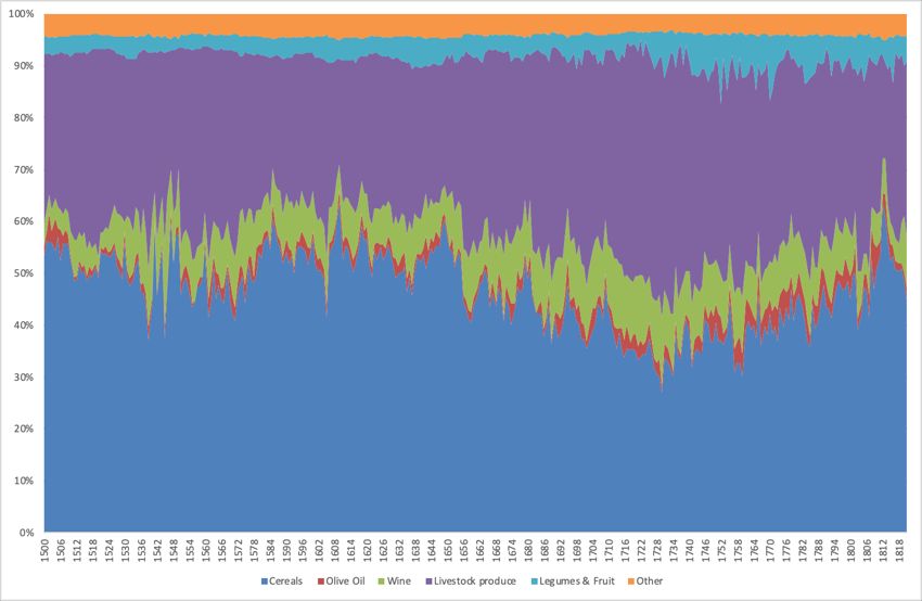
approaches with identical results but have kept the ones from the linear
     interpolation as this is the splicing procedure used in modern national accounts.

            Figure 4 presents the new compromise estimate along the decadal-adjusted
     series and the benchmarks interpolation. The comparison reveals that the main
     discrepancies correspond to the pre-1700 period, as the new compromise series
     continues expanding during the first quarter of the seventeenth century while the
     decadal-adjusted series peaks in the 1580 declining thereafter, and, especially, in
     the second half of the seventeenth century with deep contractions in the late
     1640s-early 1650s and in the mid-1680s. Also, the compromise series departs from
     the other two in the early nineteenth century capturing the impact of the
     demographic crisis in the early 1800s and during the Peninsular War.

         In Figure 5, we present our proposal about the evolution of Spanish population
that combines the compromise series since 1565 with the annual population figures
obtained through the decadal adjustment (with baptisms data) of the benchmarks
interpolated series for the period 1520-1565 and the benchmarks interpolated series
for the pre 1520 period.
Agricultural Output
         In preindustrial Europe, lack of data has led to estimate agricultural output
indirectly (Wrigley, 1985; Malanima, 2011; van Zanden and van Leeuwen, 2012). Using
a demand function approach, Álvarez-Nogal and Prados de la Escosura (2013)
computed agricultural consumption per head, and assuming the net imports of
foodstuffs were negligible, they used them to proxy output per head. 17 These findings
may be largely considered explicit conjectures as they are based upon limited
empirical evidence on real wage rates and land rents, used as proxies for disposable
income per head, and hypothetical values for income- and own price elasticities.
Exploring new indirect alternatives seems, hence, warranted while provides a test for
the robustness of the demand approach estimates.

17Real consumption per head of agricultural goods (C) can be expressed as
                                           C = a Pε Y Mγ      ([7].
In which P and M denote agricultural and non-agricultural prices relative to the consumer price index,
respectively; Y stands for real disposable income per head; ε, , and γ are the values of own price,
income and cross price elasticities, respectively; and a represents a constant.

                                                   9
Early modern economic historians have used indirect information on a religious
tax, the tithe, to infer trends in agricultural output. In Spanish economic history,
studies of main crops output using tithes date mostly from the s and early s
Monographs were mainly carried out at local or provincial level, although regional
studies have occasionally been carried out. A first attempt at assessing the evolution of
agricultural output in Spain on the basis of the tithe series was carried out by Gonzalo
Anes and Ángel García Sanz (1982). More recently, we used tithes to infer the
evolution of agricultural output in Spain between 1500 and 1800 (Álvarez-Nogal et al.,
2016). Here we improve these estimates and expand its time coverage.
Tithe records go back to the Middle Ages but the dearth of written sources
reduces the time span in which they are available. Tithes were imposed on farming
and livestock production and although, nominally, represented 10 per cent of total
production, in practice, its share fluctuated and was usually smaller.
In Spain, tithes can be traced back to the early fifteenth century for cereals and
olive oil and to the end of the century for wine, while for fruits and vegetables and
livestock tithes already exist for the sixteenth century. In Roman Catholic countries
tithes did not disappear until the French Revolution and the Napoleonic Wars. In the
case of Spain, tithes persisted until the 1830s (Canales, 1982), but its reliability to
capture output tendencies after 1808 is hampered by lack of compliance as a result of
the Peninsular War and the institutional collapse of the Ancien Régime.
The translation of tithes into output trends raises some questions. Collection
procedures, whether direct or rented out to private agents, and the payment system
(in kind or cash) changed over time and varied across regions. Also, the resistance of
peasants to pay the tax varied, as did the tax exemptions of specific producers, and the
opportunities for evasion resulting from the emergence of new crops. Does all this
render tithes questionable as a proxy for output tendencies?
In favour of the use of tithes it can be asserted, though, that in late medieval
and early modern Spain, where different fiscal systems operated, tithes provided
homogeneous information across regions. Moreover, tithes were computed on total
output, with the local priest acting as supervisor and making public the names and
amounts paid by each producer. The latter also found in its publicity a guarantee of
property rights on the harvested land (Santiago-Caballero, 2011, 2014). Lastly, the
10diversity of tithe beneficiaries multiplied the accounting records available allowing a
direct comparison between alternative sources. All this has led historians to depict
tithes as a fixed proportion of total production from which output trends can be
inferred (García Sanz, 1979).
Figure 6 presents output for the main crops that exhibit highly coincidental
trends (See Appendix 1 for its construction on the basis of tithes). Cereals show a long
run expansion up to the 1570s. Wine and livestock produce, especially, shadow cereals
tendencies. Wine production expanded remarkably during the first two-thirds of the
sixteenth century, remaining at high output levels until 1590. This depiction also fits
olive oil, a more volatile product. Most crops fell, then, during the early seventeenth
century recovering, at different pace, between the mid-seventeenth and the mid-
eighteenth centuries. In the late eighteenth century, opposite trends are found: fruits
and legumes and olive oil sustained declined while cereals, must, and livestock
produce expanded. A fall is observed across the board in the early nineteenth century.
In order to construct an index of agricultural output, one option is weighting
the quantity index for each crop by its share in 1799 agricultural output. However,
using fixed weights over such long time span introduces a serious index number
problem, since relative prices change over time and, consequently, 1799 weights
become less representative as one moves away from the late-eighteenth century.
A better choice seems to construct a Divisia index of agricultural output which
is obtained by weighting yearly variations in each crop s output by the average in
adjacent years, of the shares of each crop in agriculture output at current prices and,
then, obtaining its exponential. That is,
lnQat lnQat-1 = Σi Qit (lnQit - lnQit-1)] (8)
Where share values are computed as:
Qit it it-1)] (9)
Previously, current values, V, for each crop i at year t can be derived by
projecting the value of each crop in 1799, Vi1799, backwards with the quantity index
built on the basis of tithes, Q, and a price index, P (expressed as 1790/99 = 1) and then,
added up in order to obtain the value of total agricultural output, Vj.
Vat ΣVit ΣVi1799 * Qit * Pijt [10]
11Later, the share of each crop, Vit/Vt, needs to be obtained.18
The share of each major crop in agriculture output at current prices is
presented in Figure 7. It can be observed that cereal and animal produce are the main
contributors to agricultural output and show opposite trends, with animal produce
increasing its share and cereals share declining up to the 1570s and in the late
seventeenth and early eighteenth century and cereals share expanding at the
expense of animal produce s in the early seventeenth and late eighteenth century
Figure 8 offers the evolution of aggregate agricultural output obtained
computed both as Divisia and Laspeyres (with fixed 1799 weights) indices, that shadow
each other, although the Laspeyres index exhibits increasingly higher levels as ones
moves back time. This widening differential evidences the extent of the index number
problem triggered by keeping fixed weights over time.
In the evolution of agricultural output, distinctive phases can be found. The first
one was of sustained expansion that peaked in the early 1560s. A contraction occurred
between the mid-1570s and the early 1600s followed, then, by stagnation. A long-run
expansion took place from the mid-seventeenth to the mid-eighteenth century,
peaking in the 1750s, when the highest output level in four centuries was reached.
Output stabilised, then, until the end of the century and declined during the Peninsular
War.
If we focus now on agricultural output per person (Figure 9), two main phases
can be noticed, a high plateau covering from the 1440s to early 1570s, and a low
plateau spanning between the 1650s and the 1750s, with a transitional phase of
decline, between the late 1570s and the 1640s, in between, in which output per
person shrank by one-third. A new phase of contraction is found in the late eighteenth
century that reached its trough during the Peninsular War and represented one-fourth
contraction since the 1750s.
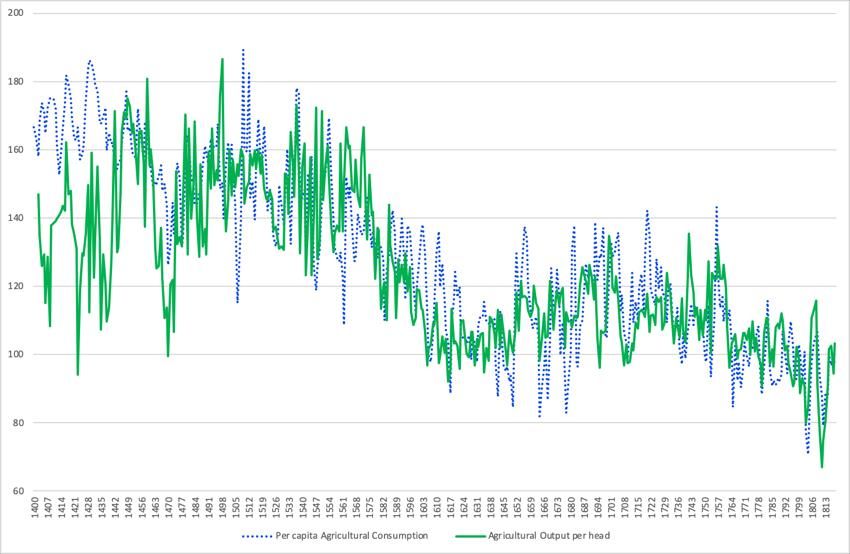
How does the new tithes-based agricultural output per head compare to the
earlier demand function estimates? Both series present roughly the same trends since
the mid-fifteenth century, but while the demand approach series were already on high
plateau since 1400 the tithes-based series showed lower levels and higher volatility up
18 See the sources of agricultural prices in Appendix 2.
12to the 1440s (Figure 10). The shift from a high to a low path of output per head is
common to both estimates, which reach a trough in the early seventeenth century,
although the tithes-based series present a sharper and neater decline, starting in the
mid- late 1570s, rather than in the 1560s. The lower plateau covers the same period,
1650s-1750s, in the two set of estimates, but in the tithes-based ones the post-1650
recovery is stronger and exhibits less volatility. After 1800 the two series evolve
alongside but the tithes-based shows stronger fluctuations.
It is worth noting that the parallel behaviour of the demand-approach and
tithes-based series supports the view that crop and livestock destruction appears as
the main factor behind the sharp decline in tithes collection during the Peninsular War,
rather than the more intuitive view of peasants lack of compliance with the religious
tax.
Further support to this interpretation is obtained when we extend the
comparison between the two alternative approaches to the early 1830s. Although
both goods and regional coverage narrows down for the early nineteenth century, it is
still possible to construct indices of agricultural output on the basis of tithes until 1835.
Figure 11 shows how the tithes-based output departs sharply from output derived
with the demand approach from 1820 onwards. The fact that the years between 1820
and 1833 correspond to a period of peace, suggests that it is non-compliance with the
religious tax the reason why a growing gap emerges between the two indices. The so-
called Trienio Liberal (1820-23), a phase of liberalisation, weakened Ancien Régime
institutions and discouraged tithe compliance (Anes and García Sanz, 1982; Canales,
1982; Torras, 1976). The bottom line is, therefore, that the parallel trends of the tithe-
based and the demand approach estimates supports the use of tithes as a reliable
indicator of agricultural output tendencies until 1818 or, to be on the safe side, until
the end of the Peninsular War (1814). Moreover, our findings challenge the dismissal
of the demand approach as simple controlled conjectures. Lacking direct sources of
agricultural production, as it is often the case in preindustrial societies, the demand
approach appears to provide a reasonable procedure to infer output trends.
Since our goal here is to provide the best possible estimate for long run
agricultural output, we propose a new index that accepts the demand approach
13estimates for 1818-1850 and the tithe-based ones for 1402-1818, and projects its level
for 1402 back to 1277 with the demand approach index (red dash line in Figure 11).
Output in Non-Agricultural Activities: Urbanization as a Proxy
A reconstruction of trends in industrial and services output is beyond the scope
of this paper. It would require a thorough investigation of industrial output, sector by
sector, most probably on the basis of a variety of indirect indicators among which
taxes deserve to be explored. In the case of services, the prospects to get a proper
assessment of output are even bleaker. A crude short cut to proxy trends in economic
activity outside agriculture is urbanization, more specifically, the use of changes in the
urbanization rate (ratio between urban and total population) to infer trends in non-
agricultural output per head.19
The association between urbanization and the expansion of modern industry
and services is not new. Simon Kuznets (1966: 271) observed that urbanization implies
an increasing division of labor within the country growing specialization and the shift
of many activities from nonmarket-oriented pursuit within the family or the village to
specialized market-oriented business firms In the economic history literature
parallels have been drawn suggested between changes in urbanization rates and per
capita income (Acemoglu et al., 2005; Craig and Fisher, 2000; Temin, 2006; and van
Zanden, 2001). Wrigley has argued A rising level of real income per head
and a rising population of urban dwellers, other things being equal, are likely to be
linked phenomena in a preindustrial economy
Although keeping a constant threshold over time, while population grows, is
rather questionable (Wrigley, 1985: 124), we have arbitrarily adopted the definition of
urban population as dwellers in towns of 5,000 inhabitants or more.20 Indeed, this
measure provides a lower bound of the actual level of urbanization as it does not take
into account the increase in population living in towns and cities of larger size.
However, a caveat is necessary. Urban population has been accepted here as a
proxy for output in non-agricultural activities after excluding those living on
19 We follow here Álvarez-Nogal and Prados de la Escosura (2007, 2013). Malanima (2011) also relies on
urbanization as a proxy for non-agricultural economic activity.
20 This way, we maintain consistency with Bairoch et al. (1988) large database facilitating international
comparisons. Alternative thresholds of 10,000 (de Vries, 1984) and 20,000 inhabitants have been used
(Flora, 1981). Bairoch et al. (1988) employed alternatively 2,000, 5,000, 10,000, and 20,000 inhabitants.
14agriculture The reason is that the existence of agro-towns namely towns in which a
sizable share of the population was dependent on agriculture for living) appears to be
a feature of pre-industrial Spain. Thus, we have computed trends in the rate of
adjusted urbanization -that is, the share of non-agricultural urban population in total
population- in an attempt to capture those in industry and services output per head
(See a detailed explanation of the computing procedure in Appendix 3).21
Agro-towns sink their roots in the Reconquest. In a frontier economy, towns
provided security and lower transactions costs during the re-population following the
southwards advance (Ladero Quesada, 1981; Rodríguez Molina, 1978). In the
thirteenth century, Christian settlers from Aragon, Catalonia, and Southern France
acquired farms but preferred to live in towns (MacKay, 1977: 69). It has been claimed
that in southern Spain agro-towns were the legacy of highly concentrated
landownership after the acceleration in the pace of the Reconquest and the Black
Death, which increased the proportion of landless agricultural workers (Vaca
Lorenzo,1983; Valdeón Baruque, 1966), although Cabrera (1989) attributes the rise of
latifundia to the generalization of the seigniorial regime during the fourteenth and
fifteenth centuries. In our estimates, agro-towns appear mainly located in Andalusia
and since the late eighteenth century, also in Murcia and Valencia.
Albeit the existence of agro-towns urban economic activity was closely
associated to industry and services. In sixteenth century Old Castile, Yun-Casalilla
(2004) reckons, only one in twelve in the urban labour force worked in agriculture.
Pérez Moreda and Reher (2003: 129) suggest, for 1787, a similar proportion of farmers
in Spain s urban population 22
Moreover, rural population carried out non-agricultural activities (storage,
transportation, domestic service, construction, light manufacturing) especially during
21 In order to mitigate the inclusion of agro-towns Malanima proposed for the south of Italy a
limit of 10,000 inhabitants for being considered urban, as opposed to the 5,000 inhabitants limit for the
north and centre of Italy. Cf. Llopis Agelán and González Mariscal (2006) for a more astringent definition
of urban centre
22 However, Reher (1990) reckoned half the economically active population living in towns in Spain
worked in agriculture by Nonetheless Reher s computations are on the high side as he increased
artificially the share of urban population employed in agriculture by allocating all day labourers to this
sector while excluding servants from the labour force.
15the slack season in agriculture (Herr, 1989, López-Salazar, 1986).23 Perhaps, as Wrigley
(1985: 137) noted, a more rigorous option would be to measure employment
composition by sector in terms of days or hours worked, rather than assigning each
worker to a specific occupation. 24
Table 1. Urbanization Rates, 1340-1857: Benchmark Estimates (%)
Unadjusted ‘Adjusted
1340 (11.6) (9.2)
1420 (9.4) (7.5)
1530 12.0 9.5
1561 18.9 13.0
1591 20.5 14.6
1646 8.7 8.7
1700 10.0 9.9
1750 14.6 13.8
1787 24.6 17.4
1857 31.4 22.9
Sources: Total urban population, Bairoch et al. (1988), Correas (1988), and Fortea (1995); for non-
agricultural urban population, see Appendix. For absolute population, see the population section.
Note: Figures in brackets are highly conjectural.
Spanish urban population, adjusted to exclude population living on agriculture,
has been computed at benchmark years for the period 1530-1857. Total and adjusted
urban population levels for 1530 were projected backwards to 1300 and 1400 with
Bairoch et al. (1988: 15-21) estimates. Urban population for Spain in, 1530, 1561, and
1646 has been inferred from data for the Kingdom of Castile. Urbanization rates, that
is, urban population expressed as a share of total population, both unadjusted and
adjusted are presented at benchmark years in Table
Annual adjusted urbanization rates have been derived through linear
interpolation of the benchmark estimates. Trends in the rate of urbanization are
shown in Figure 12. The accelerated expansion of the early sixteenth century slowed
down in its second half and was reversed during the first half of the seventeenth
century. Then, urbanization recovered slowly accelerating after the Succession War to
overcome the late sixteenth century peak by the second half of the eighteenth
23 Wool provides a case in point in early modern Spain. A mainly rural activity, it had both industrial and
services (trade, transport, financial services) dimensions (García Sanz, 1986).
24 The number of days (and hours) worked per EAP in Spain was lower in agriculture than in industry and
services leaving extra time to work in non-agricultural activities. Cf. Santaolaya (1991), Vilar (1970: 19),
and Ringrose (1983).
16century. Interestingly, these figures are at odds with the rather stable rate of
urbanization (around 20%) widely used estimates by Bairoch et al. (1988).
Aggregate Output
The next stage is to construct an index of aggregate output (Q). Rather than
estimating long-run output with fixed weights which introduces an index number
problem, as implicitly assumes that relative prices do not change over time, we have
computed a Divisia index in which real GDP is obtained by weighting yearly output
variations in agriculture, Qat, and industry and services, proxied by adjusted urban
population, N´urb-nonagr t, with the average, in adjacent years, of the shares of
agriculture, Qat, and non-agricultural activities, Qi+st, in GDP at current prices.25 That
is,
lnQt lnQt-1 = Qat (lnQat lnQat-1 Qi+st (lnN´urb-nonagr t - lnN´urb-nonagr t-1) (11)
where agricultural, Qat, and non-agricultural, Qi+st, share values are computed as:
Qat at at-1 and Qi+st i+st i+st-1)] (12)
and, then, Qt is obtained as its exponential.
In order to get sector shares in current GDP it, current values, V, for each
sector i at year t are derived by projecting each sector s value added average in
1850/9, Vi1850/9, backwards with the quantity, Q, and price P, indices previously built for
each sector, Qat and Pat for agriculture, and N´urb-nonagr t adjusted urban population
and Pi+st, for industry and services, respectively, (expressed as 1850/9 = 1) and, then,
added up to attain the value of total output, V.t
Vat = Va1850/9 Qat Pat (13)
Vi+st = Vi+s1850/9 N´urb-nonagr t Pi+st (14)
V.t = Vat + Vi+st (15)
Later, the shares of agricultural and non-agricultural activities were obtained,
respectively, as Qat = Vat/Vt. and Qi+st = Vi+st/Vt
As regards price indices, the price index already built in the section on
agriculture has been accepted. For non-agricultural activities an unweighted Divisia
25In the case of agriculture, note, as discussed in the section on agriculture, real output estimates with
the demand approach (Álvarez-Nogal and Prados de la Escosura, 2013) have been used for 1818-1850
and, then, spliced to the tithes-based index back to 1402 and, then, backwards projected to 1277 with
the demand approach index. As regards non-agricultural output the adjusted index of urban
population, that is the adjusted urbanization rate times population has been accepted to represent it
17index was computed with industrial goods and consumer price indices and nominal
wages.26 This amounts to allocating one-third of the weight to industry (the industrial
price index) and two-thirds to services (nominal wage and consumer price indices),
which represents a good approximation to these sector shares in non-agricultural
output in the 1850s (Prados de la Escosura, 2017) (For the source of prices see
Appendix 2).
Figure 13 offers the evolution of aggregate output obtained computed as
Divisia index along a Laspeyres index with fixed 1850/59 weights.27 It can be observed
that they match each other closely. Does this indicate lack of structural change in
preindustrial Spain? We will address this issue later.
The new output index provides a proxy for the evolution of real GDP in the
absence of direct alternatives. This approach has been deemed a reasonable second
best (Fouquet and Broadberry, 2015). But how robust are these results? A possible test
could be to consider an alternative scenario of three, rather than two, economic
sectors agriculture industry and modern or market services and traditional or
mainly non-market services, the latter including government, health, education,
leisure, professional and domestic services. It could be further hypothesised that
lacking data on the output of non-market services its evolution could be proxied by
that of population, under the plausible assumption that its labour productivity was
largely stable over time.28
Thus, we have constructed an alternative output index with three sectors,
agriculture industry and market services proxied by adjusted urban population and
non-market services (proxied by population) which represented 40.6, 27.8, and 14.5
per cent of GDP in the 1850s, respectively. The deflators used for industry and the rest
of services would be the same as the ones employed for non-agricultural activity in the
baseline output estimates, while for non-market services the price index used is a
26 Thus, average rates of variation for manufacturing prices, the CPI, and nominal wage rates were
arithmetically averaged and the price index obtained as its exponential.
27 That is, Q = S * Q /Q + (1 S )* N´
.t a0 at a0 a0 urb-nonagr t /N´urb-nonagr 0 (16)
where fixed 1850/59 shares for agriculture (Sa0) and non-agricultural activities (1 - Sa0) in GDP are used
as weights. Cf. Álvarez-Nogal and Prados de la Escosura (2007).
28 This assumption has led researchers to proxy the evolution of output in traditional or non-market
services by the number of people they employ or, lacking such information, by population (Cf.
Broadberry et al., 2015; Prados de la Escosura, 2012).
18weighted average of the consumer price index (2/3) and the nominal wage rate in
index form (1/3). Output has been derived using a Divisia index as for the baseline
index. Figure 14 offers the alternative indices. It can be observed that they show the
same trends although softened during growing and shrinking phases in the case of the
three-sector index as would be expected when an economic sector s output is proxied
by population. This result suggests that the baseline index can be deemed a
satisfactory proxy for the evolution of real output over time.
What does the long run evolution of output show? Distinctive phases can be
distinguished (Figure 15). Three phases of expansion: 1) up to the 1340s, whose
origins, we can conjecture, go as far back as to the mid-eleventh century; 2) from the
early fifteenth century to the early 1570s, more intense during the central decades of
the sixteenth century; and 3) from the mid-seventeenth to mid-nineteenth century,
punctuated by the Succession (1701-13) and Peninsular (1808-14) Wars. Two phases of
sustained decline complete the picture, the first one, triggered by the Black Death
(1348), very intense until the 1370s, that lasted until the early fifteenth century; and a
second one, from the late sixteenth to the mid-seventeenth century.
If we now turn to output per head (Figure 16), its evolution follows a wide W
shape, with phases of growth which peak in 1341, 1572, and 1850, separated by deep
contractions in the late fourteenth and early seventeenth century. Each phase of
expansion (1277-1341, 1374-1572, and 1647-1814) shows similar pace but, as output
per head declined sharply during shrinking episodes, each subsequent growth phase
starts from a lower level and, hence, evolves along a lower path, with the results that
per capita income levels hardly changed over the long run (Table 2). Nonetheless, in
terms of average income levels, we can distinguish a relatively high plateau from the
late thirteenth to the late sixteenth century, but for the Black Death and its aftermath,
and a low plateau that covered the seventeenth and early eighteenth century.
Table 2 offers yearly rates of variation for population and absolute and per
capita output. Panel A provides, from the second row onwards, growth rates between
peaks and troughs, while Panel B presents a breakdown of expansion and contraction
phases. We can observe that the shrinkage in the third-fourth of the fourteenth
century is comparable in intensity to that of the late sixteen century. The results
confirm the view that output per head and population evolved alongside, accelerating
19and declining simultaneously. In phases of expansion, population grew albeit output
responded more than proportionally, while in phases of contraction, population
growth slowed down turning negative in the third quarter of the fourteenth century
and the first half of seventeenth century. The early nineteenth century appears as a
distinctive period with population increasing at about twice the pace in previous
expansion phases, and per capita income growing faster too (0.5 per cent).
Table 2. Output and Population Growth, 1277-1850 (%)*
Output Population Output per head
Panel A
1277-1850 0.26 0.22 0.04
1277-1341 0.47 0.07 0.41
1341-1374 -1.39 -0.15 -1.24
1374-1572 0.37 0.19 0.18
1572-1647 -0.62 0.07 -0.69
1647-1814 0.50 0.27 0.23
1814-1850 1.45 0.96 0.49
Panel B
1374-1572
1374-1474 0.20 0.04 0.15
1474-1517 0.28 0.17 0.12
1517-1572 0.77 0.48 0.27
1572-1647
1572-1605 -0.96 0.24 -1.19
1605-1647 -0.36 -0.05 -0.30
1647-1814
1647-1714 0.37 0.17 0.21
1714-1808 0.70 0.36 0.34
1808-1814 -1.23 0.06 -1.29
Sources: See the text.
Note: * annual average logarithmic rates. The periodization corresponds to that of output per head.
How does the new index of output per head compare to earlier estimates by
Álvarez-Nogal and Prados de la Escosura (2013)?29 In Figure 17 the two estimates are
presented alongside. The new series appears more volatile in the fifteenth century, a
fact that could be attributable to the lower coverage of tithe-based agricultural index
29Álvarez-Nogal and Prados de la Escosura (2013) also computed a Divisia index of output per head,
using the adjusted urbanization rate as a proxy for non-agricultural activities per person but derived
consumption per head of foodstuffs with a demand approach from which agricultural output per head
was inferred.
20in terms of geographical and output composition. Moreover, in the new series the
economic collapse in the late sixteenth century began earlier (in the late 1570s, rather
than in the late 1590s) and was deeper. On the whole, the two estimates show a high
degree of coincidence in the period 1402-1818, when they alternative used tithes and
the demand approach to derive agricultural output.
Are there any lessons to be drawn from preindustrial Spain s experience Some
stylised facts about preindustrial societies can be perhaps put to the test. A first one is
that of long run stagnation in average incomes. The expansive and contracting phases
in the W-shaped evolution of Spain s real output per head contradict this widespread
view, even though living standards did not experience an improvement over the very
long run. These results lend support instead to the idea of growth recurring over six
centuries. Furthermore, Broadberry and Wallis (2017) claim that, as shrinking phases
become shorter and less frequent after growing phases, modern economic growth
emerges is confirmed by Spain s early nineteenth century experience Figure
A second stylised fact is the Malthusian nature of preindustrial economies.
Trends in Spanish population and per capita income, expressed in logs, are offered
alongside in Figure 18.30 A direct association seems to exist between population and
per capita income trends. Population and real output per head expanded
simultaneously up to the Black Death, during the late fifteenth and most of the
sixteenth century, and from the late seventeenth to the early nineteenth century;
conversely, population and income per person shrank in the late fourteenth and early
fifteenth century and in the early seventeenth century. How can we explain these
results at odds with the Malthusian view? The existence of a frontier economy,
resource abundant, in preindustrial Spain provides an answer. Given low population
density and high land-labour ratios, demographic expansion appears to have had
increasing economic returns in a largely pastoral society that was led by urban nuclei
and connected to international trade networks. The frontier economy helps to explain
why the Black Death had devastating economic effects despite its comparatively
milder demographic impact, as the Plague destroyed a pre-existing fragile equilibrium
(Álvarez-Nogal and Prados de la Escosura, 2013). Furthermore, why the Black Death
30
The logarithmic transformation makes trends clearer as the slope of the curves provide the pace at
which growth or decline occurred.
21did not represent in Spain the watershed it constituted in Carolingian Europe and the
British Isles may be explained by its specific traits. In western Europe, by wiping out
between one-half and one-third of the population, the Black Death reduced
demographic pressure on resources, raised land- and capital-labour ratios, and led to
higher returns to labour vis-à-vis land or capital and higher relative prices for non-
agricultural goods. Cheaper capital and labour scarcity led to lower interest rates and
higher wages that incentivised physical and human capital accumulation and
stimulated labour saving technical innovation and female participation (Pamuk, 2007).
The fact that factor proportions in post-Plague western Europe were similar to those
already existing in pre-Plague Spain contribute to explain why the negative
consequences of the Black Death prevailed in the late fourteenth and early fifteenth
century Spain.
Another stylised fact is the absence of structural change in preindustrial
economies. Was this the case of Spain? We have already noticed that real output
trends are hardly altered if derived as a Laspeyres or as a Divisia index, and such
coincidence suggests a positive answer to the question. But before jumping to
conclusions, let us take a glance at the share of agriculture in GDP (Figure 19). The
agricultural share represented two-thirds of GDP in the pre-Black Death era and
expanded to represent about three-fourths in the late fifteenth century, as the role of
towns and commerce in economic activity declined. Then, the expansion of industry
and services accounted for its mild contraction throughout the sixteenth century. After
the agricultural collapse since the late s ruralisation helps to explain why the
agricultural share increased up to three-fourths of GDP in the mid-seventeenth
century. Steady decline of the agricultural share took place throughout the eighteenth
century shrinking to less than half the value of GDP in the early nineteenth century.
Moreover, output diversification, evidenced by the expansion of wine, olive oil, and
fruits and legumes, during periods of per capita income growth, also suggests
structural change within agriculture.
An interesting contrast appears between two periods of economic expansion
and similar average incomes: the central decades of the sixteenth century present a
high agricultural share, while a much lower one is observed in the late eighteenth and
early nineteenth century. A decline in the share of GDP accruing to agriculture is
22usually taken as an indicator of structural change, so how can we explain the relatively
high share in the sixteenth century? It can be hypothesised that the source of the
demand pull may matter In the sixteenth century a thriving urban economy in Spain s
interior triggered the expansion and commercial orientation of agriculture, that
included livestock -merino sheep, in particular-. Rising population and living standards
demanded land to produce more agriculture goods and high-quality wool to be
exported to North-western Europe. In the late eighteenth and early nineteenth
century the pull of demand came not from the interior (with the exception of Madrid)
but mainly from towns in the periphery. Lower market integration between the
interior and the periphery, largely due to transport difficulties, helps to explain a
weaker agricultural response, with the demand for grain in coastal areas met by
imports rather than by domestic production from the interior as it had happened in
the sixteenth century (Cermeño and Santiago-Caballero, forthcoming). Therefore, we
can posit that some degree of structural transformation occurred in the Spanish
economy during expansive phases of growth recurring.
Spain s long run performance has been presented so far in average terms but
how were the gains and losses over successive growing and shrinking phases of per
capita income distributed among social groups? Was Spain a highly unequal society, as
is often assumed in the literature on preindustrial societies? Two alternative indicators
allow us to provide crude trends in income distribution. The Williamson Index, defined
here as the nominal (that is, current price) ratio between output per head and
unskilled wage rates and expressed with 1790/99=100, permits to draw trends in
inequality. The rationale underlying the Williamson Index is that GDP captures the
returns to all factors of production while the unskilled wage captures only the returns
accruing to factor, raw labour. Ideally one would require GDP and wage dividing by per
hour worked in order to normalise them, so our comparison of output per person and
wage rates provides a crude metric that may distort inequality tendencies. 31 This way,
average returns are compared with returns to unskilled labourers, that is, those at the
middle of distribution are compared with those at the bottom. We cannot say,
however, how close to the absolute poverty line unskilled wages are, although
31However, carrying out the comparison in current prices avoids the distortion introduced by the use of
different deflators for output and wages.
23You can also read