Master s Thesis-master in Energy Sciences-Offshore wind energy cost trends and learning curves - Gomez Tuya, N. (Nilo) () ...

Master´s Thesis- master in Energy
Sciences- Offshore wind energy cost
 trends and learning curves.

 Gomez Tuya, N. (Nilo) (n.gomeztuya@uu.nl)

 Supervisor: Atse Lowen

P a g e 1 | 65

Abstract

 This thesis aims to give an insight in the historic cost trends and developments of
offshore wind energy in the main five countries deploying this technology Europe. It has been
done by analysing 86 operational offshore wind farms commissioned after 2000 till the ones
under development that will be ready before the end of 2022. A first increase of the Capital
Expenditures (CAPEX) is found that is linked to various factors like the distance to shore and
depth, commodity prices and supply chain development till around 2015 when the cost starts
decreasing. Analysis’ results indicate that this late cost improvement may continue in the coming
years and it is caused by an amalgam of factors. Using CAPEX, Annual Energy Production,
Weighed Average Cost of Capital and Operational Expenditures, the development of average
Levelized Cost of Electricity (LCoE) is shown to increase also in the first period from 120 €/MWh
in 2000 towards 190 €/MWh in 2015 and then decreasing till 100 in the end of 2018, which is a
direct result of the CAPEX decrease and the effort into improve the efficiency. The results
indicate a learning in the last years that is expected to keep going in the near future, reaching
values of 2.5-2 €/MW for the CAPEX and around 50€/MWh for the LCoE.

 P a g e 2 | 65

Acknowledgement

 This thesis is submitted as part of the Master of Energy Sciences degree at the Utrecht
University. Elaborate this thesis has enriched my knowledge about offshore wind energy and
has encouraged me into develop this knowledge further in my life. I want to express my
gratefulness to everybody who supported me, helped me and contributed to the fulfilment of
this thesis. First of all, my family, that from Spain is still supporting me and friends for their
support and patience throughout this thesis. My sincere gratitude goes to my supervisor Atse
Lowen for his help and guide and also to Martin Junginger for his advice and critical view. I want
to thank Jose Carlos Palomar from MTorres for his time to help with the development of this
work and to Lucas Gonzalez Madruga from Vestas for his expert advice.

 P a g e 3 | 65

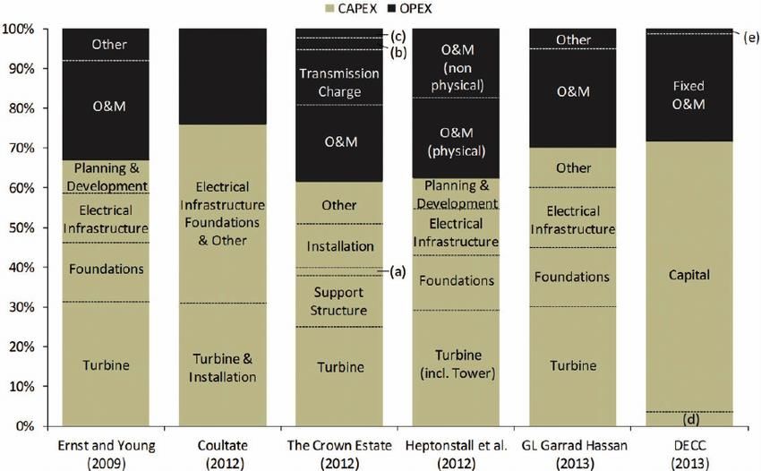
Table of contents

Abstract ......................................................................................................................................... 2

Acknowledgement........................................................................................................................ 3

Introduction .................................................................................................................................. 8

 Research questions ................................................................................................................. 13
Theoretical background .............................................................................................................. 14

 Offshore Wind Energy ............................................................................................................. 14
 CAPEX .................................................................................................................................. 15
 OPEX .................................................................................................................................... 16
 AEP ...................................................................................................................................... 16
 WACC................................................................................................................................... 16
 Levelized cost of Electricity ..................................................................................................... 18
 Experience and learning curves .............................................................................................. 19
Definitions and scope .................................................................................................................. 22

 Current situation ..................................................................................................................... 22
 Size and rated power........................................................................................................... 23
 Depth and distance from shore .......................................................................................... 24
Methods ...................................................................................................................................... 26

 Cumulative installed capacity and energy generation ............................................................ 28
 Calculating the LCoE ................................................................................................................ 28
 OPEX approximation ........................................................................................................... 28
 CAPEX calculation ................................................................................................................ 30
 WACC approximation .......................................................................................................... 30
 AEP calculation .................................................................................................................... 30
 Data harmonization................................................................................................................. 31
 Experience curves ................................................................................................................... 31
Results ......................................................................................................................................... 33

 Size, rated power and Capacity factor developments ............................................................ 33
 Distance and depth developments ......................................................................................... 34
 CAPEX developments .............................................................................................................. 35
 LCoE development .................................................................................................................. 39
 WACC results ....................................................................................................................... 39

 P a g e 4 | 65

Experience curves ................................................................................................................... 44
 One and Two factors experience curves ............................................................................. 45
 Expected development for 2030 ............................................................................................. 48
Discussion .................................................................................................................................... 51

Conclusion ................................................................................................................................... 53

Glossary ....................................................................................................................................... 55

Bibliography ................................................................................................................................ 56

Annex ............................................................................................................................................ 0

 P a g e 5 | 65

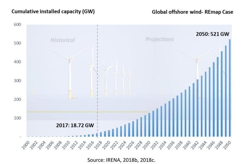
List of equations:

Equation 1: WACC calculation ..................................................................................................... 17
Equation 2: Levelized cost of electricity. ..................................................................................... 18
Equation 3: Presence of learning efects...................................................................................... 19
Equation 4: One factor learning curve equation (Yu, Van Sark, & Alsema, 2011). ..................... 20
Equation 5: Economies of scale................................................................................................... 20
Equation 6: Two factors learning curve equation. ...................................................................... 20
Equation 7: Cumulative installed capacity. ................................................................................. 28
Equation 8: Cumulative energy generation. ............................................................................... 28
Equation 9 :OPEX approximation with 3 variables...................................................................... 29
Equation 10: Annual energy production from the capacity factor ............................................. 30
Equation 11: cost harmonization with currency and inflation conversion. ................................ 31

 List of figures:

Figure 1: Offshore wind energy power installed in Europe in the period 2008-2018
(Windeurope, 2019). ..................................................................................................................... 9
Figure 2:Global Levelized Cost of Electricity from utility-scale renewable power generation
technologies 2010-2017 (IRENA, 2018). ..................................................................................... 10
Figure 3:Evolution of the LCoE according to the cumulated installed capacity (Henderson,
2015) ........................................................................................................................................... 11
Figure 4: Estimated change in LCOE comparing expert survey results with other forecasts
(Wiser et al., 2016a) .................................................................................................................... 12
Figure 5:Typical layout of an offshore and onshore wind farm (“DNV GL Blog,” n.d.). .............. 14
Figure 6: WACC composition by (Corporate Finance Institute, 2019). ....................................... 17
Figure 7: WACC fluctuations by (Poudineh et al., 2017). ............................................................ 18
Figure 8: Relationships and feedbacks between R&D, production growth and production cost
(Yu et al., 2011) ........................................................................................................................... 21
Figure 9: Vindeby offshore wind farm ........................................................................................ 22
Figure 10: Yearly average of newly installed offshore wind turbine rated capacity (MW) ........ 23
Figure 11: Evolution of the largest commercially available wind turbines ................................. 23
Figure 12: Average offshore wind farm turbine size and capacity factors, 2010-2022 (IRENA) . 24
Figure 13: Cost of fountation depending on the depth by Voormolen. ..................................... 25
Figure 14: Depth change with the distance from shore ............................................................. 25
Figure 15: North sea depth map (De Hauwere, 2012). ............................................................... 27
Figure 16: OPEX values in literature. ........................................................................................... 29
Figure 17: Relation between rotor diameter, rated power and CF. (The CF depends on other
factors too that are more location dependent) .......................................................................... 33
Figure 18: Turbines performance trend in CF values from 2001 till 2021. ................................. 34
Figure 19: Offshore wind farms depth and distance development 2001-2022. ......................... 34
Figure 20: Value chain of Offshore Wind Farms component and planning. ............................... 35
Figure 21: CAPEX development 2000-2021 ................................................................................ 36
Figure 22: Commodities and CAPEX tendencies. ........................................................................ 37
Figure 23: Average size of commercial offshore wind farms in construction and grid-connected
in the given year (Windeurope, 2019). ....................................................................................... 38
 P a g e 6 | 65

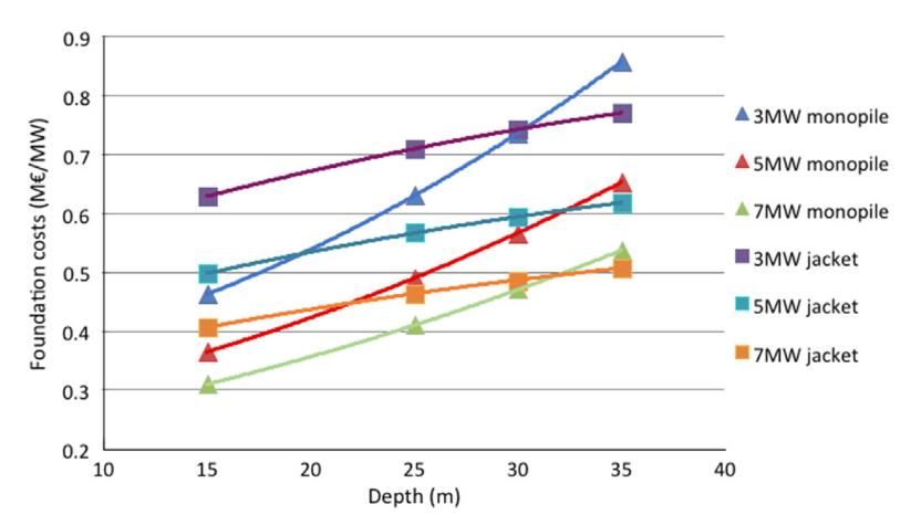
Figure 24: Impact of the size of the OWF in the CAPEX .............................................................. 38
Figure 25: CAPEX development with cumulative capacity installed. .......................................... 39
Figure 26: WACC historical development by literature and research......................................... 40
Figure 27: LCoE historic development ........................................................................................ 41
Figure 28: LCoE values against the cumulative capacity installed. ............................................. 42
Figure 29: LCoE development per country.................................................................................. 43
Figure 30: Wind technology patents development (IRENA). ...................................................... 45
Figure 31: Power Capacity analysis for the CAPEX. ..................................................................... 46
Figure 32: Energy analysis for the LCoE. ..................................................................................... 47
Figure 33: Historical and projected total installed capacity of offshore wind, 2000-2050. ........ 48
Figure 34: Credit Suisse estimations for the LCoE, by year of project commissioning. .............. 49

 List of tables:

Table 1: Included characteristics of the selected wind farms for the database elaborated. ..... 26
Table 2: OPEX approximation example ....................................................................................... 30
Table 3: Example table for the currency conversion and inflation correction. .......................... 31
Table 4: First and last year parameters comparison per country. .............................................. 43
Table 5: Filtered analysis learning equations. ............................................................................. 49
Table 6: Filtered analysis results for 2030 expected installed and generated power. ............... 49

 P a g e 7 | 65

Introduction

 In the eighteenth century, with the beginning of the industrial revolution, the
anthropogenic greenhouse gas emissions to the atmosphere have grown exponentially due to
industrial processes, causing what we now know as climate change. This change in atmospheric
conditions will result in a more unstable climate with the rise of extreme phenomena such as
droughts, hurricanes, storms, polar ice melting and a higher global average temperature.

 With the growing awareness of this many agreements have been created to reduce, or
at least control, the amount of emissions released into the atmosphere. The latest international
agreement has as long-term goal to keep the rise in global average temperature below 2 °C and
to limit the increase to 1.5 °C, since this would substantially reduce the risks and effects of
climate change. This is the Agreement of Paris.

 Many states signed the Paris Agreement in 2016 to combat climate change by
addressing greenhouse emissions through adaptation of the power systems, creating new
policies and founding sustainable projects, starting in 2020. By 2018, the agreement was signed
by 195 states and 184 are parties to it.

 The implementation of new forms of renewable energy generation are needed to satisfy
the increasing demand of energy while reducing the amount of greenhouse gases (GHG) emitted
to the atmosphere. The energy sector accounts for around 29% of total emissions, so renewable
energy technologies are rapidly developing in order to reduce them on time. Some of the
adopted strategies to support renewables are feed-in tariffs, quotas with tradable green energy
certificates, and competitive auctions initiated by the government making renewable energy
sources of major interest to investors (Del Río & Linares, 2014). Most of the renewable energy
technologies are relatively new, with commercial applications running for less than 20 years.
One of these new technologies is offshore wind, which was identified in 2013 as one of the key
technologies for achieving the 2020 targets (DECC & POST, 2013).

 Offshore wind energy (OWE) is a relatively new technology that has grown exponentially
since the beginning of 1991, with the first such wind farm in Vindeby, Denmark, having 11
turbines with a power of 450 kW, giving a total capacity of 4,95 MW.(Henderson, 2015). In 2018
Europe connected 409 new offshore wind turbines to the grid across 18 projects. This brought
2,649 MW of net additional capacity. Europe now has a total installed offshore wind capacity of
18,499 MW (Figure 1) (Windeurope, 2019).

 P a g e 8 | 65

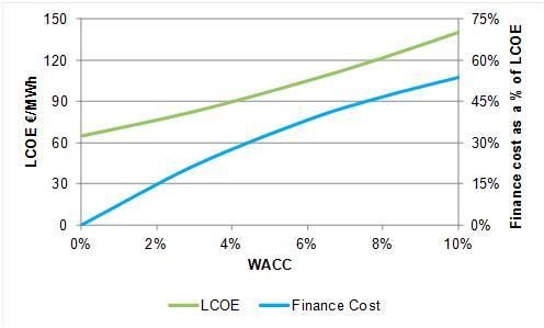
Figure 1: Offshore wind energy power installed in Europe in the period 2008-2018 (Windeurope, 2019).

 However, even if the energy cost for offshore wind energy (OWE) has been historically
higher than the average of conventional technologies, fossil or renewable, the evolution of OWE
in the last years shows a trend where this cost is decreasing (Figure 2¡Error! No se encuentra el
origen de la referencia.). This gives us the fact that OWE is expanding and, due to its advantages,
the trend may continue in the coming years. Some of the benefits are these by (NESGlobalTalent,
2016):

 • Turbines can be built sizeable, allowing for more energy collection from larger windmills,
 increasing the efficiency and the Power output.

 • The fact that the wind turbines are far out at sea makes them much less intrusive on the
 countryside, allowing for larger farms to be created per square mile.

 • There are typically higher wind speeds at sea and higher availability, as offshore
 conditions use to be windy. Also, there are no physical restrictions such as hills or
 buildings that could block the wind flow. These characteristics allows more energy to be
 generated at a time and with fewer interruptions than conventional onshore, due to the
 availability of wind.

 P a g e 9 | 65

Figure 2:Global Levelized Cost of Electricity from utility-scale renewable power generation technologies 2010-2017
(IRENA, 2018).

 However, some issues remain, such as that these cost-reduction effects have coincided
over the past few years and have alternated with cost increases, (Van der Zwaan, Rivera-Tinoco,
Lensink, & van den Oosterkamp, 2012) leading into a price development in the last years that,
gives not only decreasing market price for OWE, but also cost increment. This rise have been
studied by various researchers arguing that this could be caused by multiple factors, like the
changing price in commodities (Van der Zwaan et al., 2012), the increasing depth and distance
from shore for the projects (Voormolen, Junginger, & van Sark, 2016), the research investments
(Grafström & Lindman, 2017) beside others.

 Latest years cost developments for offshore wind farms (OWF) give an insight into the
sector's evolution. In 2013 in Germany the Levelized cost of electricity (LCoE) ranged between
114-190 €/MWh and it is expected to reach the 90 €/MWh in 2030 (Windeurope, 2019) while
in December 2017, the Netherlands approved a bid for its cheapest offshore project yet with €54.50
per megawatt-hour, for a site about 24 km off the coast. Just five months before, the winning bid for
the same site was €72.70 (McKinsey & Co). This means that the LCOE for new OWF is still
decreasing and it is expected to keep this way as shown in Figure 3¡Error! No se encuentra el
origen de la referencia. (Henderson, 2015). This will allow OWE to be competitive against
conventional fossil fuel energy.

 P a g e 10 | 65

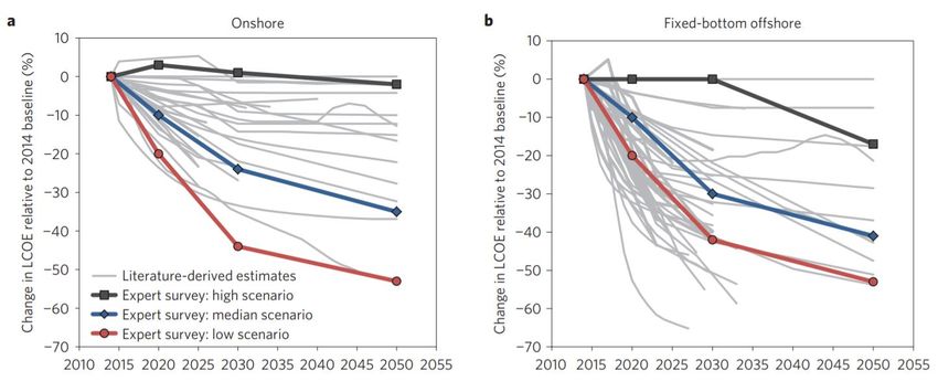
Figure 3:Evolution of the LCoE according to the cumulated installed capacity (Henderson, 2015)

 This cost reduction has been evolving with the growth of OWE in the recent years.
However, this trend has not being like this always. Once OWE was starting its commercialization
the cost started growing for the first years with a growing installed capacity. Some studies were
done to unravel how cost trends would be for the first years, in terms of LCoE and initial
investment, but with no success (M. Junginger, Faaij, & Turkenburg, 2005). The problems with
OWE cost are that it has changed in a different way than researchers expected, so the analysis
of past cost trends for the future presents irregular historical trends. However, as stated earlier,
trends in cost reduction are stabilizing, allowing some tools to be used to analyse future trends.
Experience curves are one of these tools.

 Experience curves are used to measure technological change by empirically quantifying
the impact of increased learning on the cost of production, and where learning is measured
through cumulative production or capacity (Lindman & Söderholm, 2012).

 Experience curves have been widely used in the energy market for multiple
technologies, including onshore wind energy, and can be used to analyse OWE's historical costs
and develop an analysis with future costs. However, when it comes to cost, performance and
technology used, offshore wind is different from onshore.

 While it has been proven that one-factor learning curve works with onshore wind
energy, in the past it has been shown that it does not work with offshore (Voormolen et al.,
2016). This could be caused by the fact that in onshore the turbine, even if this one also depends
on other factors, is around the 71% of the total cost of the project while in offshore this
represents around the 40% (Wüstemeyer, Madlener, & Bunn, 2015). This means that offshore
do not depended mainly on the upscaling of turbine production, but also on the technology
development, research, installation experience, project location and financial factors.

 So, besides the similarities between off-shore and on-shore wind energy technologies,
these have insurmountable differences that makes OWE different from on-shore, so the
experiences curves made for these will be different and adapted to the special mentioned
conditions for offshore. Factors like the newest installed power, R&D and the addition of new
data from OWF recently commissioned, and planned to be commissioned in the near future,
may give a good insight of the future LCoE (Voormolen et al., 2016).

 P a g e 11 | 65

Also, some expert’s elicitation surveys have been done before to predict the future
development of wind costs. This method is widely use and offers a close estimation of the future
expectations as shown in (Wiser et al., 2016a). With the experience curve method, it is possible
to build models for the future and make a differentiation between the possible values and
factors used. However, an expert elicitation would add reliability to the experience curves as in
Figure 4¡Error! No se encuentra el origen de la referencia..

Figure 4: Estimated change in LCOE comparing expert survey results with other forecasts (Wiser et al., 2016a)

 In Figure 4 the baseline of 2014 and the middle point in 2030 were built by asking to the
experts the expected average cost for the LCoE and by requesting details on five core input
components of LCoE: total upfront capital costs to build the project (CAPEX, €/kW); levelized
total annual operating expenditures over the project design life (OPEX, €kW/year); average
annual energy output (capacity factor, %); project design life considered by investors (years);
and costs of financing, in terms of the after-tax, nominal weighted-average cost of capital
(WACC, %) (Wiser et al., 2016a).

 As a result, numerous studies have been created to forecast the future trend for OWE,
but as it has not been until recently that the costs have begun to decline, previous studies have
not been able to evaluate future costs with this trend as an input. In this study the main
objectives are to unravel the costs historic trend from 2001 till the beginning of 2019 with the
data available nowadays, analyse it and elaborate some future expectation on how the costs will
develop considering the obtained learning rates for the LCoE and the CAPEX.

 Currently the majority of the offshore wind farms are installed in Europe. The UK has
the largest amount of installed offshore wind capacity in Europe, representing 43% of all
installations followed by Germany with 34%. Denmark remains the third largest market with 8%,
despite no additional capacity in 2017. The Netherlands (7%) and Belgium (6%) remain at the
third and fourth largest share respectively in Europe (Windeurope, 2019). Combined, the top
five countries englobe 98% of all grid-connected turbines in Europe. Therefore, these countries
will be the focus of the study to see the development of OWE.

 P a g e 12 | 65

Research questions

How has the LCoE developed historically and how will it develop in a medium-term (2030)
for off-shore wind energy projects in Europe?

 • Which factors affect the cost of OWE projects?
 • How variables, like CAPEX, CF, OPEX etc. have evolved?
 • How will the costs develop in the near future?

 P a g e 13 | 65

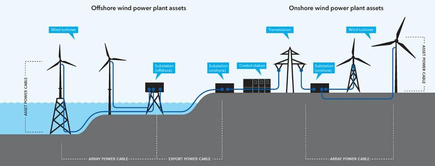
Theoretical background

In this section the theoretical background that forms the basis of this research is provided
describing the processes developed, the main theory needed and the factors calculations.

Offshore Wind Energy

 Offshore wind power or offshore wind energy (OWE) is the use of wind
farms constructed usually in the ocean on the continental shelf, to harvest wind energy to
generate electricity. Higher wind speeds are available offshore compared to on land, so offshore
wind power’s electricity generation efficiency is higher than onshore.

 An offshore wind farm has the typical layout of Figure 5 comparing it with onshore wind
farms. In offshore the turbine, that generates the electricity through the wind on the sea, needs
an extra part to fix it to the seabed, this is the foundation. The foundation represents an
important part of OWE and exist different kinds of them like monopile, the most used, jacked,
tripod etc. depending on the depth where the farm is installed and the seabed conditions.

 The farm is inter-connected with array power cables that takes the power to an offshore
substation that converts the electricity into a high tension current to minimize the losses in the
export cable. This export cable, as its name says, exports the electricity from offshore to
onshore, where this is converted again and connected to the conventional transmission system
for the grid.

Figure 5:Typical layout of an offshore and onshore wind farm (“DNV GL Blog,” n.d.).

 This OWFs have a cost that vary along time and from farm to farm. We can compose the
factors that affect the cost in four big groups that are:

 • Capital expenditures (CAPEX)
 • Operational expenditures (OPEX)
 • Annual energy production (AEP)
 • Financial Expenditures (FinEx, where the main factor is the WACC)

 P a g e 14 | 65

CAPEX

 The Capital expenditures (CAPEX) are the funds invested in the projects that include the
acquisition of all the components, the development phase, and the installation of the wind farm
until it has been fully commissioned. It does not include the financial expenditures and it is used
to check the initial investment done in a project and the cost per MW installed.

 The value chain that affect the CAPEX for an OWF could be classifies in the different
parts and processes involved in the fully commissioning of it, from the installation works, vessels
rental and engineering work and surveys to the manufactured goods needed in the farm (cables,
turbines, transformer etc.).

 These drivers that influence the final CAPEX may be categorised as either (i) ‘intrinsic’
or (ii) ‘external’, reflecting the extent to which offshore wind developers and energy
policymakers are able to influence them (Greenacre, Gross, & Heptonstall, 2010).

Intrinsic drivers include:

 • Depth, since the foundation type used, and the size, change with it and therefore the
 cost.

 •Distance, since the cables length is directly proportional to the distance from shore and
 the installing, operation and maintenance also increase with it.

 • Lack of competition in production of key components. Some products that influence
 greatly the cost are only produce by a few companies, like the turbines and the cabling
 (Windeurope, 2019). This lack of competition may lead into higher prices since there is
 no need into improving them like in a competitive market.

 • Supply chain/infrastructure bottlenecks. Some components do not have a specific
 market for themselves and they had to be “taken” from others. The best example are
 the installing vessels because, till recently, these were not specific for this task and were
 “taken” from oil and gas industry. This means that when the demand of oil and gas was
 high the vessels price increased.

 • Planning and consent.

External drivers of cost escalation include:

 • Cost of finance .

 • Exchange rates because some components must be purchased in different currencies.

 • Commodity prices, since a big fluctuation in these may influence the components
 manufacturing cost to some degree.

 P a g e 15 | 65

OPEX

 The Operational Expenditures (OPEX) in its definitions is “an ongoing cost for running a
product, business, or system”. It is usually confused with the Operation and Maintenance (O&M)
but these terms are not the same. Indeed, the O&M is part of the OPEX, representing the last
one also any other annual operating expenses. It is estimated that O&M is about 50% of the
total OPEX for offshore wind (IRENA, 2012). Other possible expenditures are the replacement of
parts, subsidies, depreciation and annual taxes (Gonzalez-Rodriguez, 2017).

 The Operating expenses include:

 ▪ License fees inherent of the energy generation offshore.
 ▪ Maintenance and repairs since the wind turbines require of continuous
 supervision and regular operations to guarantee their correct functioning.
 ▪ Supplies to replace broken parts, if necessary, and to replace those with normal
 wastage.
 ▪ Utilities for the crew that must remain offshore to work on the wind farm.
 ▪ Insurance coverage that helps mitigate risks during transportation, construction
 or operation of the asset.
 ▪ Salary and wages of the employees.
 ▪ Others.

AEP

 The Annual Energy Production (AEP) of a wind turbine is the total amount of electrical
energy that is produced over a year measured , in our case, in megawatt hours or terawatt
hours (MWh or TWh) (“Annual Energy Production. Windspire,” n.d.).

 The AEP depends on other important concept that is the Capacity Factor (CF). The
capacity factor is the average power generated on annual basis, divided by the rated peak
power. Let’s take a five-megawatt wind turbine. If it produces power at an annual average of
two megawatts, then its capacity factor is 40% (2÷5 = 0.40, i.e. 40%) (“Energy Numbers” n.d.).

These values have to be addressed for a few years to do an average since, if only one year is
taken, this value may be over, or below, estimated by one year with unusual atmospheric
conditions.

WACC
 OWF requires big investments, and the acquisition of these by the developers comes
with some financial expenditures that are summed to the final cost. To quantify these
expenditures the Weighted Average Cost of Capital (WACC) is the most common factor for this
kind of studies and found in plenty literature. A project’s WACC represents its blended cost of

 P a g e 16 | 65

capital across all sources, including common shares, preferred shares, and debt. The cost of
each type of capital is weighted by its percentage of total capital and they are added together
(Corporate Finance Institute, 2019).

Figure 6: WACC composition by (Corporate Finance Institute, 2019).

 Simplistically, WACC is the weighted average cost of finance, where the weighting is
based on the share of funds provided from different sources. For example, an equity provider
supplying half of the investment for a project expecting to release 15% and a lender provides
the other half as debt with a 5% interest rate, leading to a calculated ‘WACC’ of 10%. This
calculation works fine when you get your capital back at the end of the period (BVG Associates,
2016). But in offshore wind the value of the asset reduces to effectively zero over its life. So, the
finance payments must cover the repayment of the capital as well as the interest. This means
the true WACC is higher than previous calculation. Lenders providing funds for less than the
wind farm’s lifetime complicates the situation and increases the final true WACC.

 In the case of offshore wind projects it is required a large amount of capital with budgets
sometimes over 2 billion euros giving a typically debt-equity ratio around 70:30. The cost of debt
and equity is the result of several factors: general economic welfare, technology related risks
and in the case of offshore wind also policy risks (3E, 2013). This affects the WACC following
Equation 1 and in different way for each country since this is specifically calculated for each one.

Equation 1: WACC calculation

 % = ℎ ∗ (%) + ℎ ∗ (%)

 However, due to unstable and/or unpredictable policy frameworks with a change in risk
perception the WACC can change largely from year to year, which will have a significant effect
on the LCoE (Voormolen et al., 2016). To quantify the importance of WACC we can check Figure
7 where we can see that the change in the WACC for a project may change the LCoE largely. For

 P a g e 17 | 65

example a rise of 1% in the WACC would cause an increment in the cost pf energy of 5€/MWh
(Poudineh, Brown, & Foley, 2017).

 Figure 7: WACC fluctuations by (Poudineh et al., 2017).

Levelized cost of Electricity

 Levelized cost of electricity (LCoE) is often cited as a convenient summary measure of
the overall competitiveness of different generating technologies. It represents the per-MWh
cost (in discounted capital) of building and operating a generating plant over an assumed
financial life and duty cycle. Key inputs to calculating LCOE include capital costs, fuel costs, fixed
and variable operations and maintenance (O&M) costs, financing costs, and an assumed
utilization rate for each plant type (EIA, 2018).

 Following the formula used by Junginger (Voormolen et al., 2016) we got:

Equation 2: Levelized cost of electricity.

 + ∑ =1
 (1 + ) 
 =
 
 ∑ =1
 (1 + ) 
Where:

 i = the discount factor, similar to the Weighed Average Cost of Capital (WACC).

 t = the year of operation.
 P a g e 18 | 65

L = lifetime of the OWF.

 AEP = Annual energy production, based on the Capacity Factor (CP).

 OPEX = Operational expenditures.

 CAPEX = Capital expenditures.

 Other calculations for the LCoE have been launched to provide new nuances to the total
lifetime cost introducing development expenditures (DEVEX) and abandonment expenditures
(ABEX) (Megavind, 2015). The model developed by MEGAVIND has been proved to be an
accurate tool to calculate the LCoE for OWE but it also needs more specific data, sometimes
unavailable for the general public, to develop this LCoE (“ Megavind,” n.d.).

Experience and learning curves

 Experience curves have been largely used to develop economic models to see how the
production cost on a certain technology may change during time depending on one or various
factors. This approximation was previously used for onshore wind but very little for offshore
wind (Martin Junginger et al., 2004) and most of them failed to predict the trend for offshore
costs as there was no cost decrease until recently.

 One thing to mention is that it is common to use interchangeably the terms experience
curve and learning curve. They have different meanings, though. The Experience Curve is an
analytical tool designed to quantify the rate at which accumulated output experience, to date,
has an impact on total unit cost of a technology’s functional output. The learning curve is an
analytical tool designed to quantify the rate at which a cumulative work-hour or cost experience
allows an organization to reduce the amount of resources it needs to spend on performing a
task. The experience curve is broader than the curve of learning in terms of the costs covered,
the range of output during which cost reductions occur, and the causes of reduction
(“Experience and Learning Curve” n.d.).

 It is possible to talk about learning effects when a cumulative past output is negatively
related to the cost of creating the following unit. Looking at it from a mathematical way learning
curves can be described as:
Equation 3: Presence of learning efects.

 ∆ / 
 =

Here, C is the cost associated with the initial investment of an OWF (CAPEX) and Q is the
cumulative capacity of all the previous OWF (Dismukes & Upton, 2015).

 The one factor learning curves (OFLC) describe the cost of a given technology by the fact
that upscaling the production of this leads to a reduction in the cost, which is represented by
cumulative capacity or production of a certain technology (Kahouli-Brahmi, 2008). The usual way
to express the OFLC is by:
Equation 4: One factor learning curve equation (Yu, Van Sark, & Alsema, 2011).

 = − 
Where:

 C = Cost per unit of production.

 Ci = Cost of the first unit installed or produced.

 Q = cumulative capacity output.

 b = Learning index or experience index

 This OFLC depends on the economies of scale, where the cost of a certain good is
reduced in conjunction with the increase in production. Economies of scale exist when the
percent increase in output is greater than the percent increase in costs needed to achieve the
increase in output (Dismukes & Upton, 2015) . Or mathematically:
Equation 5: Economies of scale.

 ∆ / 
 = < 1
 ∆ / 
Where:

 ECQ = the “cost-cumulative output elasticity”.

 C = Cost associated with the initial investment to build the windfarm (CAPEX).

 q = Quantity produced.

 In this case, q is the installed capacity of an OWF in MW. If ECQ is equal to 1 then doubling
of C, will lead to doubling of q. If economies of scale are present, though, then the cost-output
elasticity will be less than one, and therefore doubling the cost will more than double the output
(Dismukes & Upton, 2015).

 However, the one factor learning curve only relates the cost change with the cumulative
capacity, ignoring other possible factors and effects like the ones of cumulative R&D
expenditures (Yu et al., 2011).

 Other option that incorporate the learning factor, or knowledge stock (KS) have been
introduce into the OFCL as a new variable (Klaassen, Miketa, Larsen, & Sundqvist, 2005):
Equation 6: Two factors learning curve equation.

 = − − 

 P a g e 20 | 65

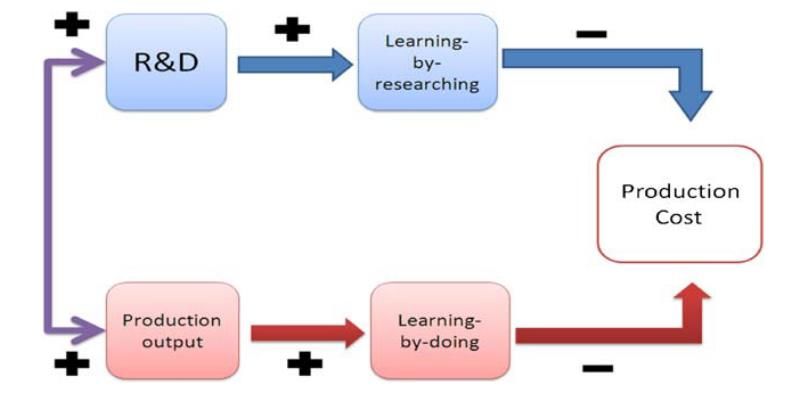
Where KS is equal to (1 − ή)KSt − 1 + RDt , where ή is the annual depreciation rate
and RDt the R&D expenditures at time t and α is the elasticity of learning by researching. This is
known as the Two factors learning curve (TFLC) (Yu et al., 2011).

 Figure 8: Relationships and feedbacks between R&D, production growth and production cost (Yu et al., 2011)

 The main issue is that the learning curve is for one product, while OWE farms consist of a
combination of several specific products such as turbines, tower, foundations, cabling, etc.
Experience curves therefore fits better, as the learning curve is really about a descent in labour
costs in a company, whereas the experience curve is to describe the total costs of a technology
in a whole industry while being based on the same concepts as learning curves. Second is that
this method only accounts the production but neglects other possible characteristics, like depth
and the distance to the shore in our case, that also influence the cost. Although, it can still be
expected that the cost go down by the development of several factors like the following ones
(Voormolen et al., 2016):

 • Learning-by-doing.
 • Learning-by-using.
 • Learning-by-search.
 • Standardization of the product.
 • Redesigning and upsizing of the product.

 These factors may reduce the cost of the products during a certain period. However, these
are not the only factors to consider. Other factors may cause also a cost change that in some
cases may even overcome the reduction gained by the experience like, the financial risk, political
framework, Capacity factor, etc.

 Because of the difficulty to obtain cost data for each factor the energy price is the main data
used and then this related to the cost for this new technology as described by Boston Consulting
Group (1968). However, with offshore energy this may be an issue since this new technology is
also associated with risks and uncertainties so, to be save, the profit margins are a bit higher
than the usual and may not represent perfectly the cost of production (Wüstemeyer et al.,
2015).
 P a g e 21 | 65

Definitions and scope

Current situation

 The first of this kind of installations can hardly being called offshore since the distance
from shore and depth are less and almost no comparable to the new farms. These first wind
farms were installed close to shore (>10km) and with water depth ranging 5-10m.

 Figure 9: Vindeby offshore wind farm

 While the main difference between the current situation and the past is that when
offshore technology began its commercial phase, it seemed to be a reasonable idea to use the
same technology for offshore wind farm as the one used in onshore with slight adjustments.
However, the needs for further offshore R&D and expertise was underestimated. Keeping in
mind that competition for onshore products is much stronger, and that marginal improvements
per fixed R&D expenditures are small, insufficient onshore investment can lead to distinct losses
in onshore market share (Wüstemeyer et al., 2015).

 One example of this problem is the 160MW wind farm Horns Rev in Denmark with 80
Vestas V80 turbines that were adapted for offshore usage (Richardson, 2010). Two years after
the commissioning, all wind turbines had to be removed for refurbishment, maintenance and
replacement works due to eminent transformer and generator problems (Sweet, 2008).
Companies tried to adapt onshore technology saving additional R&D investment. These soon
realised that OWF needed a new division and that it is not just an onshore extension. However,
optimizing products for offshore usage means at the same time making them inefficient for
onshore wind power, since additional features, such as an extended corrosion resistance, are
unnecessary cost drivers (Wüstemeyer et al., 2015).

 Since the firsts OWF the followed trend has been increasing the size and rated power of
the turbines, the depth and the distance from shore. This leaded in the period 2000-2015 in an
increase of the Capital Expenditures (CAPEX) from 1.5 M€/MW in 2000 to 4.0 M€/MW in 2010
and a decrease in the recent years 2015-2018 that is explained further in this paper.

 P a g e 22 | 65

Size and rated power

 The first turbines installed had a diameter around 65m and a capacity of 2MW while in
2018 the average rated capacity of new installed turbines was 6.8 MW (Figure 10¡Error! No se
encuentra el origen de la referencia.), 15% larger than in 2017 and rotors size of 160m. Since
2014 the average rated capacity of newly installed wind turbines has grown at an annual rate of
16% (Windeurope, 2019).

 Figure 10: Yearly average of newly installed offshore wind turbine rated capacity (MW)

 This trend in the size rise looks like will keep on track next years since it is already
confirmed the commercialization of a 10 MW and 164m rotor turbine by Vestas in the beginning
of 2021 and a 12 MW turbine by Haliade-X is under development for 2022 (International Energy
Agency, 2018).

 Figure 11: Evolution of the largest commercially available wind turbines

 P a g e 23 | 65

The main reason to explain this size trend is that the new turbines develop a higher
capacity factor to maximize CF and by hence the annual energy production (AEP) (Figure 12)
¡Error! No se encuentra el origen de la referencia.¡Error! No se encuentra el origen de la
referencia.. But the question is then, what is the CF we have been talking and, why the efforts
to increase it?

 So, the ratio between a turbine capacity and rotor area is the power density (W/m2). A
bigger rotor diameter leads to a lower power density so less energy (lower wind speeds) is
required to reach the rated capacity of a turbine. This leads into a higher CF as seen in Figure 12.

 Figure 12: Average offshore wind farm turbine size and capacity factors, 2010-2022 (IRENA)

 However, the turbine size has also positive effects in the Operation and Maintenance
(O&M) part since a powerful turbine requires less care and cost than multiple turbines with a
lower rated power (Ioannou, Angus, & Brennan, 2018). Due to this size changes each new wind
farm used different foundations, with a different pile diameter. If at a certain point an ideal
turbine size is reached, standardization may bring some advantages (Martin Junginger et al.,
2004). However, while there seems to be some room for cost reductions, this is unlikely to occur
since each OWF has different properties depending on the location like the average wind speed,
seabed conditions and distance from shore.

Depth and distance from shore

 Together with the size increase comes the depth and distance from shore. These two
depends on the project`s location and may influence the final cost of the project since the
distance increase the oil used by the vessels, the construction times, the cables length and the
O&M costs. The depth influence directly in the cost of the turbines foundations as shown in the
FLOW model by (Voormolen et al., 2016) in ¡Error! No se encuentra el origen de la referencia..
Although the foundations cost may represent, excluding transportation and installations,
around 19% of the CAPEX (Wüstemeyer et al., 2015) this could be more if the foundations
 P a g e 24 | 65

instead of being monopile is
 jacked, for example, or even
 more if these are floating since
 these are still under
 development.

 Since the depth is a
 factor that influence the overall
 CAPEX, it is a major concern to
 solve some of the issues
 involved. The actual trend goes
Figure 13: Cost of fountation depending on the depth by Voormolen. for OWF further from shore to
 search for new spots with high
quality winds. However, together with the distance comes a depth increase (Figure 14) till a
point where actual technologies like jacked and monopile structures wont suit the
requirements. New technologies, like floating foundations, are just starting to appear in the
market as commercial projects, like the 30 MW demonstration project that is currently in
operation in the UK since 2017. The Hywind Scotland Wind Farm has a nominal power capacity
of 30 MW, consists of five turbines of 6 MW each and uses a spar buoys design (Equinor, n.d.)
(International Renewable Energy Agency, 2018). After three months of operation, the Hywind
farm claimed to have achieved a remarkable average capacity factor of 65% (Equinor, 2018). The
advantages and expected development of this technology is developed futher in this research.

 Distance vs depth
 160
 140
 distance to shore (km)

 120
 100
 80
 60
 40
 20
 0
 0 5 10 15 20 25 30 35 40 45
 depth (m)

Figure 14: Depth change with the distance from shore

 P a g e 25 | 65

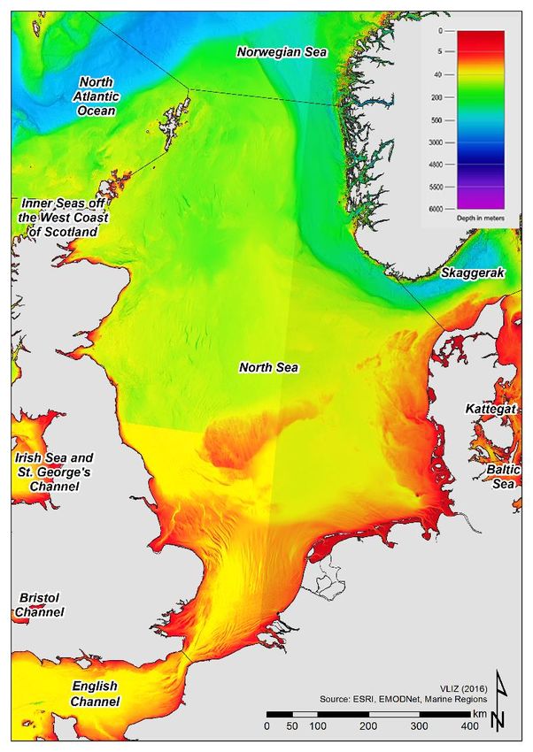
Methods

 In order to comprehend the cost trends and the future developments of offshore wind
energy the historic and current data from European OWFs has been analysed. The collected
data, in the majority of the cases, are: the commission date, the power of the OWF, the turbines
model, specifications and power, water depth, average distance of the farm from shore (in some
cases when the data was not available this was calculated by geographical approximation with
Google Earth), foundation type and OWF location. After that the parameters like the CAPEX and
the LCoE were calculated. In order to analyse the historic and actual price developments for
OWE all the possible and useful data has been collected and presented as in Table 1 with the
main OWFs in Germany, the Netherlands, Belgium, the UK and Denmark since these accumulate
97.6% of the total installed capacity in Europe (Windeurope, 2019). The original goal of the
analysis is to indicate how costs change during time due to these factors and analyse the effect
of scale and learning effects but also how any other financial and technical factors affect the
LCoE. In order to assess the reliability of the analysis, 86 existing OWFs have been included in
the database to calculate these trends from the selected European countries

 The data for the wind farms has been extracted mainly from (4C Offshore, n.d.) and
some gaps have been filled with literature review and online search. This database contains all
useful information about 86 European OWFs in Belgium, the UK, Germany, The Netherlands and
Denmark.
Table 1: Included characteristics of the selected wind farms for the database elaborated.

 Characteristics Unit/classification
 CAPEX M€/MW
 Commissioning date Month and year
 Capacity of the OWF MW
 Turbine capacity MW
 Turbine model Manufacturer and name
 Country BE, DE, DK, NL, UK
 Water depth m
 Foundation type Monopile, jacked, tripod, gravity based,
 floating.
 Distance to shore km
 Average capacity factor
 Status FC, UC, PG/UC, PC
 Rotor diameter m
 Expected lifetime years
 LCoE €/MWh
 WACC
 Cumulative installed capacity MW
 Cumulative generated energy TWh

 The water depth and distance from shore were specified for some projects while looking
for the information, but this was not possible for every windfarm. In those cases where the
information was not available it has been calculated through geographical approximation. This
means that for the distance from shore the location of the OWF, available for every farm in

 P a g e 26 | 65

4Coffshore, was taken and with Google earth measure the km from the coast. For the depth it
was necessary to use a map of the bottom of the North and Baltic sea like in Figure 15. However,
these were just approximations since the depth varies even inside the same OWF, so the exact
depth was very hard to get.

 Figure 15: North sea depth map (De Hauwere, 2012).

 The performance and Annual Energy Production of OWFs is based on the CF (capacity
factor). This has been obtained for OWFs in Germany, Denmark, the United Kingdom and
Belgium through (“Energy Numbers - Thinking about energy,” n.d.)(2018). However, the
Netherlands and some other windfarms from the mentioned countries were not available here
so the missing gaps were filled taking data from different websites like, OWE websites and
project developer´s websites where the expected annual production for the windfarms was
given so the CF could be easily calculated.

 The prices have been normalized into the same currency (€) and with the corrected
inflation, so all data is expressed in real 2019 Euros from its value in January. This has been done
by using the European inflation rates (Binder & Wieland, 2008). Also, it was necessary to convert
the different currencies into euros, so the historic conversion rates have been applied for British
pounds and Danish crowns (Fxtop, 2016).

 P a g e 27 | 65

Cumulative installed capacity and energy generation

 By adding the power of each OWF in order of commissioning date, the cumulative
installed capacity was calculated. This way, with the increasing availability of installed power, it
is possible to see the technology development.
Equation 7: Cumulative installed capacity.

 = ∑ ℎ 
 =1

 The cumulative energy generation follows a similar way than the cumulative installed
capacity. The average AEP for each windfarm is added following the order of commissioning
date. Although, it is important to consider that the OWF do not produce the same amount of
energy every always, since this may change largely depending on the meteorological conditions
of each year. However, the average numbers for the production are enough to have rough
amounts for the production.

Equation 8: Cumulative energy generation.

 = ∑ ∗ ℎ ∗ 8760ℎ
 =1

Calculating the LCoE

 The Levelized Cost of Electricity was calculated through the Equation 2 explained before.
However, there are some issues regarding this term that must be explained to understand the
results and the meaning of these.

 Our result for the LCoE is in €/MWh, this means that it will give the cost of the produced
energy considering the whole lifetime of the OWF or, in other words, it represents the per-MWh
cost of building and operating a generating plant over an assumed financial life and duty cycle.
The lifetime may change from one farm to another and this must be considered since the
information about the expected life of many farms was not available. Most of the farms have
values of 20 or 25 years, being 25 the most abundant. So, if the value was missing, 25 years have
been taken as default.

OPEX approximation

 The OPEX is certainly a factor subject to change from year to year and, as the CAPEX,
depends to a certain point on the distance from shore and the windfarm size. Figure 16 shows
the comparison of the breakdown of CAPEX and OPEX for a typical offshore wind farm (Crabtree,
Zappalá, & Hogg, 2015).

 P a g e 28 | 65

Figure 16: OPEX values in literature.

 Although the CAPEX and OPEX contribution to the final cost changes depending on the
reference source taken. Thus, wind farms are capital-intensive compared to conventional
sources of fossil fuel fired technologies such as a natural gas power plant, for which fuel charges
increase OPEX costs to typically between 40% and 70% of the LCOE.

 The real OPEX values for the studied windfarms are unavailable since companies are not
willing to share this because of the confidentiality of their accounts. However, some estimations
have been done in literature representing always values around the 27% of the total cost.

 Other way to estimate the OPEX is depending on the qualities of the OWFs through the
formula used in (Ioannou et al., 2018) when the characteristics of the farms matches the ones
used in this paper. These characteristics are:

 • Distance from shore between 15 and 65 km.
 • OWF capacity between 250 and 1000 MW.
 • Wind turbine rating between 2 and 7 MW.

 If the OWF specifications matches the required by this paper the Equation 9 is used to get
an approximation of the OPEX.

Equation 9 :OPEX approximation with 3 variables

 0.187
 = −6.349 ∗ 108 ∗ + 2.595 ∗ 10−19 ∗ exp(0.830 ∗ ) + 8.413 ∗ 105 ∗ + 9.506 ∗ 108

 There has been also reported a formula by IRENA to get an approximation of the OPEX
based in the Annual Energy Production (AEP) for an OWF.

 € 
 ( ) = 17 ∗
 1000000
 P a g e 29 | 65

It is appreciated that there are some ways to determine the OPEX and it was not possible
to decide which one is better so, in order to get the more realistic and accurate value, these
three methods have been used to calculate the OPEX. In the case that an OWF do not meet the
requirements to apply Ioannou’s formula only two estimations where made. Then the averages
from these were calculated and used as the OPEX value for further estimations. To explain better
the applied method, we have the next example:

Table 2: OPEX approximation example

 Method OPEX obtained

 Equation 6 53

 IRENA formula 45

 27% from CAPEX 47

 Final OPEX (45+47+53)/3 = 48.33

CAPEX calculation

 The CAPEX has been obtained through the initial investment cost. This means, that the
found total cost till the commissioning for each windfarm has been divided by the installed
power in MW, getting a result in million euros per Megawatt installed.

WACC approximation

 The WACC results from 2000 till 2014 have been extracted from the literature by
(Voormolen et al., 2016). For projects from 2015 the WACC it has been calculated using the
Equation 1 and getting online the values for the equity and debt. It has been possible also to get
some specific WACC for some projects, so this was taken when possible to get more accurate
results.

AEP calculation

 The annual energy production was available for some of the OWF in the developer’s
webpages. This production estimations works fine for those OWF that are too new to get reliable
enough information about the energy production.

 However, the best option was to get the real average production for the OWF but this
AEP was not available for every project and has been derived from the Capacity factor (Equation
10) that was found for certain projects (“Energy Numbers - Thinking about energy,” n.d.).
Equation 10: Annual energy production from the capacity factor

 = ∗ ∗ 8760ℎ/ 

 P a g e 30 | 65