MAX-AFFINE SPLINE INSIGHTS INTO DEEP GENERATIVE NETWORKS
←
→
Page content transcription
If your browser does not render page correctly, please read the page content below
Under review as a conference paper at ICLR 2021

M AX -A FFINE S PLINE I NSIGHTS INTO
D EEP G ENERATIVE N ETWORKS
 Anonymous authors
 Paper under double-blind review

                                            A BSTRACT
         We connect a large class of Deep Generative Networks (DGNs) with spline oper-
         ators in order to analyze their properties and limitations and suggest new opportu-
         nities. By characterizing the latent space partition and per-region affine mappings
         of a DGN, we relate the manifold dimension and approximation error to the sam-
         ple size, provide a theoretically motivated “elbow method” to infer the intrinsic
         dimensionality of the manifold being approximated, study the (not always) ben-
         eficial impact of dropout/dropconnect, and demonstrate how a DGN’s piecewise
         affine generated manifold can be “smoothed” to facilitate latent space optimiza-
         tion as in inverse problems. The per-region affine subspace defines a local coor-
         dinate basis; we provide necessary and sufficient conditions relating those basis
         vectors with disentanglement and demonstrate how to interpret the DGN’s learned
         parameters. We also derive the output probability density that is mapped onto the
         generated manifold in terms of the latent space density, which enables the com-
         putation of key statistics such as its Shannon entropy. This finding enables us to
         highlight the source of training instabilities when the target density is multimodal:
         as the modes move further apart and/or are more concentrated, the singular values
         of the approximant DGN per-region mappings increase, leading to overly large
         layer weights and causing training instabilities.

1   I NTRODUCTION
Deep Generative Networks (DGNs), which map a low-dimensional latent variable z to a higher-
dimensional generated sample x, have made enormous leaps in capabilities in recent years. Popular
DGNs include Generative Adversarial Networks (GANs) Goodfellow et al. (2014) and their variants
Dziugaite et al. (2015); Zhao et al. (2016); Durugkar et al. (2016); Arjovsky et al. (2017); Mao et al.
(2017); Yang et al. (2019); Variational Autoencoders Kingma & Welling (2013) and their variants
Fabius & van Amersfoort (2014); van den Oord et al. (2017); Higgins et al. (2017); Tomczak &
Welling (2017); Davidson et al. (2018); and flow-based models such as NICE Dinh et al. (2014),
Normalizing Flow Rezende & Mohamed (2015) and their variants Dinh et al. (2016); Grathwohl
et al. (2018); Kingma & Dhariwal (2018).
While DGNs are easy to describe and analyze locally in terms of simple affine operators and scalar
nonlinearities, a general framework for their global structure has remained elusive. In this paper,
we take a step in the direction of a better theoretical understanding of DGNs constructed using con-
tinuous, piecewise affine nonlinearities by leveraging recent progress on max-affine spline operators
(MASOs) Balestriero & Baraniuk (2018b). Our main contributions are as follows:
[C1] We characterize the piecewise-affine manifold structure of a DGN’s generated samples
(Sec. 3.1), including its intrinsic dimension, which sheds new light on the impact of techniques
like dropout (Sec. 3.2) and provides practitioners with sensible design principles for constructing a
desired manifold (Sec. 3.3).
[C2] We characterize the local coordinates of a DGN’s generated manifold and the inverse mapping
from the generated data points x back to the latent variables z. This sheds new insights on the DGN
architectures and suggests a novel discrete optimization problem for DGN inversion and inverse
problem applications (Sec. 4.1). Armed with this result, we derive necessary conditions on the
DGN per-region affine mappings for disentanglement, to interpret the disentangled mappings, and
to draw new links between DGNs and adaptive basis methods (Sec. 4.2). We also demonstrate
how to smooth a DGN’s generated continuous piecewise affine manifold in a principled way, which
enables new approaches for (smooth) manifold approximation (Sec. 4.3).

                                                  1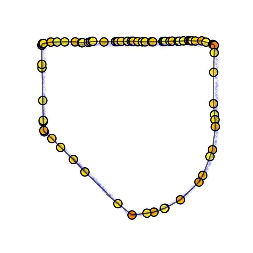
Under review as a conference paper at ICLR 2021

[C3] We provide an input-output formula for a DGN that enables us to derive the analytical prob-
ability density on the generated manifold that is induced by the latent space (Section 5.1). We use
this result to derive the analytical form of this density for several interesting settings and demon-
strate that there exists a crucial link between the DGN partition, the singular values of the per-region
affine mappings, and the Shannon entropy of the output density. This provides a new lens through
which to study the difficulty of generating multidimensional, low-entropy distributions using DGNs
(Section 5.2).
Reproducible code for the various experiments and figures will be provided on Github upon com-
pletion of the review process. Proofs of our results are provided in Appendix F.
2   BACKGROUND
Deep Generative Networks. A deep generative network (DGN) is an operator GΘ with parameters
Θ mapping a latent input z ∈ RS to an observation x ∈ RD by composing L intermediate layer
mappings g` , ` = 1, . . . , L. We precisely define a layer g ` as comprising a single nonlinear operator
composed with any (if any) preceding linear operators that lie between it and the preceding nonlinear
operator. Examples of linear operators are the fully connected operator (affine transformation with
weight matrix W ` and bias vector b` ), or the convolution operator (circulent W ` matrix); examples
of nonlinear operators are the activation operator (applying a scalar nonlinearity such as the ubiqui-
tous ReLU), or the pooling operator (dimensionality reduction given a maximum operator). Precise
definitions of these operators can be found in Goodfellow et al. (2016). We will omit Θ from the fΘ
operator for conciseness unless needed.
                                                                `−1                                     `
Each layer g ` transforms its input feature map v `−1 ∈ RD          into an output feature map v ` ∈ RD
with in particular v 0 := z, D0 = S, and vL := x, DL = D. In this paper, we focus on DGNs,
where in general S ≤ D and in some cases S  D. In such framework z is interpreted as a latent
representation, and x is the generated/observed data, e.g, a time-serie or image. The feature maps v `
can be viewed equivalently as signals, flattened column vectors, or tensors depending on the context.
Max-Affine Spline Deep Networks. A max-affine spline operator (MASO) concatenates indepen-
dent max-affine spline (MAS) functions, with each MAS formed from the point-wise maximum of R
affine mappings Magnani & Boyd (2009); Hannah & Dunson (2013). For our purpose each MASO
will express a DN layer and is thus an operator producing a D` dimensional vector from a D`−1
dimensional vector and is formally given by

                             MASO(v; {Ar , br }R
                                               r=1 ) = max Ar v + br ,                               (1)
                                                         r=1,...,R

                  `    `−1                               `
 where Ar ∈ RD ×D        are the slopes and br ∈ RD are the offset/bias parameters and the max-
imum is taken coordinate-wise. For example, a layer comprising a fully connected operator with
weights W ` and biases b` followed by a ReLU activation operator corresponds to a (single) MASO
with R = 2, A1 = W ` , A2 = 0, b1 = b` , b2 = 0. Note that a MASO is a continuous piecewise-
affine (CPA) operator Wang & Sun (2005).
The key background result for this paper is that the layers of DNs constructed from piecewise affine
operators (e.g., convolution, ReLU, and max-pooling) are MASOs Balestriero & Baraniuk (2018b;a):
                                                                                         `−1
           ∃R ∈ N∗ , ∃{Ar , br }R                          R
                                r=1 s.t. MASO(v; {Ar , br }r=1 ) = f` (v), ∀v ∈ R
                                                                                  D
                                                                                               ,     (2)

making the entire DGN a composition of MASOs.
The CPA spline interpretation enabled from a MASO formulation of DGNs provides a powerful
global geometric interpretation of the network mapping f based on a partition of its input space RS
into polyhedral regions and a per-region affine transformation producing the network output. The
partition regions are built up over the layers via a subdivision process and are closely related to
Voronoi and power diagrams Balestriero et al. (2019). We now propose to greatly extend such CPA
spline driven insights to carefully characterize and understand DGNs as well as providing theoretical
justifications to various observed behaviors such as mode collapse.

3   I MPORTANCE OF THE D EEP G ENERATIVE N ETWORK D IMENSION
In this section we study the properties of the mapping GΘ : RS → RD of a DGN comprising L
piecewise-affine MASO layers.

                                                   2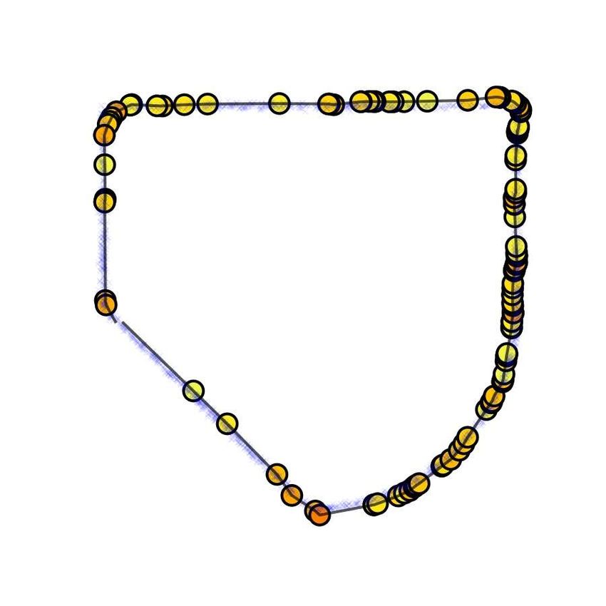
Under review as a conference paper at ICLR 2021

                                                            Figure 1: Visual depiction of Thm. 1 with a (random)
                                                            generator G : R2 7→ R3 . Left: generator input space
                                                            partition Ω made of polytopal regions. Right: gener-
                                                            ator image Im(G) which is a continuous piecewise
                                                            affine surface composed of the polytopes obtained
                                                            by affinely transforming the polytopes from the in-
                                                            put space partition (left) the colors are per-region and
                                                            correspond between left and right plots. This input-
                                                            space-partition / generator-image / per-region-affine-
                                                            mapping relation holds for any architecture employing
                                                            piecewise affine activation functions. Understanding
                                                            each of the three brings insights into the others, as we
                                                            demonstrate in this paper.

3.1 I NPUT-O UTPUT S PACE PARTITION AND P ER -R EGION M APPING
As was hint in the previous section, the MASO formulation of a DGN allows to express the (entire)
DGN mapping G (a composition of L MASOs) as a per-region affine mapping
                                         (Aω z + bω ) 1z∈ω ,
                                     X
                           G(z) =                             z ∈ RS ,                        (3)
                                         ω∈Ω
                                                                        0
with ∪ω∈Ω ω = R and ∀(ω, ω ) ∈ Ω2 , ω 6= ω 0 , ω ◦ ∩ ω ◦ = ∅, with (·)◦ the interior opera-
                      S              0

tor Munkres (2014), and Aω ∈ RD×S , bω ∈ RD the per-region affine parameters. The above
comes naturally from the composition of linear operators interleaved with continuous piecewise
affine which are current activation functions (ReLU Glorot et al. (2011), leaky-ReLU Maas et al.
(2013), absolute value Bruna & Mallat (2013), parametric ReLU He et al. (2015) and the likes)
and/or max-pooling. For a dedicated study of the partition Ω we refer the reader to Zhang et al.
(2018); Balestriero et al. (2019).
In order to study and characterize the DGN mapping (3), we make explicit the formation of the
per-region slope and bias parameters. The affine parameters Aω , bω can be obtained efficiently by
using an input z ∈ ω and the Jacobian (J) operator, leading to
                      L−1
                                                 !
                      Y
                                   L−i
                                           L−i
                                                    = diag σ̇ L (z) W L . . . diag σ̇ 1 (z) W 1 , (4)

 Aω = (Jz G)(z) =          diag σ̇     (ω) W
                          i=0
         `
where σ̇ (z) is the pointwise derivative of the activation function of layer ` based on its input
W ` z `−1 + b` , which we note as a function of z directly. The diag operator simply puts the given
vector into a diagonal square matrix. For convolutional layers (or else) one can simply replace the
corresponding W ` with the correct slope matrix parametrization as discussed in Sec. 2. Notice that
since the employed activation functions σ ` , ∀` ∈ {1, . . . , L} are piecewise affine, their derivative
is piecewise constant, in particular with values [σ̇ ` (z)]k ∈ {α, 1} with α = 0 for ReLU, α = −1
for absolute value, and in general with α > 0 for Leaky-ReLU for k ∈ {1, . . . , D` }. We denote
the collection of all the per-layer activation derivatives [σ̇ 1 (z), . . . , σ̇ L (z)] as the activation pattern
of the generator. Based on the above, if one already knows the associated activation pattern of a
region ω, then the matrix Aω can be formed directly by using them without having access to an
input z ∈ ω. In this case, we will slightly abuse notation and denote those known activation patterns
as σ̇ ` (ω) , σ̇ ` (z), z ∈ ω with ω being the considered region. In a similar way, the bias vector is
obtained as
                                     L−1
                                          " L−`−1                                    !                  #
                                     X         Y
                                 L                           L−i
                                                                         L−i                   `
                                                                                                     `
         bω = G(z) − Aω z = b +                      diag σ̇       (ω) W                diag σ̇ (ω) b .
                                         `=1      i=0
The bω vector can be obtained either from a sample z ∈ ω using the left part of the above equation
or based on the known region activation pattern using the right hand side of the equation.
Theorem 1. The image of a generator G employing MASO layers is made of connected polytopes
corresponding to the polytopes of the input space partition Ω, each being affinely transformed by
the per-region affine parameters as in
                                                        [
                        Im(G) , {G(z) : z ∈ RS } =          Aff(ω; Aω , bω )                  (5)
                                                                  ω∈Ω

                                                        3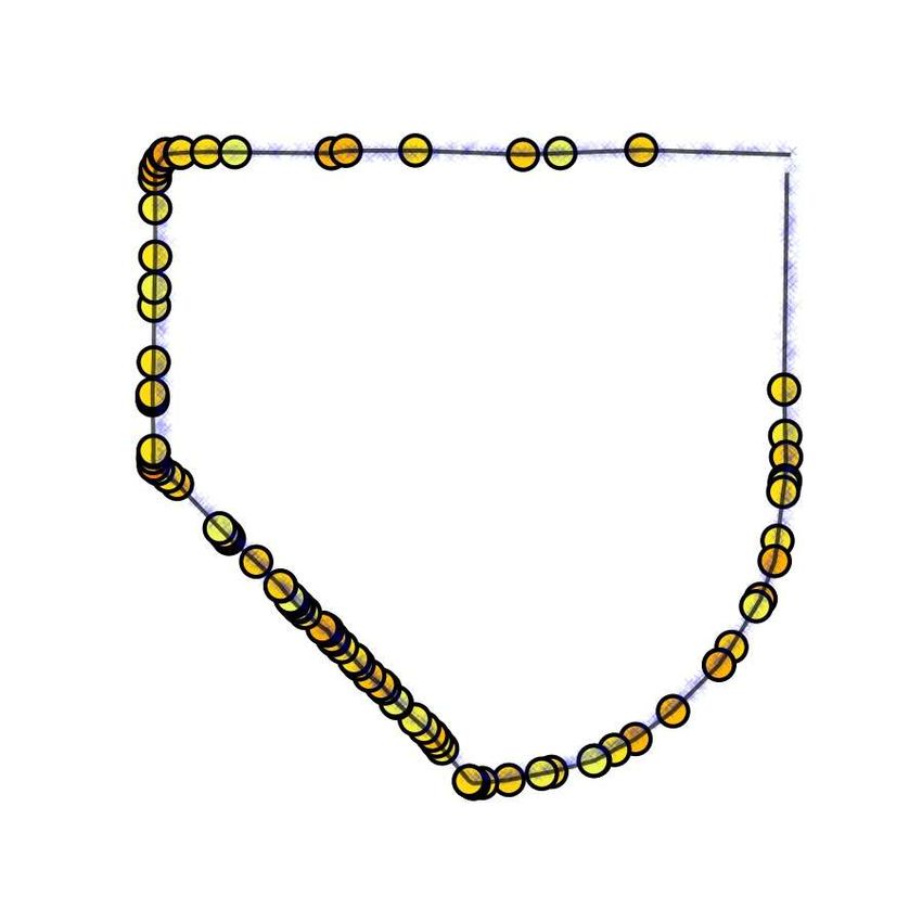
Under review as a conference paper at ICLR 2021

              Dropout 0.1            Dropout 0.3             Dropconnect 0.1          Dropconnect 0.3

dim(G (ω))

                                            layers’ width
Figure 2: Impact of dropout and dropconnect on the intrinsic dimension of the noise induced generators for
two “drop” probabilities 0.1 and 0.3 and for a generator G with S = 6, D = 10, L = 3 with varying
width D1 = D2 ranging from 6 to 48 (x-axis). The boxplot represents the distribution of the per-region
intrinsic dimensions over 2000 sampled regions and 2000 different noise realizations. Recall that the intrinsic
dimension is upper bounded by S = 6 in this case. Two key observations: first dropconnect tends to producing
DGN with intrisic dimension preserving the latent dimension (S = 6) even for narrow models (D1 , D2 ≈ S),
as opposed to dropout which tends to produce DGNs with much smaller intrinsic dimension than S. As a
result, if the DGN is much wider than S, both techniques can be used, while in narrow models, either none or
dropconnect should be preferred.

with Aff(ω; A, b) = {Az + b : z ∈ ω}; we will denote for conciseness G(ω) , Aff(ω; Aω , bω ).
The above result is pivotal in bridging the understanding of the input space partition Ω, the per-
region affine mappings Aω , bω , and the generator mapping. We visualize Thm. 1 in Fig. 1 to make
it clear that characterizing Aω alone already provides tremendous information about the generator,
as we demonstrate in the next section.
3.2 G ENERATED M ANIFOLD I NTRINSIC D IMENSION
We now turn into the intrinsic dimension of the per-region affine subspaces G(ω) that are the pieces
forming the generated manifold. In fact, as per (5), its dimension depends not only on the latent
dimension S but also on the per-layer parameters.
Proposition 1. The intrinsic dimension
                                      of the affine subspace G(ω)) (recall (5)) has the following

upper bound: dim(G(ω)) ≤ min S, min`=1,...,L rank diag(σ̇ ` (ω))W `           .
We make two observations. First, we see that the choice of the nonlinearity
(i.e., the choice of α) and/or the choice of the per-layer dimensions are the
key elements controlling the upper bound of dim(G). For example, in the
case of ReLU (α = 0) then dim(G(ω)) is directly impacted by the number
of 0s in σ̇ ` (ω) of each layer in addition of the rank of W ` ; this sensitivity
does not occur when using other nonlinearities (α 6= 0). Second, “bottle-             Figure 3: DGN with
neck layers” (layers with width D` smaller than other layers) impact di-              dropout trained (GAN)
rectly the dimension of the subspace and thus should be carefully employed            on a circle dataset (blue
based on the a priori knowledge of the target manifold intrinsic dimension.           dots); dropout turns a
In particular, if α 6= 0 and the weights are random (such as at initialization)       DGN into an ensemble
then one has almost surely dim(G(ω)) ≤ min(S, min`=1,...,L D` ).                      of DGNs (each dropout
                                                                                      realization is drawn in a
Application: Effect of Dropout/Dropconnect. Noise techniques, such as                 different color).
dropout Wager et al. (2013) and dropconnect Wan et al. (2013); Isola et al. (2017), alter the per-
region affine mapping in a very particular way impact the per-region affine mapping. Those tech-
niques perform an Hadamard product of iid Bernoulli random variables against the feature maps
(dropout) or against the layer weights (dropconnect); we denote a DGN equipped with such tech-
nique and given a noise realization by G where  includes the noise realization of all layers; note
that G now has its own input space partition Ω . We provide explicit formula of the piecewise
affine deep generative network in Appendix J. In a classification setting, those techniques have been
thoroughly studied and it was shown that adding dropout/dropconnect to a DN classifier turned
the network into an ensemble of classifiers Warde-Farley et al. (2013); Baldi & Sadowski (2013);
Bachman et al. (2014); Hara et al. (2016).
Proposition 2. Adding dropout/dropconnect to a deep generative network G produces a (finite)
ensemble of generators G , each with per-region intrinsic dimension 0 ≤ dim(G (ω )) ≤
maxω∈Ω dim(G(ω)) for ω ∈ Ω , those bounds are tight.
We visualize this result in Fig. 2, where we observe how different noise realizations produce slightly
different generators possibly with different per-region dimension. By leveraging the above and

                                                      4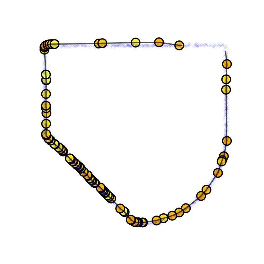
Under review as a conference paper at ICLR 2021

                                                                                 blue: N = 100, green: N = 1000

width of the MLP layers

                                                         Minimum error E ∗
                dropout probability                           DGN latent dimension S, (S ∗ in red)
Figure 4: Left: final training negative ELBO (smaller is better) for a MLP DGN (S = 100 in red) on MNIST
with varying width (y-axis) and dropout rates (x-axis) of the DGN (decoder); we observe that the impact of
dropout on performances depends on the layer widths (CIFAR10 results can be seen in Fig. 9). Right:Minimal
approximation error (E ∗ ) for a target linear manifold (S ∗ = 5, in red), with increasing dataset size from 100
to 1000 (blue to green) and different latent space dimensions S (x-axis), the E ∗ = 0 line is depicted in black.
This demonstrates (per Thm. 2) that whenever S̃ < S ∗ , the training error E ∗ increases with the dataset size N .

Thm. 1 we can highlight a potential limitation of those techniques for narrow models (D` ≈ S)
for which the noise induced generators will tend to be have a per-region intrinsic dimension smaller
than S hurting the modeling capacity of those generators. On the other hand, when used with wide
DGNs (D`  S), noise induced generators will maintain an intrinsic dimension closer to the one
of the original generator. We empirically demonstrate the impact of dropout into the dimension
of the DGN surface in Fig. 3; and reinforce the possibly detrimental impact of employing large
dropout rates in narrow DNs in Fig. 4. Those observations should open the door to novel technique
theoretically establishing the relation between dropout rate, layer widths, and dimensionality of the
desired (target) surface to produce.

From the above analysis we see that one should carefully consider the use of dropout/dropconnect
based on the type of generator architecture that is used and the desired generator intrinsic dimension.

3.3                       I NTRINSIC D IMENSION AND T HE E LBOW M ETHOD FOR D EEP G ENERATIVE N ETWORKS
We now emphasize how the DGN dimension S̃ , maxω dim(G(ω)) impacts the training error
loss and training sample recovery. We answer the following question: Can a generator generate N
training samples from a continuous S ∗ dimensional manifold if S̃ < S ∗ ? Denote the empirical error
                                                        ∗
                                                                    PN
measuring the ability to generate the data samples by EN  = minΘ n=1 minz kGΘ (z) − xn k, a
standard measure used for example in Bojanowski et al. (2017). We now demonstrate that if S̃ < S ∗
       ∗
then EN   increases with N for any data manifold.

Theorem 2. Given the intrinsic dimension of a target manifold S ∗ , then for any finite DGN with
smaller intrinsic dimension (S̃ < S ∗ ), there exists a N 0 ∈ N+ such that for any dataset size N2 >
N1 ≥ N 0 ≥ N of random samples from the target manifold one has EN      ∗
                                                                           = 0 and EN∗
                                                                                       2
                                                                                         > EN ∗
                                                                                                1
                                                                                                  .
From the above result, we see that, even when fitting a linear manifold, whenever there is a bottle-
neck layer (very narrow width) collapsing the DGN intrinsic dimension below the target manifold
dimension S ∗ , then as the dataset size exceeds a threshold, as the training error will increase. For
illustration, consider a dataset formed by a few samples from a S ∗ dimensional affine manifold. If
the number of samples is small, even a DGN with intrinsic dimension of 1 (thus producing a 1D
continuous piecewise affine curve in RD ) can fit the dataset. However, as the dataset size grows, as it
will become impossible for such a low dimension (even though nonlinear) manifold to go through all
the samples. We empirically observe this result in Fig. 4 (the experimental details are given in Ap-
pendix I). This should open the door to developing new techniques a la “Elbow method” Thorndike
(1953); Ketchen & Shook (1996) to estimate intrinsic dimensions of manifolds based on studying
the approximation error of DGNs.

The above results are key to understanding the challenges and importance of the design of DGN
starting with the width of the hidden layers and latent dimensions in conjunction with the choice of
nonlinearities and constraints on W ` of all layers.

                                                                             5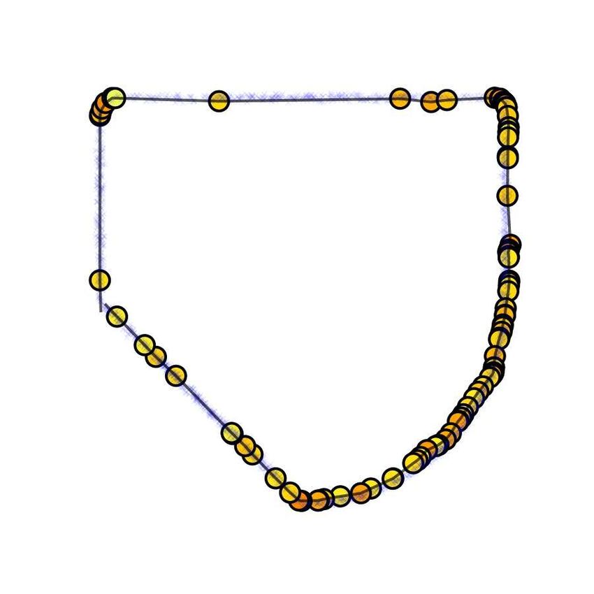
Under review as a conference paper at ICLR 2021

4   P ER -R EGION A FFINE M APPING I NTERPRETABILITY, M ANIFOLD
    S MOOTHING , AND I NVERSE P ROBLEMS
We now turn to the study of the local coordinates of the affine mappings comprising a DGN’s
generated manifold.
4.1 D EEP G ENERATIVE N ETWORK I NVERSION
We now consider the task of inverting the DGN mapping to retrieve z0 from x = G(z0 ). Note that
we use the term “inversion” only in this way, since, in general, Im(G) is a continuous piecewise
affine surface in RD , and thus not all x ∈ RD can be mapped to a latent vector that would generate
x exactly.
First, we obtain the following condition relating the per-region dimension to the bijectivity of the
mapping. Bijectivity is an important property that is often needed in generators to allow uniqueness
of the generated sample given a latent vector as well as ensuring that a generated sample has a
unique latent representation vector. That is, following the above example, we would prefer that only
a unique z0 produces x. Such uniqueness condition is crucial in inverse problem applications Lucas
et al. (2018); Puthawala et al. (2020).
Proposition 3. A DGN employing leaky-ReLU activation functions is bijective between its domain
RS and its image Im(G) iff dim(Aff(ω, Aω , bω )) = S, ∀ω ∈ Ω, or equivalently, iff rank(Aω ) =
S, ∀ω ∈ Ω.
Prior leveraging this result for latent space characterization, we derive an inverse of the genera-
tor G that maps any point from the generated manifold to the latent space. This inverse is well-
defined as long as the generator is injective, preventing that ∃z1 6= z2 s.t. G(z1 ) = G(z2 ).
Assuming injectivity, the inverse of G on a region G(ω) in the output space is obtained by
                     −1 T
G−1
  ω (x) = Aω Aω
                 T
                          Aω (x − bω ), ∀x ∈ G(ω) leading to G−1  ω (G(ω)) = ω, ∀ω ∈ Ω. Note that
                T
                     −1
the inverse Aω Aω        is well defined as Aω is full column rank since we only consider a generator
with S̃ = S. We can then simply combine the region-conditioned inverses   Pto obtain the overall gen-
erator inverse; which is also a CPA operator and is given by G−1 (x) = ω∈Ω G−1     ω (x)1{x∈G(ω)} .
In particular, we obtain the following result offer new perspective of latent space optimization and
inversion of DGNs.
Proposition 4. Given a sample x = G(z0 ), inverting x can be done via minz kx − G(z)k22
(standard technique, see ), but can also be done via minω∈Ω kx − G(G−1                  2
                                                                                ω (x))k2 , offering new
solutions from discrete combinatorial optimization to invert DGNs.
Recalling that there is a relation between the per-layer region activation r from Eq. 2 and the induced
input space partition, we can see how the search through ω ∈ Ω as given in the above result can
further be cast as an integer programming problem Schrijver (1998). For additional details on this
integer programming formulation of DN regions, see Tjeng et al. (2017); Balestriero et al. (2019)
and Appendix G.
We leveraged Aω as the basis of Aff(ω; Aω , bω ) in order to derive the inverse DGN mapping,
we now extend this analysis by linking Aω to local coordinates and adaptive basis to gain further
insights and interpretability.
4.2 P ER -R EGION M APPING AS L OCAL C OORDINATE S YSTEM AND D ISENTANGLEMENT
Recall from (5) that a DGN is a CPA operator. Inside region ω ∈ Ω, points are mapped to the
output space affine subspace which is itself governed by a coordinate system or basis (Aω ) which
we assume to be full rank for any ω ∈ Ω through this section.
The affine mapping is performed locally for each region ω, in a manner similar to an “adaptive
basis” Donoho et al. (1994). In this context, we aim to characterize the subspace basis in term of
disentanglement, i.e., the alignment of the basis vectors with respect to each other. While there is
no unique definition for disentanglement, a general consensus is that a disentangled basis should
provide a “compact” and interpretable latent representation z for the associated x = G(z). In
particular, it should ensure that a small perturbation of the dth dimension (d = 1, . . . , S) of z
implies a transformation independent from a small perturbation of d0 6= d Schmidhuber (1992);
Bengio et al. (2013). That is, hG(z) − G(z + δd ), G(z) − G(z + δd0 )i ≈ 0 with δd a one-
hot vector at position d and length S Kim & Mnih (2018). A disentangled representation is thus
considered to be most informative as each latent dimension imply a transformation that leaves the
others unchanged Bryant & Yarnold (1995).

                                                  6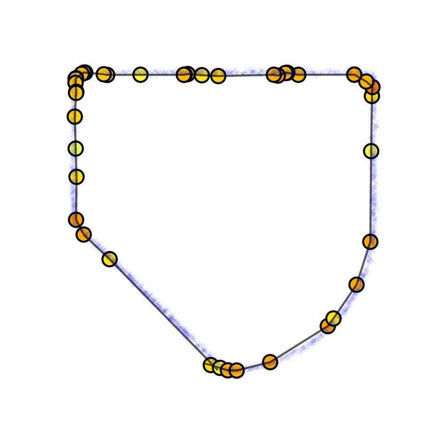
Under review as a conference paper at ICLR 2021

                    FC GAN   CONV GAN   FC VAE   CONV VAE   Figure 5: Visualization of a single basis vectors [Aω ].,k before and

initial
                                                            after learning obtained from a region ω containing the digits 7, 5, 9,
                                                            and 0 respectively, for GAN and VAE models made of fully con-
                                                            nected or convolutional layer (see Appendix E for details). We ob-
                                                            serve how those basis vectors encodes: right rotation, cedilla exten-
learned

                                                            sion, left rotation, and upward translation respectively allowing in-
                                                            terpretability into the learn DGN affine parameters.

                      β = 0.999             β = 0.9                β = 0.5
Generated surface

                                                                                               MNIST               CIFAR10

                                                                                      CNN
                                                                                                  β                    β

Figure 6: Left: Depiction of the DGN image Im(G) for different values of smoothing β; clearly the smooth-
ing preserves the overall form of the generated surface while smoothing the (originally) non-differentiable
parts. No other change is applied on G. Right: Negative ELBO (lower is better, avg. and std. over 10 runs) for
different DGNs (VAE trained) with CNN architecture with varying smoothing parameters β. Regardless of the
dataset, the trend seems to be that smoother/less-smooth models produce better performance in CNNs.

Proposition 5. A necessary condition for disentanglement is to have “near orthogonal” columns,
i.e., h[Aω ].,i , [Aω ].,j i ≈ 0, ∀i, 6= j, ∀ω ∈ Ω.
We provide in Table 1 in Appendix H the value of kQω − Ik2 with Qω ∈ [0, 1]S×S the matrix
of cosine angles between basis vector of Aω for 10,000 regions sampled randomly and where we
report the average over the regions and the maximum. Finally, this process is performed over 8
runs, the mean and standard deviation are reported in the table. We observe that there does not
seem to be a difference in the degree of disentanglement different GAN and VAE; however, the
topology, fully connected vs. convolution, plays an important part, favoring the former. Additionally,
Fig. 5 visualizes one of the basis vectors of four different DGNs trained on the MNIST dataset with
S = 10. Interpretability of the transformation encoded by the dimension of the basis vector can be
done as well as model comparison such as blurriness of VAE samples that is empirically observed
across datasets Zhao et al. (2017); Huang et al. (2018). To visually control the quality of the DGN,
randomly generated digits are given in Fig. 14 in the Appendix; we also provide more background
on disentanglement in Appendix H.
4.3 M ANIFOLD S MOOTHING
We conclude this section by demonstrating how to smooth, in a principled way, the generated CPA
manifold from G. Manifold smoothing has great advantages for example for denoising Park et al.
(2004); Yin et al. (2008) and has been extensively study in univariate tasks with smoothing splines
De Boor et al. (1978); Green & Silverman (1993); Wang (2011); Gu (2013) where a (smooth) spline
is fit to (noisy) data while having the norm of its second (or higher order) derivative penalized. Re-
cently, Balestriero & Baraniuk (2018c) demonstrated that one could smooth, in a principled way, the
MASO layers through a probabilistic region assignment of the layer input. For example, a ReLU
max(u, 0) is turned into sigmoid(uβ/(1 − β))u with β ∈ [0, 1] controlling the amount of smooth-
ness. In the limit β = 0 makes the entire DGN a globally affine mapping, while β → 1 brings back
the CPA surface. We propose a simple visualization of the impact of β onto the generated manifold
as well as VAE training experiments in Fig. 6 demonstrating that introducing some smoothness in-
deed provides better manifold fitting performances. While we only highlighted here the ability to
smooth a DGN manifold and highlighted the potential improvement in performances, we believe
that such control in the DGN smoothing opens the door to many avenues such as better denoising,
or simpler optimization in inverse problem settings Wakin et al. (2005).
5                    D ENSITY ON THE G ENERATED M ANIFOLD
The study of DGNs would not be complete without considering that the latent space is equipped
with a density distribution pz from which z are sampled in turn leading to sampling of G(z); we
now study this density and its properties.

                                                                         7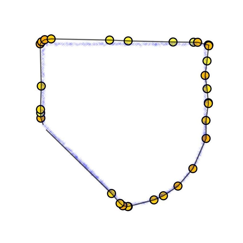
Under review as a conference paper at ICLR 2021

                                                         Figure 7: Distribution of the per-region log-
                                                         determinants (bottom row) for DGN trained on
data
                                                         a bimodal distribution with varying per mode
                                                         variance (first row), demonstrating how the data
                                                         multimodality and concentration pushes the per-
                                                         region determinant of Aω to greatly increase in
# regions

                                                         turn leading to large amplitude layer weights and
                                                         impacting the stability of the DGN learning (also
                                                         recall Lemma 1). Additional experiments are
                                                         given in Fig. 15 in Appendix D.6.

5.1 A NALYTICAL O UTPUT D ENSITY
Given a distribution pz over the latent space, we can explicitly compute the output distribution after
the application of G, which lead to an intuitive result exploiting the piecewise affine property of the
generator; denote by σi (Aω ) the ith singular value of Aω .

Lemma 1. Then,
            p the volume of a region ω ∈ Ω denoted by µ(ω) is related to the volume of G(ω)
                                   Q
by µ(G(ω)) = det(ATω Aω )µ(ω) = i:σi (Aω )>0 σi (Aω )µ(ω).
Theorem 3. The generator probability density pG (x) given pz and a injective generator G with
                                                              p G−1 (x)
per-region inverse G−1                                       √z ( ω T ) 1{x∈G(ω)} .
                                                       P
                    ω from Thm. 4 is given by pG (x) =   ω∈Ω            det(Aω Aω )

That is, the distribution obtained in the output space naturally corresponds to a piecewise affine
transformation of the original latent space distribution, weighted by the change in volume of the
per-region mappings. We derive the analytical form for the case of Gaussian and Uniform latent
distribution in Appendix B. From the analytical derivation of the generator density distribution, we
obtain its differential entropy.

                                            p of the output distribution pG of the DGN is given by
Corollary 1. The differential Shannon entropy
                      P
E(pG ) = E(pz ) + ω∈Ω P (z ∈ ω) log( det(ATω Aω )).
As the result, the differential entropy of the output distribution pG corresponds to the differential
entropy of the latent distribution pz plus a convex combination of the per-region volume change.
It is thus possible to optimize the latent distribution pz to better fit the target distribution entropy
as in Ben-Yosef & Weinshall (2018) and whenever the prior distribution is fixed, any gap between
the latent and output distribution entropy imply the need for high change in volumes between ω
and G(ω). The use of the above results to obtain the analytical form of the density covering the
generative manifold in the Gaussian and Uniform prior cases is done in Appendix B, where we
relate DGN to Kernel Density Estimation (KDE) Rosenblatt (1956) and in particular adaptive KDE
Breiman et al. (1977). We also carefully link DGNs and normalizing flows in Appendix C.
5.2 O N THE D IFFICULTY OF G ENERATING L OW ENTROPY /M ULTIMODAL D ISTRIBUTIONS
We conclude this study by hinting at the possible main cause of instabilities encountered when
training DGNs on multimodal densities or other atypical cases.

We demonstrated in Thm. 3 and Cor. 1 that the product of the nonzero singular values of Aω plays
the central role to concentrate or disperse the density on G(ω). Even when considering the a simple
mixture of Gaussians case, it is clear that the standard deviation of the modes and the inter-mode
distances will put constraints on the singular values of the slope matrix Aω , in turn stressing the
parameters W ` as they compose the slope matrix (see Fig. 10 in the Appendix for details on this
relationship). This problem emerges from the continuous property of DGNs which have to somehow
connect in the output space the different modes. We highlight this in Fig. 7, where we trained a GAN
DGN on two Gaussians for different scaling

In conclusion, the continuity property is a source of the training instabilities while playing a key role
into the DGN interpolation and generalization capacity. Understanding the relationships between the
per-layer parameters, standard regularization techniques, such as Tikhonov, and the multimodality of
the target distribution will thus enable practitioners to find the best compromise to stabilize training
of a continuous DGN that provides sufficient data approximation.

                                                   8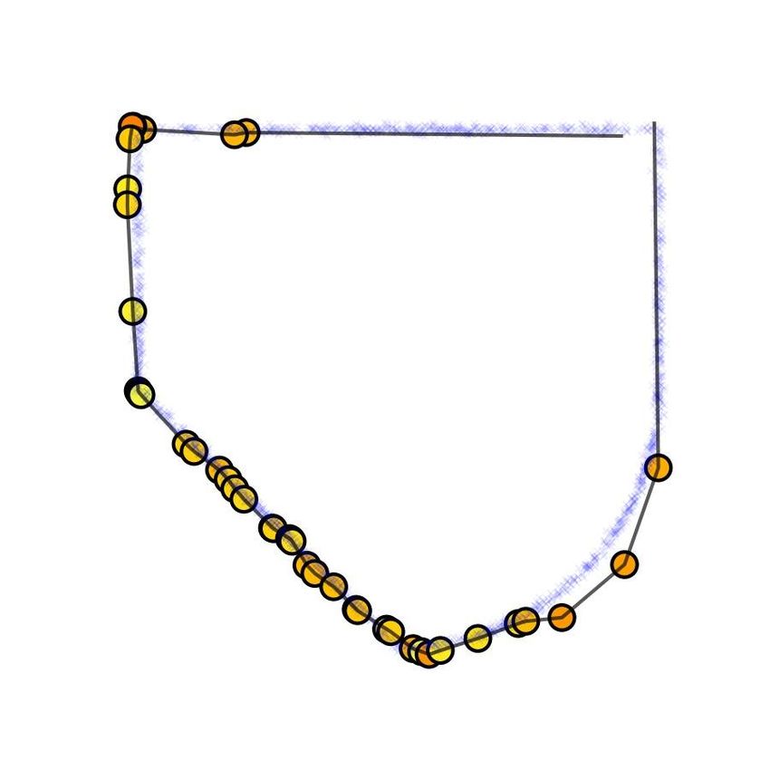
Under review as a conference paper at ICLR 2021

R EFERENCES
Sidney N Afriat. Orthogonal and oblique projectors and the characteristics of pairs of vector spaces.
  In Mathematical Proceedings of the Cambridge Philosophical Society, volume 53, pp. 800–816.
  Cambridge University Press, 1957.
Martin Arjovsky, Soumith Chintala, and Léon Bottou.            Wasserstein gan.     arXiv preprint
 arXiv:1701.07875, 2017.
Philip Bachman, Ouais Alsharif, and Doina Precup. Learning with pseudo-ensembles. In Advances
  in neural information processing systems, pp. 3365–3373, 2014.
Pierre Baldi and Peter J Sadowski. Understanding dropout. In Advances in neural information
  processing systems, pp. 2814–2822, 2013.
R. Balestriero and R. Baraniuk. Mad max: Affine spline insights into deep learning. arXiv preprint
  arXiv:1805.06576, 2018a.
R. Balestriero and R. G. Baraniuk. A spline theory of deep networks. In Proc. Int. Conf. Mach.
  Learn., volume 80, pp. 374–383, Jul. 2018b.
Randall Balestriero and Richard G Baraniuk. From hard to soft: Understanding deep network non-
  linearities via vector quantization and statistical inference. arXiv preprint arXiv:1810.09274,
  2018c.
Randall Balestriero, Romain Cosentino, Behnaam Aazhang, and Richard Baraniuk. The geometry
  of deep networks: Power diagram subdivision. In Advances in Neural Information Processing
  Systems 32, pp. 15806–15815. 2019.
Sudipto Banerjee and Anindya Roy. Linear Algebra and Matrix Analysis for Statistics. Chapman
  and Hall/CRC, 2014.
Matan Ben-Yosef and Daphna Weinshall. Gaussian mixture generative adversarial networks for
 diverse datasets, and the unsupervised clustering of images. arXiv preprint arXiv:1808.10356,
 2018.
Y. Bengio, A. Courville, and P. Vincent. Representation learning: A review and new perspectives.
   IEEE Trans. Pattern Anal. Mach. Intell., 35(8):1798–1828, 2013.
Ake Bjorck and Gene H Golub. Numerical methods for computing angles between linear subspaces.
  Mathematics of computation, 27(123):579–594, 1973.
Piotr Bojanowski, Armand Joulin, David Lopez-Paz, and Arthur Szlam. Optimizing the latent space
  of generative networks. arXiv preprint arXiv:1707.05776, 2017.
Leo Breiman, William Meisel, and Edward Purcell. Variable kernel estimates of multivariate densi-
  ties. Technometrics, 19(2):135–144, 1977.
Joan Bruna and Stéphane Mallat. Invariant scattering convolution networks. IEEE transactions on
  pattern analysis and machine intelligence, 35(8):1872–1886, 2013.
Fred B Bryant and Paul R Yarnold. Principal-components analysis and exploratory and confirmatory
  factor analysis. 1995.
Pierre Comon. Independent Component Analysis, a new Concept? Signal Processing, 36(3):287–
  314, 1994.
Thomas M Cover and Joy A Thomas. Elements of Information Theory. John Wiley & Sons, 2012.
Tim R Davidson, Luca Falorsi, Nicola De Cao, Thomas Kipf, and Jakub M Tomczak. Hyperspheri-
  cal variational auto-encoders. arXiv preprint arXiv:1804.00891, 2018.
Carl De Boor, Carl De Boor, Etats-Unis Mathématicien, Carl De Boor, and Carl De Boor. A practical
  guide to splines, volume 27. springer-verlag New York, 1978.

                                                 9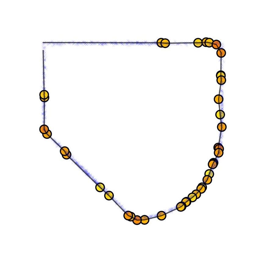
Under review as a conference paper at ICLR 2021

Laurent Dinh, David Krueger, and Yoshua Bengio. Nice: Non-linear independent components esti-
  mation. arXiv preprint arXiv:1410.8516, 2014.
Laurent Dinh, Jascha Sohl-Dickstein, and Samy Bengio. Density estimation using real nvp. arXiv
  preprint arXiv:1605.08803, 2016.
David L Donoho, Iain M Johnstone, et al. Ideal denoising in an orthonormal basis chosen from a
  library of bases. Comptes rendus de l’Académie des sciences. Série I, Mathématique, 319(12):
  1317–1322, 1994.
Ishan Durugkar, Ian Gemp, and Sridhar Mahadevan. Generative multi-adversarial networks. arXiv
   preprint arXiv:1611.01673, 2016.
Gintare Karolina Dziugaite, Daniel M Roy, and Zoubin Ghahramani. Training generative neural
  networks via maximum mean discrepancy optimization. arXiv preprint arXiv:1505.03906, 2015.
Otto Fabius and Joost R van Amersfoort. Variational recurrent auto-encoders. arXiv preprint
  arXiv:1412.6581, 2014.
Xavier Glorot, Antoine Bordes, and Yoshua Bengio. Deep sparse rectifier neural networks. In
  Proceedings of the fourteenth international conference on artificial intelligence and statistics, pp.
  315–323, 2011.
I. Goodfellow, Y. Bengio, and A. Courville. Deep Learning, volume 1. MIT Press, 2016.
I. J Goodfellow, J. Pouget-Abadie, M. Mirza, B. Xu, D. Warde-Farley, S. Ozair, A. Courville, and
   Y. Bengio. Generative adversarial nets. In Proceedings of the 27th International Conference on
   Neural Information Processing Systems, pp. 2672–2680. MIT Press, 2014.
Will Grathwohl, Ricky TQ Chen, Jesse Betterncourt, Ilya Sutskever, and David Duvenaud. Ffjord:
 Free-form continuous dynamics for scalable reversible generative models. arXiv preprint
 arXiv:1810.01367, 2018.
Peter J Green and Bernard W Silverman. Nonparametric regression and generalized linear models:
  a roughness penalty approach. Crc Press, 1993.
Chong Gu. Smoothing spline ANOVA models, volume 297. Springer Science & Business Media,
  2013.
L. A. Hannah and D. B. Dunson. Multivariate convex regression with adaptive partitioning. J. Mach.
   Learn. Res., 14(1):3261–3294, 2013.
Kazuyuki Hara, Daisuke Saitoh, and Hayaru Shouno. Analysis of dropout learning regarded as en-
  semble learning. In International Conference on Artificial Neural Networks, pp. 72–79. Springer,
  2016.
Kaiming He, Xiangyu Zhang, Shaoqing Ren, and Jian Sun. Delving deep into rectifiers: Surpassing
  human-level performance on imagenet classification. In Proceedings of the IEEE international
  conference on computer vision, pp. 1026–1034, 2015.
Irina Higgins, Loic Matthey, Arka Pal, Christopher Burgess, Xavier Glorot, Matthew Botvinick,
   Shakir Mohamed, and Alexander Lerchner. beta-vae: Learning basic visual concepts with a
   constrained variational framework. ICLR, 2(5):6, 2017.
Huaibo Huang, Ran He, Zhenan Sun, Tieniu Tan, et al. Introvae: Introspective variational autoen-
  coders for photographic image synthesis. In Advances in Neural Information Processing systems,
  pp. 52–63, 2018.
Aapo Hyvarinen and Hiroshi Morioka. Unsupervised feature extraction by time-contrastive learning
  and nonlinear ica. In Advances in Neural Information Processing Systems, pp. 3765–3773, 2016.
Phillip Isola, Jun-Yan Zhu, Tinghui Zhou, and Alexei A Efros. Image-to-image translation with
  conditional adversarial networks. In Proceedings of the IEEE Conference on Computer Vision
  and Pattern Recognition, pp. 1125–1134, 2017.

                                                  10
Under review as a conference paper at ICLR 2021
David J Ketchen and Christopher L Shook. The application of cluster analysis in strategic manage-
ment research: an analysis and critique. Strategic management journal, 17(6):441–458, 1996.
Hyunjik Kim and Andriy Mnih. Disentangling by factorising. arXiv preprint arXiv:1802.05983,
2018.
D. P Kingma and M. Welling. Auto-encoding variational bayes. arXiv preprint arXiv:1312.6114,
2013.
Durk P Kingma and Prafulla Dhariwal. Glow: Generative flow with invertible 1x1 convolutions. In
Advances in Neural Information Processing Systems, pp. 10215–10224, 2018.
Claudia Lautensack and Sergei Zuyev. Random laguerre tessellations. Advances in Applied Proba-
bility, 40(3):630–650, 2008. doi: 10.1239/aap/1222868179.
Yuanzhi Li and Yingyu Liang. Learning overparameterized neural networks via stochastic gradient
descent on structured data. In Advances in Neural Information Processing Systems, pp. 8157–
8166, 2018.
Francesco Locatello, Stefan Bauer, Mario Lucic, Gunnar Rätsch, Sylvain Gelly, Bernhard
Schölkopf, and Olivier Bachem. Challenging common assumptions in the unsupervised learn-
ing of disentangled representations. arXiv preprint arXiv:1811.12359, 2018.
Alice Lucas, Michael Iliadis, Rafael Molina, and Aggelos K Katsaggelos. Using deep neural net-
works for inverse problems in imaging: beyond analytical methods. IEEE Signal Processing
Magazine, 35(1):20–36, 2018.
Andrew L Maas, Awni Y Hannun, and Andrew Y Ng. Rectifier nonlinearities improve neural net-
work acoustic models. In Proc. icml, volume 30, pp. 3, 2013.
A. Magnani and S. P. Boyd. Convex piecewise-linear fitting. Optim. Eng., 10(1):1–17, 2009.
Xudong Mao, Qing Li, Haoran Xie, Raymond YK Lau, Zhen Wang, and Stephen Paul Smolley.
Least squares generative adversarial networks. In Proceedings of the IEEE International Confer-
ence on Computer Vision, pp. 2794–2802, 2017.
James Munkres. Topology. Pearson Education, 2014.
JinHyeong Park, Zhenyue Zhang, Hongyuan Zha, and Rangachar Kasturi. Local smoothing for
manifold learning. In Proceedings of the 2004 IEEE Computer Society Conference on Computer
Vision and Pattern Recognition, 2004. CVPR 2004., volume 2, pp. II–II. IEEE, 2004.
Michael Puthawala, Konik Kothari, Matti Lassas, Ivan Dokmanić, and Maarten de Hoop. Globally
injective relu networks. arXiv preprint arXiv:2006.08464, 2020.
Danilo Jimenez Rezende and Shakir Mohamed. Variational inference with normalizing flows. arXiv
preprint arXiv:1505.05770, 2015.
Murray Rosenblatt. Remarks on some nonparametric estimates of a density function. The Annals of
Mathematical Statistics, pp. 832–837, 1956.
Walter Rudin. Real and Complex Analysis. Tata McGraw-hill education, 2006.
Jürgen Schmidhuber. Learning factorial codes by predictability minimization. Neural Computation,
4(6):863–879, 1992.
Alexander Schrijver. Theory of linear and integer programming. John Wiley & Sons, 1998.
Michael Spivak. Calculus on manifolds: a modern approach to classical theorems of advanced
calculus. CRC press, 2018.
Gilbert W Stewart. Error and perturbation bounds for subspaces associated with certain eigenvalue
problems. SIAM review, 15(4):727–764, 1973.
Robert L Thorndike. Who belongs in the family? Psychometrika, 18(4):267–276, 1953.
11Under review as a conference paper at ICLR 2021
Vincent Tjeng, Kai Xiao, and Russ Tedrake. Evaluating robustness of neural networks with mixed
integer programming. arXiv preprint arXiv:1711.07356, 2017.
Jakub M Tomczak and Max Welling. Vae with a vampprior. arXiv preprint arXiv:1705.07120, 2017.
Luan Tran, Xi Yin, and Xiaoming Liu. Disentangled representation learning gan for pose-invariant
face recognition. In Proceedings of the IEEE Conference on Computer Vision and Pattern Recog-
nition, pp. 1415–1424, 2017.
Aaron van den Oord, Oriol Vinyals, et al. Neural discrete representation learning. In Advances in
Neural Information Processing Systems, pp. 6306–6315, 2017.
Stefan Wager, Sida Wang, and Percy S Liang. Dropout training as adaptive regularization. In
Advances in Neural Information Processing systems, pp. 351–359, 2013.
M. B. Wakin, D. L. Donoho, H. Choi, and R. G. Baraniuk. The multiscale structure of non-
differentiable image manifolds. In Proc. Int. Soc. Optical Eng., pp. 59141B1–59141B17, July
2005.
Li Wan, Matthew Zeiler, Sixin Zhang, Yann Le Cun, and Rob Fergus. Regularization of neural
networks using dropconnect. In International Conference on Machine Learning, pp. 1058–1066,
2013.
Shuning Wang and Xusheng Sun. Generalization of hinging hyperplanes. IEEE Transactions on
Information Theory, 51(12):4425–4431, 2005.
Yuedong Wang. Smoothing splines: methods and applications. CRC Press, 2011.
David Warde-Farley, Ian J Goodfellow, Aaron Courville, and Yoshua Bengio. An empirical analysis
of dropout in piecewise linear networks. arXiv preprint arXiv:1312.6197, 2013.
Dingdong Yang, Seunghoon Hong, Yunseok Jang, Tianchen Zhao, and Honglak Lee. Diversity-
sensitive conditional generative adversarial networks, 2019.
Junho Yim, Heechul Jung, ByungIn Yoo, Changkyu Choi, Dusik Park, and Junmo Kim. Rotating
your face using multi-task deep neural network. In Proceedings of the IEEE Conference on
Computer Vision and Pattern Recognition, pp. 676–684, 2015.
Junsong Yin, Dewen Hu, and Zongtan Zhou. Noisy manifold learning using neighborhood smooth-
ing embedding. Pattern Recognition Letters, 29(11):1613–1620, 2008.
Liwen Zhang, Gregory Naitzat, and Lek-Heng Lim. Tropical geometry of deep neural networks.
arXiv preprint arXiv:1805.07091, 2018.
Junbo Zhao, Michael Mathieu, and Yann LeCun. Energy-based generative adversarial network.
arXiv preprint arXiv:1609.03126, 2016.
Shengjia Zhao, Jiaming Song, and Stefano Ermon. Towards deeper understanding of variational
autoencoding models. arXiv preprint arXiv:1702.08658, 2017.
12Under review as a conference paper at ICLR 2021
S UPPLEMENTARY M ATERIAL
The following appendices support the main paper and are organized as follows: Appendix A pro-
vides additional insights that can be gained in the generated surface G by studying its angularity,
that is, how adjacent affine subspaces are aligned with each other. This brings new ways to cap-
ture and probe the “curvature” of the generated surface. Appendix B provides additional details on
the probability distribution leaving on the generated surface while Appendix C provides a careful
bridge between DGNs and Normalizing Flows leveraging the proposed CPA formulation. Lastly,
Appendices D and E provide additional figures and training details for all the experiments that were
studied in the main text, and Appendix F provides the proofs of all the theoretical results.
A G ENERATED M ANIFOLD A NGULARITY
We now study the curvature or angularity of the generated mapping. That is, whenever Se < D, the
per-region affine subspace of adjacent region are continuous, and joint at the region boundaries with
a certain angle that we now characterize.
Definition 1. Two regions ω, ω 0 are adjacent whenever they share part of their boundary as in
ω ∩ ω 0 6= ∅.
The angle between adjacent affine subspace is characterized by means of the greatest principal angle
Afriat (1957); Bjorck & Golub (1973) and denote θ. Denote the per-region projection matrix of the
DGN by P (Aω ) = Aω (ATω Aω )−1 ATω where ATω Aω ∈ RS×S and P (Aω ) ∈ RD×D . We now
assume that dim(G) = Z ensuring that ATω Aω is invertible.1
Theorem 4. The angle between adjacent (recall Def. 1) region mappings θ(G(ω), G(ω 0 )) is given
by sin θ(G(ω), G(ω )) = kP (Aω ) − P (Aω0 )k2 , ∀ω ∈ Ω, ω 0 ∈ adj(ω).
0
Notice that in the special case of S = 1, the angle is given by the cosine similarity between the
vectors Aω and Aω0 of adjacent regions, and when S = D − 1 the angle is given by the cosine
similarity between the normal vectors of the D − 1 subspace spanned by Aω and Aω0 respectively.
We illustrate the angles in a simple case D = 2 and Z = 1 in Fig. 3. It can be seen how a DGN
with few parameters produces angles mainly at the points of curvature of the manifold. We also
provide many additional figures with different training settings in Fig. 11 in the Appendix as well as
repetitions of the same experiment with different random seeds.
We can use the above result to study the distribution of angles of different DGNs with random
weights and study the impact of depth, width, as well Z and D, the latent and output dimensions
respectively. Figure 8 summarizes the distribution of angles for several different settings from which
we observe two key trends. First, as codes of adjacent regions q(ω), q(ω 0 ) share a large number of
their values (see Appendix G for details) the affine parameters Aω and Aω0 of adjacent regions
also benefit from this weight sharing constraining the angles between those regions to be much
smaller than if they were random and independent which favors aggressively large angles. Second,
the distribution moments depend on the ratio S/D rather that those values taken independently. In
particular, as this ratio gets smaller, as the angle distribution becomes bi-modal with an emergence
of high angles making the manifold “flatter” overall except in some parts of the space where high
angularity is present.
The above experiment demonstrates the impact of width and latent space dimension into the angu-
larity of the DGN output manifold and how to pick its architecture based on a priori knowledge of
the target manifold. Under the often-made assumptions that the weights of overparametrized DGN
do not move far from their initialization during training Li & Liang (2018), these results also hint at
the distribution of angles after training.
B D ISTRIBUTIONS
Gaussian Case. We now demonstrate the use of the above derivation by considering practical
examples for which we are able to gain ingights into the DGN data modeling and generation. First,
1
The derivation also applies if dim(G) < Z by replacing Aω with A0ω .
13Under review as a conference paper at ICLR 2021
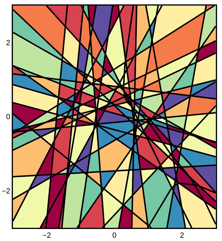
Figure 8: Histograms of the DGN adjacent region angles for DGNs with
two hidden layers, S = 16 and D = 17, D = 32 respectively and vary-
ing width D` on the y-axis. Three trends to observe: increasing the width
increases the bimodality of the distribution while favoring near 0 angles; in-
creasing the output space dimension increases in the number of angles near
orthogonal; the amount of weight sharing between the parameters Aω and
Aω0 of adjacent regions ω and ω 0 makes those distributions much more con-
centrated near 0 than with no weight sharing (depicted in blue), leading to an
overall well behave manifold. Additional figures are available in Fig. 11.
consider that the latent distribution is set as z ∼ N(0, 1) we obtain the following result directly from
Thm. 3.
Corollary 2. The generator density distribution pG (x) given z ∼ N(0, I) is
X e− 21 (x−bω )T (A+ T +
ω ) Aω (x−bω )
pG (x) = p 1{x∈G(ω)} .
ω∈Ω
(2π)S det(ATω Aω )
Proof. First, by applying the above results on the general density formula and setting pz a standard
Normal distribution we obtain that
XZ
1x∈G(ω) pz (G−1 (x)) det(ATω Aω )− 2 dx
1
pG (x ∈ w) =
ω∈Ω ω∩w
XZ 1
1x∈G(ω)
1 −1 2
= p e− 2 kG (x)k2 dx
ω∈Ω ω∩w (2π)S/2 det(ATω Aω )
XZ 1
1x∈G(ω)
1 + T +
= p e− 2 ((Aω (x−bω )) ((A (x−bω )) dx
ω∈Ω ω∩w (2π)S/2 det(ATω Aω )
XZ 1
1x∈G(ω)
1 T + T +
= p e− 2 (x−bω ) (Aω ) Aω (x−bω ) dx
ω∈Ω ω∩w (2π)S/2 T
det(Aω Aω )
giving the desired result.
The above formula is reminiscent of Kernel Density Estimation (KDE) Rosenblatt (1956) and in par-
ticular adaptive KDE Breiman et al. (1977), where a partitioning of the data manifold is performed
on each cell (ω in our case) different kernel parameters are used.
Uniform Case. We now turn into the uniform latent distribution case on a bounded domain U in the
DGN input space. By employing the given formula one can directly obtain that the output density is
given by
1x∈ω det(ATω Aω )− 2
P 1
pG (x) = ω∈Ω (6)
V ol(U )
We can also consider the following question: Suppose we start from a uniform distribution z ∼
U(0, 1) on the hypercube in RS , will the samples be uniformly distributed on the manifold of G?
Proposition 6. Given a uniform latent distribution v ∼ U(0, 1), the sampling of the manifold
G(supp(pz )) will be uniform iff det(ATω Aω ) = c, ∀ω : ω ∩ supp(pz ) 6= ∅, c > 0.
C N ORMALIZING F LOWS AND DGN S
Note from Thm. 3 that we obtain an explicit density distribution. One possibility for learning thus
corresponds to minimizing the negative log-likelihood
q (NLL) between the generator output distribu-
+ T +
p
tion and the data. Recall from Thm. 3 that det ((Aω ) Aω ) = ( det (ATω Aω ))−1 ; thus we can
write the log density from over a sample xn as L(xn ) = log(pz (G−1 (xn )))+log( det(J(xn ))),
p
where J(xn ) = JG−1 (xn )T JG−1 (xn ), J the Jacobian operator. Learning the weights of the DGN
14Under review as a conference paper at ICLR 2021
PN
by minimization of the NLL given by − n=1 L(xn ), corresponds to the normalizing flow model.
The practical difference between this formulation and most NF models comes from having either a
mapping from x 7→ z (NF) or from z 7→ x (DGN case). This change only impacts the speed to
either sample points or to compute the probability of observations. In fact, the forward pass of a
DGN is easily obtained as opposed to its inverse requiring a search over the codes q itself requiring
some optimization. Thus, the DGN formulation will have inefficient training (slow to compute the
likelihood) but fast sampling while NMFs will have efficient training but inefficient sampling.
D E XTRA F IGURES
D.1 D ROPOUT AND DGN S
Figure 9: Reprise of Fig. 4
D.2 E XAMPLE OF D ETERMINANTS
σ1 = 0, σ2 ∈ {1, 2, 3} σ1 = 1, σ2 ∈ {1, 2, 3} σ1 = 2, σ2 ∈ {1, 2, 3}
p
Figure 10: Distribution of log( det(ATω Aω )) for 2000 regions ω with a DGN with L = 3, S = 6, D = 10 and
weights initialized with Xavier; then, half of the weights’ coefficients (picked randomly) are rescaled by σ1 and
the other half by σ2 . We observe that greater variance of the weights increase the spread of the log-determinants
and increase the mean of the distribution.
15Under review as a conference paper at ICLR 2021
D.3 A NGLES H ISTOGRAM
S=2, D=3 S=2, D=4 S=2, D=8 S=4, D=5 S=4, D=8 S=4, D=16
S=8, D=9 S=8, D=16 S=8, D=32 S=16, D=17 S=16, D=32 S=16, D=64
Figure 11: Reproduction of Fig. 8. Histograms of the largest principal angles for DGNs with one
hidden layer (first two rows) and two hidden layers (last two rows). In each case the latent space
dimension and width of the hidden layers is in the top of the column. The observations reinforce the
claims on the role of width and S versus D dimensions.
16Under review as a conference paper at ICLR 2021
D.4 A NGLES M ANIFOLD
Figure 12: The columns represent different widths D` ∈ {6, 8, 16, 32} and the rows correspond to
repetition of the learning for different random initializations of the GDNs for consecutive seeds.
17Under review as a conference paper at ICLR 2021
D.5 M ORE ON MNIST D ISENTANGLEMENT
Figure 13: Randomly generated digits from the trained GAN (top) and trained VAE(bottom) models
for the experiment from Fig. 5. Each row represents a model that was training on a different random
initialization (8 runs in total) which produced the result in Table 1.
18You can also read