MidcurveNN: Neural Network for Computing Midcurve of a Thin Polygon
←
→
Page content transcription
If your browser does not render page correctly, please read the page content below

1154

    MidcurveNN: Neural Network for Computing Midcurve of a Thin Polygon
                                            Yogesh H. Kulkarni1
                                  1
                                      Pune, India, yogeshkulkarni@yahoo.com

                   Corresponding author: Yogesh H. Kulkarni, yogeshkulkarni@yahoo.com

        Abstract. Multiple applications demand lower-dimensional representation of geometric shapes.
        Midsurface is such a two-dimensional (2D) i.e., surface representation of a three-dimensional
        (3D) thin-walled solid shape. It is used in applications such as animation, shape match-
        ing, retrieval, finite element analysis, etc. Similarly, Midcurve is one-dimensional (1D) i.e.,
        a curve representation of a two-dimensional (2D) sketch profile shape. Methods available
        to compute Midcurves vary based on the type of the input shape (images, sketches, etc.)
        and processing (thinning, Medial Axis Transform (MAT), Chordal Axis Transform (CAT),
        Straight Skeletons, etc.).
            This paper talks about a novel method called MidcurveNN which uses Encoder-Decoder
        neural network for computing Midcurve from images of 2D thin polygons in a supervised
        learning manner. This dimension reduction transformation from input 2D thin polygon image
        to output 1D Midcurve image is learnt by the neural network, which can then be used to
        compute Midcurve of an unseen 2D thin polygonal shape.

        Keywords: Midcurve, Encoder-Decoder, Neural Network
        DOI: https://doi.org/10.14733/cadaps.2022.1154-1161

1   INTRODUCTION
Computer-aided Design (CAD) models of thin-walled solids such as sheet metal or plastic parts are often
reduced dimensionally to their corresponding Midsurfaces for quicker and fairly accurate results of Computer-
aided Engineering (CAE) analysis (Figure 1).
    A Midsurface is a surface lying midway of (and representing) the input shape (Figure 2). Computation of
the Midsurface is still a time-consuming and mostly, a manual task due to lack of robust-automated approaches.
Many of the existing automatic Midsurface generation approaches result in some kind of failures such as gaps,
missing patches, overlapping surfaces, etc. It takes hours or even days to correct such errors with manual
intervention. Computing robust Midsurface, thus, is need of the hour.
    As Midsurface is 2D representation of a 3D thin solid, Skeleton (also known as Medial Object, Medial Axis,
Chordal Axis, etc.) is one dimensional representation of either 3D or 2D input shapes. Various mathematical
formulations/approaches used for their generation are Medial Axis Transform (MAT), Chordal Axis Transform
(CAT), Pairing, Thinning, etc. (Figure 3).

                                              Computer-Aided Design & Applications, 19(6), 2022, 1154-1161
                                               © 2022 CAD Solutions, LLC, http://www.cad-journal.net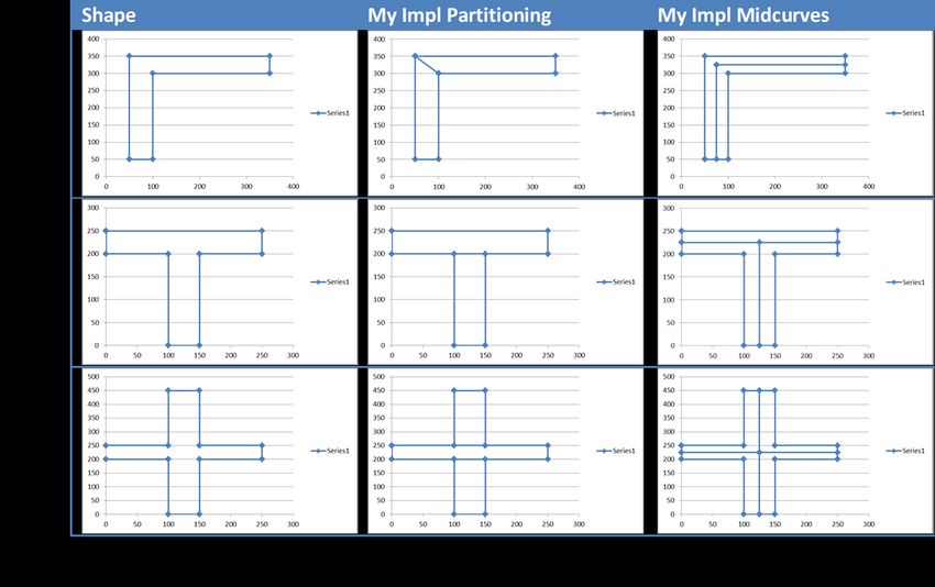
1155

                           Figure 1: Computer-aided PDP (Source: Tierney[2])

                                           Figure 2: Midsurface

                              Figure 3: Medial Object computation methods

    Midcurve is a special case of the Skeleton or MAT (Figure 5b) where the input shape is a 2D profile.
Figure 4 shows that Midcurve lacks the branches and morphologically represents the input shape [6]. MAT
and the input shape are dual (i.e. inter-convertible) whereas Midcurve does not have that requirement.
    Definition: Midcurve is an aggregation of curve segments (where each segment corresponds to a pair of
nonadjacent edges in the object that are closest to each other) that form a closed and connected set and that
satisfy homotopy

                        Figure 4: Medial Axis Transform (MAT) and Midcurve. [6]

                                            Computer-Aided Design & Applications, 19(6), 2022, 1154-1161
                                             © 2022 CAD Solutions, LLC, http://www.cad-journal.net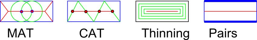
1156

    In CAD, thin solid shapes are typically created by extruding 2D sketch profiles. Thus, generating Midsurface
is same as extruding Midcurve of the profile (Figure 5a).

                          (a)                                                    (b)

                                             Figure 5: Midcurve

    Midcurve, being simpler than the input shape, operations like pattern recognition, approximation, similarity
estimation, collision detection, animation, matching and deformation can be performed efficiently on it rather
than on the input shape.

2   RELATED WORK
Research on computing Midsurface and Midcurve is going on for decades. Figure 6) shows important mile-
stones along the journey. More detailed analysis can be found in the survey paper [3].

                  Figure 6: Milestones along journey of Midsurface computation research

    Following are some salient observations of these classical approaches:
    • Biggest strength of formal approaches like MAT is that it can be computed of any shape, thick or thin.
      Being formally defined, the converse or reversal process, meaning “given a MAT compute the original
      shape”, is possible.

                                             Computer-Aided Design & Applications, 19(6), 2022, 1154-1161
                                              © 2022 CAD Solutions, LLC, http://www.cad-journal.net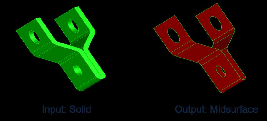
1157

    • Major drawback of MAT, Thinning methods is that it creates unnecessary branches and its shape is
      smaller than the original corresponding faces.
    • MAT based approaches also suffer from robustness problem. A slight change in base geometry forces
      re-computation of MAT and the results could very well be different than the original.
    • Although MAT approaches have been around for decades and are fairly mature, its usage in Midcurve
      generation is still very complex and difficult to ensure appropriate topology.
    • The major limitation of CAT approach is that mesh has to be generated beforehand. Creating con-
      strained, single layer meshes on complicated 2D profiles are, at times, difficult.
    • Thinning approaches are based on split events of the straight line skeleton gives counter-intuitive results
      if the polygon contains sharp reflex vertices.
    • In Pairs approach, the two input curves or surfaces may not be in one-to-one form. In such cases
      maintaining continuity can be challenging.
    • Quality of Midcurve generated by Pairs approach depends on the sampled input shape points.
    • Midcurve by profile decomposition approach is not used widely. The decomposition can result in large
      number of redundant sub-shapes making it ineffective and unstable for further processing.
    The survey paper [3] suggests to avoid formal methods such as MAT, CAD, Thinning and Parametric, for
computing Midcurve as they need heavy post-processing to remove unwanted curves. The heuristic method of
decomposition, has been error prone and inefficient so far. Author’s own past work (Figure 7) demonstrates
reasonable success on simpler shapes, but being rule-based approach, had limitation on scalability.

                       Figure 7: Midcurve Computation by Cellular Decomposition [4]
   Use of Neural Network based techniques have been employed in recent times to compute Skeletons-

                                              Computer-Aided Design & Applications, 19(6), 2022, 1154-1161
                                               © 2022 CAD Solutions, LLC, http://www.cad-journal.net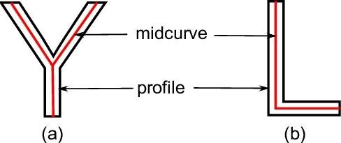
1158

Midcurve, primarily via image processing way. Rodas [7] used Deep Convolutional Neural Networks to compute
object boundary as well as its skeletons, jointly. Shen et. al [9, 8] built Convolutional neural network based
skeleton extractor which is able to capture both local and non-local image context in order to determine the
scale of each skeleton pixel. Zhao [11] used a similar method to [9, 8] but introduced a hierarchical feature
learning mechanism. Wang et. al.[10] introduced content flux in skeletons, which is the learning objective
instead of treating it as a binary classification problem. Approach by Panichev et. al. [5] comes close to the
method proposed here. It used U-net to extract skeletons, but not Midcurve though.
    Review of the state-of-the-art suggests approaches for computing Midcurve are needed to take into account
the application context, accuracy, characteristics and aspect ratio of the sub-polygons. For the present research
work, the Midcurve generation needs primitive shaped, thin sub-polygons. Non-primitive, skewed shapes would
result in inappropriate Midcurves.
    The current paper proposes a novel method of computing Midcurve using Neural Networks i.e Deep
Learning approach.

3   PROPOSED METHOD
The current paper focuses on computing Midcurve for 2D planar sketch profiles and not 3D skeletonal shapes.
Even in 2D profiles, shapes vary enormously. As the first level of simplification, 2D polygons only (with an
assumption that curved shapes can be converted to polygonal shape by faceting) are dealt with. Figure 8
shows some of the input shapes which can be considered. English alphabets are chosen for easy understanding
and verification of the proposed method.

                                     Figure 8: 2D Thin Polygonal shapes

    Computation of Midcurve, in its original form, is transformation of a 2D thin closed, with/without-holes
polygon to 1D open/closed/branched polyline. Paper [4] details one of the effective Midcurve computation
techniques, based on rule-based computational geometry approach. Such techniques have a shortcoming of
not being scalable or generic enough to be able to handle variety of shapes. Deep Learning neural network
architectures show potential of developing such generic models. This dimension reduction transformation
should ideally be modeled as Sequence to Sequence (Seq2Seq) neural architecture, like Machine Translation.

                                              Computer-Aided Design & Applications, 19(6), 2022, 1154-1161
                                               © 2022 CAD Solutions, LLC, http://www.cad-journal.net
1159
Figure 9: Encoder-Decoder Architecture
In the current problem, the input and the output sizes could be different not just in a single sample,
but across all samples. Many current Seq2Seq neural networks need fixed size inputs and outputs, which if
not present in data, are artificially managed by adding padding of certain improbable value. Such padding is
not appropriate for the current Midcurve computation problem, as the padding-value can inappropriately get
treated as part of the valid input. In this initial phase, to circumvent the problem of variable size, image-based
inputs and outputs are used, which are of fixed size. Both input and output polygonal shapes are rasterized
into images of 100x100, thus making them fixed size for all samples, irrespective of the original shapes.
This paper proposes to use such network for Midcurve computation in the form of image-to-image mode.
Input images have thin polygonal shapes whereas output images have corresponding Midcurve images. Figure
9 shows the Encoder-decoder architecture, called MidcurveNN.
Input and output geometries are rasterized into 100x100 size images. Transformations like translation,
rotation and mirroring are applied to create diversity in the samples. MidcurveNN being a Supervised Learning
approach, both input thin-polygons and corresponding output Midcurve polylines are transformed simultane-
ously. Figure 10 shows some samples. This is training data.
Figure 10: Training Data: Inputs (thin polygons) and outputs (Midcurves)
MidcurveNN encoder-decoder has been implemented in Python programming with Keras library [1].
Abridged code listing is presented below (Code Listing 1).
Computer-Aided Design & Applications, 19(6), 2022, 1154-1161
© 2022 CAD Solutions, LLC, http://www.cad-journal.net1160
Listing 1: Encoder-Decoder
input_img = I n p u t ( s h a p e =(input_dim , ) )
e n c o d e d = Dense ( encoding_dim , a c t i v a t i o n= ’ r e l u ’ ) ( input_img )
d e c o d e d = Dense ( input_dim , a c t i v a t i o n= ’ s i g m o i d ’ ) ( e n c o d e d )
a u t o e n c o d e r = Model ( input_img , d e c o d e d )
e n c o d e r = Model ( input_img , e n c o d e d )
e n c o d e d _ i n p u t = I n p u t ( s h a p e =(encoding_dim , ) )
d e c o d e r _ l a y e r = a u t o e n c o d e r . l a y e r s [ −1]
d e c o d e r = Model ( en code d_in put , d e c o d e r _ l a y e r ( e n c o d e d _ i n p u t ) )
a u t o e n c o d e r . compile ( o p t i m i z e r= ’ a d a d e l t a ’ , l o s s= ’ b i n a r y _ c r o s s e n t r o p y ’ )
Encoder takes input image of size 100 × 100 = 10000, then comes Dense layer with size 100 to form the
encoded vector. Decoder takes encoded vector as input, then with a Dense layer expands back to 100 × 100 =
10000 size of the output image. Relu activation is used for Encoder whereas Sigmoid for the decoder. AdaDelta
optimizer with binary cross entropy as loss function is used to compute the losses. Table 1 shows loss across
number of epochs.
Table 1: Improvement in performance with epochs
Epochs Training loss Validation loss
50 -17.6354 -8.3223
200 -16.8878 -7.7672
Some of the results are shown in Figure 11. Inputs are at the top and output Midcurve at the bottom.
Figure 11: Predicted Data: Inputs (thin polygons) and outputs (Midcurves)
Shape on the top is the input thin polygon whereas the corresponding shape at the bottom is the predicted
Midcurve. It can be clearly seen that the network is able to localize the shape and learn the dimension reduction
Computer-Aided Design & Applications, 19(6), 2022, 1154-1161
© 2022 CAD Solutions, LLC, http://www.cad-journal.net1161
function reasonably well. It is still not perfect or usable, as some stray points are still being wrongly classified
as the part of output Midcurve. A better network model and/or post processing is needed to make output
Midcurve practically usable.
4 CONCLUSIONS AND FUTURE WORK
Traditional methods of computing Midcurves are predominantly rules-based and thus, have limitation of not
developing a generic model which will accept any input shape. MidcurveNN, a novel Encoder-Decoder network
attempts to build such a generic model. This paper demonstrates that simple single layer encoder and decoder
network can learn the dimension reduction function reasonably well. Although more development is necessary
in evolving a better neural architecture, the current results show positive potential.
Working on truly variable size inputs (thin polygon) and outputs (polyline) using dynamic graph of Encoder-
Decoder network can be attempted in the future. More and highly diversified data can help improve the quality
of the output. Developing a formal representation of polygonal shapes with variations such as open/closed,
with-without loops, branched as a coherent sequence of points is also on the agenda.
Yogesh H. Kulkarni http://orcid.org/0000-0001-5431-5727
REFERENCES
[1] Chollet, F.: Building autoencoders in keras. https://blog.keras.io/
building-autoencoders-in-keras.html, 2019.
[2] Christopher Tierney, T.R., Declan Nolan; Armstrong, C.: Using mesh-geometry relationships to transfer
analysis models between cae tools. Proceedings of the 22nd International Meshing Roundtable, 2013.
[3] Kulkarni, Y.; Deshpande, S.: Medial object extraction - a state of the art. In International Conference
on Advances in Mechanical Engineering, SVNIT, Surat, 2010.
[4] Kulkarni, Y.; Sahasrabudhe, A.; Kale, M.: Dimension-reduction technique for polygons. International
Journal of Computer Aided Engineering and Technology, 9(1), 2017. http://doi.org/10.1504/
IJCAET.2017.080772.
[5] Panichev, O.; Voloshyna, A.: U-net based convolutional neural network for skeleton extraction. In Pro-
ceedings of the IEEE/CVF Conference on Computer Vision and Pattern Recognition (CVPR) Workshops,
2019.
[6] Ramanathan, M.; Gurumoorthy, B.: Generating the mid-surface of a solid using 2d mat of its
faces. Computer-Aided Design and Applications, 1(1-4), 665–674, 2004. http://doi.org/10.1080/
16864360.2004.10738312.
[7] Rodas, C.B.: Joint object boundary and skeleton detection using convolutional neural networks, 2019.
[8] Shen, W.; Zhao, K.; Jiang, Y.; Wang, Y.; Bai, X.; Yuille, A.: Deepskeleton: Learning multi-task scale-
associated deep side outputs for object skeleton extraction in natural images. IEEE Transactions on
Image Processing, 26(11), 5298–5311, 2017. ISSN 1941-0042. http://doi.org/10.1109/tip.2017.
2735182.
[9] Shen, W.; Zhao, K.; Jiang, Y.; Wang, Y.; Zhang, Z.; Bai, X.: Object skeleton extraction in natural
images by fusing scale-associated deep side outputs, 2016.
[10] Wang, Y.; Xu, Y.; Tsogkas, S.; Bai, X.; Dickinson, S.; Siddiqi, K.: Deepflux for skeletons in the wild,
2018.
[11] Zhao, K.; Shen, W.; Gao, S.; Li, D.; Cheng, M.M.: Hi-fi: Hierarchical feature integration for skeleton
detection, 2018.
Computer-Aided Design & Applications, 19(6), 2022, 1154-1161
© 2022 CAD Solutions, LLC, http://www.cad-journal.netYou can also read