MITIGATION OF GROUND VIBRATIONS BY CIRCULAR ARRAYS OF RIGID BLOCKS
←
→
Page content transcription
If your browser does not render page correctly, please read the page content below
COMPDYN 2019
 7th ECCOMAS Thematic Conference on
 Computational Methods in Structural Dynamics and Earthquake Engineering
 M. Papadrakakis, M. Fragiadakis (eds.)
 Crete, Greece, 24–26 June 2019

 MITIGATION OF GROUND VIBRATIONS BY
 CIRCULAR ARRAYS OF RIGID BLOCKS
 Lars V. Andersen1, Andrew T. Peplow2, and Peter Persson3
 1
 Department of Engineering, Aarhus University
 Inge Lehmanns Gade 10, DK-8000 Aarhus C, Denmark
 e-mail: lva@eng.au.dk
 2
 Department of Natural Sciences and Public Health, Zayed University
 P.O. Box 144534, Abu Dhabi, United Arab Emirates
 e-mail: andrew.peplow@zu.ac.ae
 3
 Department of Construction Sciences, Lund University
 P.O. Box 118, SE-221 00 Lund, Sweden
 e-mail: peter.persson@construction.lth.se

Abstract. Pile driving and other activities in the built environment cause ground vibration at
low frequencies. This may result in annoyance to people as well as damage to civil structures.
It is known that masses added on the ground surface can have an impact on the vibration levels
in the surrounding environment. Hence, employing a semi-analytical model for rigid blocks on
the surface of a layered ground, this paper investigates whether circular arrays of such blocks
can be used as a means of vibration mitigation. The frequency range 0–80 Hz is considered,
since this is relevant to whole-body vibrations of humans as well as the fundamental modes of
resonance in building elements, e.g., floors and walls. Two different soil profiles are analysed:
a soft dry sand layer over a till half-space and a soft wet clay layer over a lime half-space.
Further, three configurations of the block arrays are taken into consideration, and for the first
soil profile also the height of the blocks is varied to test its influence on the insertion loss in a
zone 20–40 m away from the source. The aim is to quantify the overall insertion loss that can
be expected using the proposed methodology. Further, the variation in insertion loss caused by
changes in the block array configuration is examined.

Keywords: Soil, Wave Propagation, Layered Half-Space, Insertion Loss, Wave Impedance.
Lars V. Andersen, Andrew T. Peplow and Peter Persson

1 INTRODUCTION
 Ground vibrations from traffic or construction work may cause damage to structures. They
may as well cause annoyance to inhabitants in urban environments and have an impact on their
health. To reduce the problems associated with ground vibrations, several ideas have been pro-
posed for mitigation. This includes trenches and barriers as well as embedded wave-impeding
blocks (WIBs) or masses placed on the ground surface. These can be placed in front of a vibra-
tion source to prevent vibrations from spreading to the surroundings, or they can be placed in
front of a receiver to protect it, or a combination can be used. In any case, the idea is to insert
one or more obstacles within the wave propagation path that will redirect, reflect or absorb the
waves.
 The literature reports several studies of single blocks or barriers [1, 2, 3] as well as, for
example, double sheet pile walls [4, 5]. Especially, the idea of using blocks placed on the ground
surface for mitigation of ground vibrations was proposed already in the 1970s by Warburton et
al. [7, 8]. Later, Peplow et al. [8] proposed the inclusion of WIBs in the ground, and this concept
was validated experimentally by Masoumi et al. [9].
 To improve the solution that can be achieved with a single barrier or block, arrays of such
barriers and blocks can be introduced. The idea of using structural periodicity to mitigate wave
propagation was originally proposed by Mead [10] who analysed a periodically supported beam.
Recently, Van et al. [11] developed a methodology to design a one-dimensional wave barrier
by topology optimization of a one-dimensional medium. More relevant for the present problem
of ground vibration, Persson et al. [12] studied the effect of having repeated hills and/or valleys,
and Andersen [13] analysed the effect of linear arrays of rigid blocks embedded in the ground
using a two-dimensional model of a periodic structure. This work was extended to three-dimen-
sional analysis of nearly-periodic structures [14, 15, 16]. Furthermore, Peplow et al. [17, 18]
established simplified modelling approach to analysis of linear arrays of blocks placed on the
ground surface. As a common finding of the reported research, periodic inclusions of blocks or
other inhomogeneities have an effect on the ground vibrations and may, if designed properly,
produce band gaps with (almost) no wave propagation.
 As an alternative to the linear barriers or arrays of masses, typically considered, the present
paper proposes the use of circular arrays of rigid blocks. Such arrays can be placed, for example,
around a pile during driving or around a machine foundation—or it can be placed around a
building to partially prevent vibration from reaching it. Only the first scenario is analysed in
the paper, using a semi-analytical model of a layered viscoelastic half-space to represent the
ground. Rigid blocks are placed on the ground surface in concentric circles surrounding the
source point with the aim of reducing the vibration level in a shielded zone 20 m to 40 m from
the centre of the source. A parameter study is performed regarding the number of circles, the
number of blocks in each circle, and the height of the blocks. In any case, the blocks have a
footprint of 1 m by 2 m. It is deemed realistic that such blocks could be produced on a given
site, for example, by filling in steel containers or construction-waste bags with soil that can be
excavated locally. Thus, it is not necessary to place blocks made, for example, of reinforced
concrete that may be difficult and expensive to produce at or move to the site.
 In Section 2, the computational model is described. This includes a description of the semi-
analytical model of the ground and the rigid blocks as well as definition of the various array
configurations. Sections 3 and 4 present two case studies. In Case 1, a soft dry sand layer over
a till half-space is considered, whereas Case 2 concerns a soft wet clay layer over a lime half-
space. These strata are considered to be representative for soil conditions that could typically
cause problems with ground vibrations in the environment surrounding a construction site.
Finally, Section 5 lists the main conclusions of the paper.
Lars V. Andersen, Andrew T. Peplow and Peter Persson

2 COMPUTATIONAL MODEL FOR THE SOIL AND BLOCKS

2.1 Model of a layered ground
 The soil is modelled as a linear viscoelastic solid half-space with surface at 0. In the
time domain and using Cartesian coordinates, the displacement response , , at time
and position , on the ground surface to a surface traction time series , , acting
at the position , can be found as

 , , , , , , d d d , (1)

where , , is the Green’s function for the half-space. This formulation
assumes invariance of the Green’s function to temporal and spatial translation. The latter re-
quires that the half-space is homogenous in the and directions, which in turn requires that
any layers are horizontal. However, even with these constraints, a general analytical expression
for the Green’s function cannot be established in the time–space domain. Instead, a semi-ana-
lytical solution can be obtained by first solving the problem in frequency–horizontal wave-
number domain. Thus, by a triple Fourier transformation, Eq. (1) is reformulated into
 , , ̅ , , , , , (2)
where , , is the triple Fourier transform of , , , , , is the triple
Fourier transform of , , , and ̅ , , is the triple Fourier transform of
 , , . Unlike , , , a closed-form solution exists for ̅ , , in the case
of a horizontally layered linear viscoelastic half-space, as first proposed by Thomson [19] and
Haskell [20], and as further explained in the work by Andersen and Clausen [21]. For a given
combination of wavenumbers and angular frequency, a transfer matrix for a single layer can be
determined in closed form, and the transfer matrices for all layers are then multiplied in order
to obtain a transfer matrix for the layered half-space. This can finally be rearranged into a
Green’s function tensor relating the surface displacement to the surface traction.
 The computational strategy is to discretize the problem into a number of discrete angular
frequencies , 1,2, . . . , . For each frequency, ̅ , , and , , are
evaluated at a number of discrete wavenumbers. Next, double inverse discrete Fourier transfor-
mation is performed with respect to the horizontal wavenumbers. That brings the solution back
into frequency–space domain. Hence, for a given frequency, the displacement , , at
any point on the ground surface due to the traction , , at any point on the surface can
be found. As pointed out by Andersen and Clausen [21], rotational symmetry of the load can
be utilized to speed up the calculations. Further, inverse discrete Fourier transformation can be
used to obtain the time-domain solution. However, the present analyses concern the frequency
domain with focus on the range 0–80 Hz that is relevant to whole-body vibration as well as the
first modes of resonance in typical building structures and soil profiles.
 It is noted that rate-independent material dissipation is assumed in the semi-analytical model
of the ground. Hence, hysteretic damping, represented by the loss factor η, is employed. For
each layer of soil, the material properties are further specified in terms of the shear modulus G,
Poisson’s ratio ν, and the mass density ρ.
 As an example, Figure 1 shows the steady state ground displacement in a model of a layered
soil with 3 m deep soft dry sand overlying a till half-space. Details on the material properties
can be found in Section 3. The load is applied as a uniformly distributed vertical traction over
a circular area with a radius of 1 m, and the displacements are plotted at the frequencies 25 Hz
and 30 Hz, respectively, for the zone up to 40 m away from the centre of the load.

Lars V. Andersen, Andrew T. Peplow and Peter Persson

a) b)
 Figure 1: Snapshots of the steady state ground displacement response to a harmonic vertical load applied
 uniformly over a circular area with radius 1 m: a) Green field at 25 Hz; b) green field at 30 Hz.
 The radius of the model is 40 m and the depth of the model is 12 m.

2.2 Dynamic soil–structure interaction for an array of rigid blocks
 To model the dynamic soil–structure interaction (SSI) for rigid blocks placed on the
ground surface, the interface between each block and the soil is discretized into points. In
the present analyses, rectangular blocks are considered with 6 points in one direction and 12
points in the other direction, i.e. 72. Hence, the total number of soil–structure interaction
points will be 72 . At each of the SSI points, traction is assumed to be dis-
tributed on a small area with rotational symmetry around the point. With reference [21], a so-
called “bell-shaped” traction is applied, i.e. a double Gaussian distribution in the , plane.
Further, load is applied at a source point, adding another three degrees of freedom (d.o.f.) to the
problem, i.e. the discretized ground surface as 3 3 displacement d.o.f.. A global flex-
ibility matrix can now be established, employing the Green’s function
 , , which relates , , to , , . Each of the rigid blocks has six
d.o.f., i.e. a total of 6 rigid-body modes can be identified for the blocks. In addition to this,
the three d.o.f. for the source point must be considered. Thus, one by one, a unit displacement
or rotation is prescribed for each of the 6 3 d.o.f. while fixing the remaining d.o.f. for the
blocks and the load. The displacement components are determined for each of the points
of the local interface between the soil and the block with prescribed unit rigid-body motion.
This provides the matrix , where each column defines one rigid-body mode of a block or the
displacement of the source point in one direction. The magnitude of the traction at each SSI
point due to each unit displacement or rotation can be found as the solution to
 . Finally, for each discrete frequency, a stiffness matrix for the SSI prob-
lem can then be expressed as . This matrix will have the dimensions
 6 3 6 3 .
 Once, the 6 3 rigid-body translations and rotations of the blocks and source point have
been determined for a given load, the displacement at a number of discrete points on the ground
surface can be determined by using the Green’s function. In the present analyses, a circular
zone with radius 40 m is considered, as already discussed in the previous subsection. The dis-
crete points are organized in a regular pattern with a 1.0 m distance in the radial direction and
approximately 1.0 m distance in the azimuthal direction. More precisely, 6 points are placed in
the circle with radius 1 m, 12 points are placed in the circle with radius 2 m, and so on. This
provides a total of 4921 observation points on the ground surface.

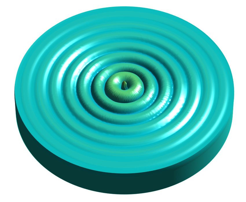
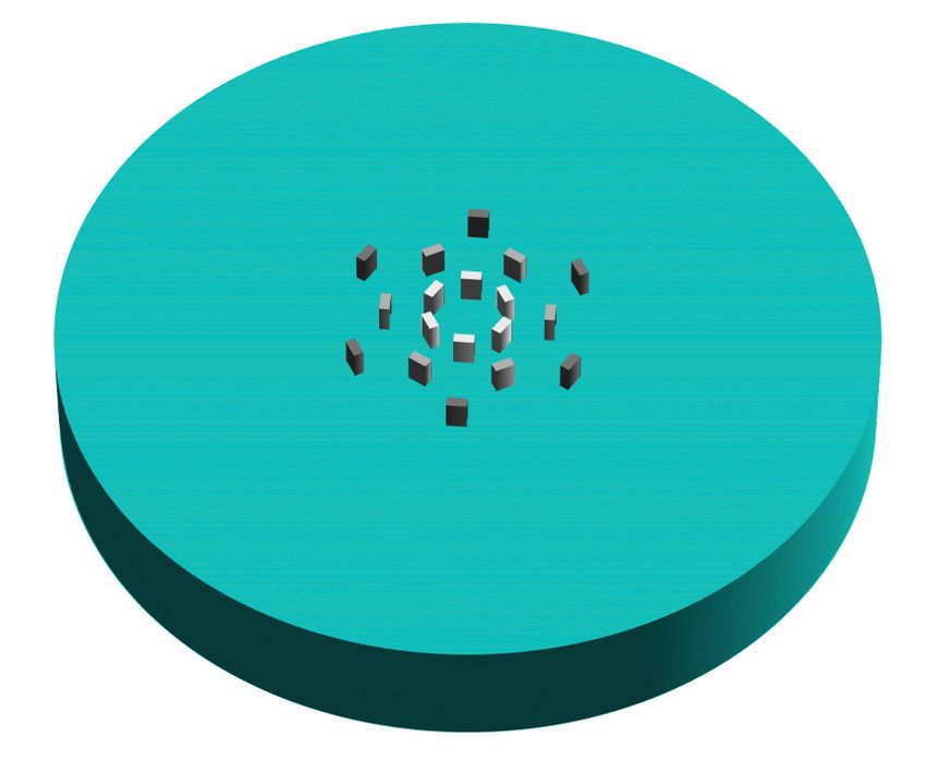
Lars V. Andersen, Andrew T. Peplow and Peter Persson

2.3 Block array configurations
 In order to assess the potential of using circular block arrays to mitigate ground vibration
from a single source on a layered ground, three different overall configurations of the blocks
will be considered. In any case, the blocks are placed on the ground surface in one, two or three
concentric rings with the radii 4 m, 8 m and 12 m, respectively. The radii refer to the distance
between the centre of the loaded circular area and the midpoints of the SSI interfaces between
the individual blocks and the soil. The three configurations are:
a) “Stonehenge” configurations with 6, 12 and 24 blocks in Rings 1, 2 and 3, respectively, cf.
 Figure 2a. The blocks in the inner Ring 1 have the footprint 2 m 1 m with the longer side
 placed tangentially to the perimeter of the circle. The side lengths of the blocks in Rings 2
 and 3 are scaled by a factor of 0.5 / and 0.5 / , respectively, and the height of the blocks
 are scaled by the same factors. Hence, the volume (and hence the mass) of the blocks in Ring
 2 will be one-half compared to that of the blocks in Ring 1, whereas the volume (and mass)
 of the blocks in Ring 3 will be scaled by a factor 0.25. Given that each ring contains twice
 the number of blocks, the total mass of the blocks in each ring is therefore the same.

 a)

b) c)
Figure 2: Three configurations of rigid blocks on the ground surface: a) “Stonehenge” with 6, 12 and 24 blocks
in Rings 1, 2 and 3, respectively; b) “turned rings” with six identical blocks in each ring and Ring 2 turned 30°;
 c) six “linear arrays” with three blocks in each array. The total mass of all blocks in each ring is identical in all
configurations. The radius of the rings are 4 m, 8 m and 12 m, respectively, and the radius of the model is 40 m.
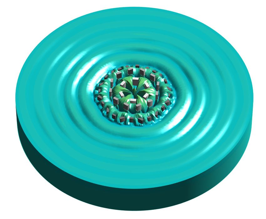
Lars V. Andersen, Andrew T. Peplow and Peter Persson

b) “Turned rings” with six blocks in each ring and with Ring 2 turned by 30° around a vertical
 axis through the load centre relative to Rings 1 and 3, cf. Figure 2b. Thus, when all rings are
 present, the middle ring “closes the gaps” between the blocks in the inner and outer rings. In
 this configuration, the blocks are identical, all having the footprint 2 m 1 m, again with
 the longer side placed tangentially to the perimeter of the circle. Given that six blocks are
 present in each ring, the total mass of the blocks in each ring is therefore again the same.
c) “Linear arrays” with one, two or three blocks lined up along six radii, cf. Figure 2c. Except
 for the relative orientation of Ring 2, this configuration is identical to the “turned rings”.
 The blocks are rigid and have a mass density of 2000 kg/m3. The height of all blocks (in the
inner Ring 1 for the “Stonehenge” configuration” and in all rings for the other configurations)
is either 1 m, 2 m or 3 m. As indicated above, the blocks in Rings 2 and 3 in the “Stonehenge”
configuration will be downscaled to provide the same total mass in each ring.
 Figure 3 shows example results for the “Stonehenge” configuration with three rings of blocks
placed on a soft dry sand layer over a till half-space (the soil properties are given in Section 3).
These results should be compared with the green-field response shown in Figure 1. Clearly, for
the present case, the “Stonehenge” provides excellent mitigation of ground vibrations in the
surrounding environment at the frequency 25 Hz, whereas the effect at 30 Hz is limited.

a) b)
 Figure 3: Snapshots of the steady state ground displacement response to a harmonic vertical load applied
 uniformly over a circular area with radius 1 m: a) “Stonehenge” at 25 Hz; b) “Stonehenge” at 30 Hz.
 The radius of the model is 40 m and the depth of the model is 12 m.

2.4 Calculation of insertion loss and transmission loss in protected zone
 To quantify the effect of block arrays with different configurations on the ground vibration
level in the surrounding environment, the insertion loss (IL) is calculated. For a given position
 , and angular frequency , the IL is determined as the difference in dB in the vibration
levels before and after insertion of the blocks, defining a reduction in vibration level as a posi-
tive insertion loss. For displacement component and block array configuration ,
 , , 20 log , , 20 log , , , (3)
where , , is the displacement amplitude after insertion of the block array, and
 , , is the reference displacement amplitude before insertion of the block array, i.e.
the vibration level in the green field. The present analyses consider vertical vibrations caused
by a unit-magnitude vertical load applied uniformly over a circular area with radius 1 m. Hence,
 , , is calculated at the 4921 observation points on the ground surface.
Lars V. Andersen, Andrew T. Peplow and Peter Persson

 A high value for IL is advantageous. However, array configurations that provide high IL in
frequency ranges with low vibration levels, but low IL in frequency ranges with high vibration
levels, are not effective solutions. Hence, to assess the quality of an array, the reference level
(RL) for vibrations at a given observation point is important. The present analyses employ the
definition:
 , , 20 log , , 20 log , (3)
where , , is the displacement amplitude in the greenfield when a unit-magnitude
(1 N) vertical load is applied, and 1 pm. Again, the vertical vibration level is in focus;
hence, , , is evaluated for the observation points. It should be noted that the present
definition of the RL corresponds to a transfer function for the layered ground. Thus, it contains
no information about the frequency content of a source—it only provides information about the
capacity of the ground to transfer vibration from a position at the surface to another.
 In the following sections, the IL and RL will be determined for two different stratifications
of the soil and for the various configurations of the block arrays described in the previous sub-
section. In order to provide single-value measures of the IL and RL at a given frequency, the
mean values of , , and , , are determined for the donut-shaped zone,
coined here as the “shielded zone” bounded by the two circles with radii 20 m and 40 m, re-
spectively. Further, the 10% and 90% quantiles are calculated in order to quantify the variation
of the quantities within the shielded zone.

3 CASE 1: A SOFT DRY SAND LAYER OVER A HALF-SPACE OF TILL
 The first case concerns a 3 m deep soft dry sand layer overlying a half-space of till. Material
properties for the two soil layers are listed in Table 1. Three subcases are considered: Case 1.1
with 1 m high blocks, Case 1.2 with 2 m high blocks and Case 1.3 with 3 m high blocks.

 Soil layer Shear modulus Poisson’s ratio Mass density Loss factor Thickness
 (from top) G [MPa] ν [-] ρ [kg/m3] η [%] h [m]
 Sand, soft, dry 35.72 0.3330 1553 4.50 3.0
 Till (half-space) 500.0 0.3500 2100 2.00 ∞
 Table 1: Soil properties for Case 1.

3.1 Case 1.1: 1 m high blocks in three configurations
 Table 2 shows the resonance frequencies of the blocks in Rings 1, 2 and 3 for the various
configurations of the 1 m high blocks in Case 1.1. The resonance frequencies are calculated
from the static stiffness of the ground and the inertia of the blocks. With reference to Subsection
2.3, subcases a, b and c refer to the “Stonehenge”, “turned ring” and “linear array” configura-
tions, respectively. Only the vertical rigid-body translation (or heave mode) and the rotation
around the longer main axis of the SSI interface (or pitch mode) of the blocks are considered.
These modes are deemed to be important regarding the interaction with the surface wave prop-
agating away from the source.
 As a first observation, the resonance frequencies are all in the considered frequency range
0–80 Hz, and the pitch mode has a resonance frequency slightly below that of the heave mode.
Further, the smaller blocks in Rings 2 and 3 of the “Stonehenge” configurations (Case 1.1a)
have higher resonance frequencies than the larger blocks in Ring 1. This is expected, since the
SSI areas are reduced less than the volumes, given that the same scaling is applied in all direc-
tions (length, width and height).
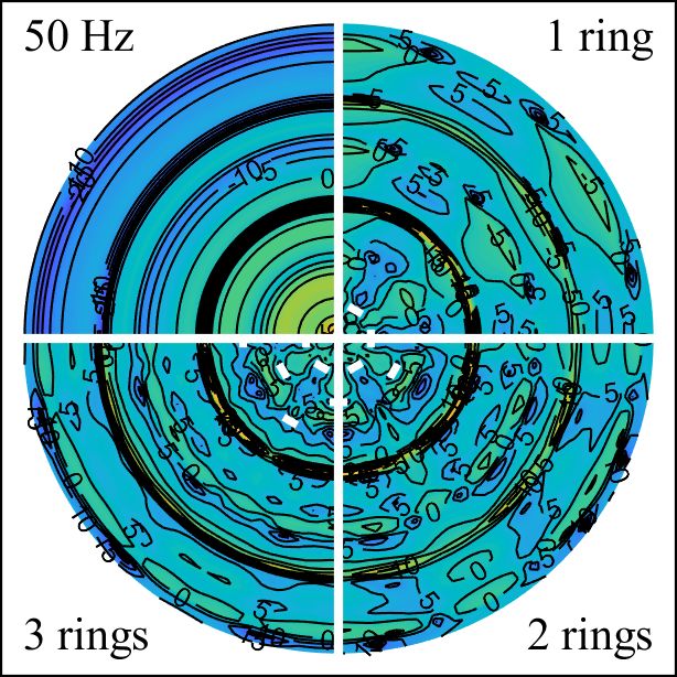
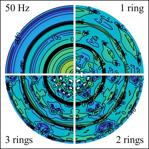
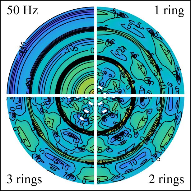
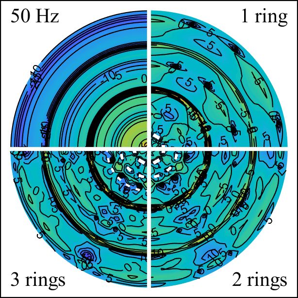
Lars V. Andersen, Andrew T. Peplow and Peter Persson

 Blocks in Ring 1 Blocks in Ring 2 Blocks in Ring 3
 Heave Pitch Heave Pitch Heave Pitch
 Case 1.1a 29.64 19.72 34.27 26.66 40.26 33.20
 Case 1.1b 29.64 19.72 29.60 22.68 29.60 19.70
 Case 1.1c 29.64 19.72 29.60 19.70 29.60 19.70
 Table 2: Resonance frequencies (in Hz) of blocks in Case 1.1.

 Figure 4 shows the mean values of the IL and RL in the shielded zone (20 m to 40 m from
the centre of the load) in Case 1.1a for the frequency range 0–80 Hz and for “Stonehenge”
configurations with either 1, 2 or 3 rings. Figure 5 shows the RL (top left quadrants of the
subplots) and IL (remaining quadrants of the subplots) on the ground surface at nine selected
frequencies. Figure 6 and Figure 7 show similar results for Case 1.1b, the “turned rings”, while
Figure 8 and Figure 9 show the results for Case 1.1c, the “linear arrays”.
 Generally, for Case 1, the RL of vibration in the shielded zone is low for frequencies below
10 Hz, and it increases significantly with an increase of the frequency in the range 10–20 Hz.
This is due to the presence of a cut-on frequency for wave propagation in the sand layer around
12.5 Hz. Below this frequency, the far-field response is dominated by wave propagation in the
much stiffer till half-space, while the soft topsoil only influences the local response near the
source. As the frequency is further increased in the range 20–80 Hz, the mean RL in the shielded
zone decreases. It should be noted that results are presented for the displacement. Obviously,
the frequency dependencies for velocity and acceleration amplitudes are different.
 In terms of the mean IL in the shielded zone, the “Stonehenge” and “turned ring” configu-
rations provide similar results. A small peak in the IL is observed around 22 Hz, and the IL is
generally high, around 10 dB in the frequency range 25–40 Hz. A 5 dB increase of the IL is
achieved by insertion of three rings instead of just one ring. However, by a closer inspection, it
can be observed that Cases 1.1a and 1.1b are different in terms of the variation of the IL within
the shielded zone. For example, at 25 Hz and 30 Hz the “Stonehenge” with 2 rings or 3 rings
provides IL distributions with a high degree of rotational symmetry cf. Figure 5, whereas the
“turned rings” provide more variation in the IL, cf. Figure 7.
 The third configuration, the “linear array” provides a result that is different from the two
other configurations. Thus, Figure 8 shows a significant IL around 22 Hz, which was not the
case for the other configurations. However, around 40 Hz, the IL is low compared to the other
configurations of the block array, and there is almost no gain in IL by inclusion of a second or
third ring. As an interesting observation in Figure 9, it is noted that the linear arrays do not
provide maximum IL in the parts of the shielded zone that lie directly behind the blocks. Due
to wave scattering and interference, the IL at some frequencies is 10–15 dB higher in the gaps
between the linear arrays than just behind the linear arrays.
Lars V. Andersen, Andrew T. Peplow and Peter Persson

 Mean insertion loss [dB]

 Ref. level [dB rel. 1 pm]
Figure 4: Mean insertion loss in dB for the donut-shaped zone between 20 m and 40 m away from the centre of
 the loaded area. Case 1.1a: “Stonehenge” with 1 m high blocks (inner circle) on soft dry sand over till.
 The black line shows the reference level of vibration. Thin lines show 10% and 90% quantiles.

 Figure 5: Contours of the reference vibration levels and insertion losses (in dB) for Case 1.1a, “Stonehenge”
 with 1, 2 and 3 rings. Pale yellow/dark blue shades represent unfavourable/favourable values, respectively.
Lars V. Andersen, Andrew T. Peplow and Peter Persson

 Mean insertion loss [dB]

 Ref. level [dB rel. 1 pm]
Figure 6: Mean insertion loss in dB for the donut-shaped zone between 20 m and 40 m away from the centre of
 the loaded area. Case 1.1b: “Turned rings” with 1 m high blocks (inner circle) on soft dry sand over till.
 The black line shows the reference level of vibration. Thin lines show 10% and 90% quantiles.

 Figure 7: Contours of the reference vibration levels and insertion losses (in dB) for Case 1.1b, “turned rings”
 with 1, 2 and 3 rings. Pale yellow/dark blue shades represent unfavourable/favourable values, respectively.
Lars V. Andersen, Andrew T. Peplow and Peter Persson

 Mean insertion loss [dB]

 Ref. level [dB rel. 1 pm]
Figure 8: Mean insertion loss in dB for the donut-shaped zone between 20 m and 40 m away from the centre of
 the loaded area. Case 1.1c: “Linear arrays” with 1 m high blocks (inner circle) on soft dry sand over till.
 The black line shows the reference level of vibration. Thin lines show 10% and 90% quantiles.

 Figure 9: Contours of the reference vibration levels and insertion losses (in dB) for Case 1.1c, “linear arrays”
 with 1, 2 and 3 rings. Pale yellow/dark blue shades represent unfavourable/favourable values, respectively.
Lars V. Andersen, Andrew T. Peplow and Peter Persson

3.2 Case 1.2: 2 m high blocks in three configurations
 Table 3 shows the resonance frequencies of the blocks in Rings 1, 2 and 3 for the various
configurations of the 2 m high blocks in Case 1.2. Compared with the resonance frequencies
listed in Table 2 (for Case 1.1 with 1 m high block), the values in Table 3 are considerably
lower, especially for the pitch mode. This can be explained by the relatively larger increase of
the rotational inertia compared to the increase of the mass. It can be observed that the resonance
frequency for the pitch mode is now below the cut-on frequency for wave propagation in the
top layer, but the resonance frequencies for the heave mode a closer to the peak of the RL.

 Blocks in Ring 1 Blocks in Ring 2 Blocks in Ring 3
 Heave Pitch Heave Pitch Heave Pitch
 Case 1.2a 20.96 7.562 24.23 9.977 28.47 12.73
 Case 1.2b 20.96 7.562 20.93 9.128 20.93 7.554
 Case 1.2c 20.96 7.562 20.93 7.555 20.93 7.554
 Table 3: Resonance frequencies (in Hz) of blocks in Case 1.2.

 Figure 10 shows the mean values of the IL and RL in the shielded zone (20 m to 40 m from
the centre of the load) in Case 1.2a for the frequency range 0–80 Hz and for “Stonehenge”
configurations with either 1, 2 or 3 rings. Figure 11 shows the RL (top left quadrants of the
subplots) and IL (remaining quadrants of the subplots) on the ground surface at nine selected
frequencies. Figure 12 and Figure 13 show similar results for Case 1.2b, the “turned rings”,
while Figure 14 and Figure 15 show the results for Case 1.2c, the “linear arrays”.
 Compared to Case 1.1, the general observation is that the 2 m high blocks provide signifi-
cantly higher IL than the 1 m high blocks in the frequency range 17–30 Hz. Especially, a very
pronounced peak is present in the mean IL around 18 Hz. The IL at higher frequencies is at the
same time slightly reduced. This results from the lower resonance frequencies of the blocks due
to the increase of inertia when the blocks become higher.
 Little improvement is obtained by including Ring 3 compared to having only two rings.
However, for the “Stonehenge” configuration, the IL in the frequency range 28–35 Hz is in-
creased by about 5 dB by insertion of Ring 3. A smaller gain in the IL, about 2–3 dB, is achieved
in Case 1.2b within the frequency range 23–32 Hz after insertion of the third ring.
 Compared to Cases 1.2b and 1.2c (cf. Figure 12 and Figure 14), the IL is significantly higher
in Case 1.2a (cf. Figure 10) for the configurations with two or three rings in the frequency range
23–33 Hz. Here, the “Stonehenge” configuration provides an IL of about 20 dB, which can be
considered a very large reduction in the vibration level. Furthermore, inspection of Figure 11
shows that the IL is fairly homogeneous, though with variation between 15 dB and 30 dB. There
are no spots with low IL in the shielded zone. For the IL peak near 20 Hz, an even more uniform
distribution of the IL can be observed.
 Finally, comparing Cases 1.2b and 1.2c it can be observed that the “linear arrays” with 2 m
high blocks tend to provide higher IL just behind the arrays at 30 Hz, whereas the IL is on
average higher for the “turned rings”, but with more local variations. This demonstrates that the
orientation of the individual rings can be important in the design of the array, when the goal is
to protect certain smaller zones, rather than the entire larger zone.
Lars V. Andersen, Andrew T. Peplow and Peter Persson

 Mean insertion loss [dB]

 Ref. level [dB rel. 1 pm]
Figure 10: Mean insertion loss in dB for the donut-shaped zone between 20 m and 40 m away from the centre of
 the loaded area. Case 1.2a: “Stonehenge” with 2 m high blocks (inner circle) on soft dry sand over till.
 The black line shows the reference level of vibration. Thin lines show 10% and 90% quantiles.

 Figure 11: Contours of the reference vibration levels and insertion losses (in dB) for Case 1.2a, “Stonehenge”
 with 1, 2 and 3 rings. Pale yellow/dark blue shades represent unfavourable/favourable values, respectively.
Lars V. Andersen, Andrew T. Peplow and Peter Persson

 Mean insertion loss [dB]

 Ref. level [dB rel. 1 pm]
Figure 12: Mean insertion loss in dB for the donut-shaped zone between 20 m and 40 m away from the centre of
 the loaded area. Case 1.2b: “Turned rings” with 2 m high blocks (inner circle) on soft dry sand over till.
 The black line shows the reference level of vibration. Thin lines show 10% and 90% quantiles.

 Figure 13: Contours of the reference vibration levels and insertion losses (in dB) for Case 1.2b, “turned rings”
 with 1, 2 and 3 rings. Pale yellow/dark blue shades represent unfavourable/favourable values, respectively.
Lars V. Andersen, Andrew T. Peplow and Peter Persson

 Mean insertion loss [dB]

 Ref. level [dB rel. 1 pm]
Figure 14: Mean insertion loss in dB for the donut-shaped zone between 20 m and 40 m away from the centre of
 the loaded area. Case 1.2c: “Linear arrays” with 1 m high blocks (inner circle) on soft dry sand over till.
 The black line shows the reference level of vibration. Thin lines show 10% and 90% quantiles.

 Figure 15: Contours of the reference vibration levels and insertion losses (in dB) for Case 1.2c, “linear arrays”
 with 1, 2 and 3 rings. Pale yellow/dark blue shades represent unfavourable/favourable values, respectively.
Lars V. Andersen, Andrew T. Peplow and Peter Persson

3.3 Case 1.3: 3 m high blocks in three configurations
 Table 4 lists the resonance frequencies of the 3 m high blocks in Case 1.3. These are lower
than those in Case 1.2 and even lower than those of Case 1.1. Of particular interest to the present
problem, the resonance frequencies of the 3 m high blocks (for the heave and pitch modes) fall
below 21 Hz where the RL of vibration peaks. Hence, it may be expected that the 3 m high
block will not interact dynamically with the soil to the same extent as the smaller blocks.

 Blocks in Ring 1 Blocks in Ring 2 Blocks in Ring 3
 Heave Pitch Heave Pitch Heave Pitch
 Case 1.3a 17.11 4.185 19.79 5.539 23.25 7.047
 Case 1.3b 17.11 4.185 17.09 5.111 17.09 4.181
 Case 1.3c 17.11 4.185 17.09 4.181 17.09 4.181
 Table 4: Resonance frequencies (in Hz) of blocks in Case 1.3.

 Figure 16 shows the mean values of the IL and RL in the shielded zone (20 m to 40 m from
the centre of the load) in Case 1.3a for the frequency range 0–80 Hz and for “Stonehenge”
configurations with either 1, 2 or 3 rings. Figure 17 shows the RL (top left quadrants of the
subplots) and IL (remaining quadrants of the subplots) on the ground surface at nine selected
frequencies. Figure 18 and Figure 19 show similar results for Case 1.3b, the “turned rings”,
while Figure 20 and Figure 21 show the results for Case 1.3c, the “linear arrays”.
 Comparing Case 1.3 to Case 1.2, the main observation is that the 3 m high blocks perform
poorly compared to the 2 m high blocks. It must be emphasized that this is an observation for
the present configurations of the blocks and for the present stratification of the soil. However,
it cannot be generalized, and in other situations, larger masses may be preferred. Also, increas-
ing the mass by using higher density or increasing the footprint instead of the height may have
a different influence on the result.
 Apart from the lower IL compared to Case 1.2, the “Stonehenge” configuration with two or
three rings (Figure 16 and Figure 17) performs significantly better than the “turned rings” and
“linear arrays” (Figures 18 to 21) in the frequency range 25–30 Hz, whereas the opposite ob-
servation can be made in a narrow range near 16 Hz. Further, at 25 Hz the “Stonehenge” con-
figuration with three rings provide an almost axisymmetric IL distribution in the shielded zone,
whereas the “turned rings” provide a radial (or ray-formed) pattern with very large IL in smaller
zones. Finally, at 25 Hz the “linear array” with three rings provides very low IL. Generally, the
addition of Ring 3 provides very little improvement in Case 1.3c with “linear arrays” of 3 m
high blocks on the soft dry sand layer over the till half-space.
Lars V. Andersen, Andrew T. Peplow and Peter Persson

 Mean insertion loss [dB]

 Ref. level [dB rel. 1 pm]
Figure 16: Mean insertion loss in dB for the donut-shaped zone between 20 m and 40 m away from the centre of
 the loaded area. Case 1.3a: “Stonehenge” with 3 m high blocks (inner circle) on soft dry sand over till.
 The black line shows the reference level of vibration. Thin lines show 10% and 90% quantiles.

 Figure 17: Contours of the reference vibration levels and insertion losses (in dB) for Case 1.3a, “Stonehenge”
 with 1, 2 and 3 rings. Pale yellow/dark blue shades represent unfavourable/favourable values, respectively.
Lars V. Andersen, Andrew T. Peplow and Peter Persson

 Mean insertion loss [dB]

 Ref. level [dB rel. 1 pm]
Figure 18: Mean insertion loss in dB for the donut-shaped zone between 20 m and 40 m away from the centre of
 the loaded area. Case 1.3b: “Turned rings” with 3 m high blocks (inner circle) on soft dry sand over till.
 The black line shows the reference level of vibration. Thin lines show 10% and 90% quantiles.

 Figure 19: Contours of the reference vibration levels and insertion losses (in dB) for Case 1.3b, “turned rings”
 with 1, 2 and 3 rings. Pale yellow/dark blue shades represent unfavourable/favourable values, respectively.
Lars V. Andersen, Andrew T. Peplow and Peter Persson

 Mean insertion loss [dB]

 Ref. level [dB rel. 1 pm]
Figure 20: Mean insertion loss in dB for the donut-shaped zone between 20 m and 40 m away from the centre of
 the loaded area. Case 1.3c: “Linear arrays” with 3 m high blocks (inner circle) on soft dry sand over till.
 The black line shows the reference level of vibration. Thin lines show 10% and 90% quantiles.

 Figure 21: Contours of the reference vibration levels and insertion losses (in dB) for Case 1.3c, “linear arrays”
 with 1, 2 and 3 rings. Pale yellow/dark blue shades represent unfavourable/favourable values, respectively.
Lars V. Andersen, Andrew T. Peplow and Peter Persson

4 CASE 2: A SOFT WET CLAY LAYER OVER A HALF-SPACE OF LIME
 The second case concerns a 5 m deep soft wet clay layer overlying a half-space of lime.
Material properties for the two soil layers are listed in Table 5. The main difference compared
to the previous case, i.e. Case 1, is the larger depth of the top layer combined with the slightly
lower shear modulus. This provides a cut-on frequency of about 7 Hz in Case 2, whereas the
cut-on frequency was around 12.5 Hz in Case 1. Hence, it can be expected that higher mitigation
effect can be obtained by using higher blocks with lower resonance frequencies in this case,
compared to Case 1. Hence, in this section, only results for 3 m high blocks will be discussed.
The resonance frequencies for these blocks are given in Table 6.

 Soil layer Shear modulus Poisson’s ratio Mass density Loss factor Thickness
 (from top) G [MPa] ν [-] ρ [kg/m3] η [%] h [m]
 Sand, soft, dry 30.03 0.4942 1694 4.50 5.0
 Till (half-space) 4300 0.3500 2100 2.00 ∞
 Table 5: Soil properties for Case 2.

 Blocks in Ring 1 Blocks in Ring 2 Blocks in Ring 3
 Heave Pitch Heave Pitch Heave Pitch
 Case 2a 17.85 4.420 20.72 5.854 24.41 7.451
 Case 2b 17.84 4.420 17.81 5.391 17.80 4.415
 Case 2c 17.84 4.420 17.81 4.415 17.80 4.415
 Table 6: Resonance frequencies of blocks in Case 2.

 Figure 22 shows the mean values of the IL and RL in the shielded zone (20 m to 40 m from
the centre of the load) in Case 2a for the frequency range 0–80 Hz and for “Stonehenge” con-
figurations with either 1, 2 or 3 rings. Figure 23 shows the RL (top left quadrants of the subplots)
and IL (remaining quadrants of the subplots) on the ground surface at nine selected frequencies.
Figure 24 and Figure 25 show similar results for Case 2b, the “turned rings”, while Figure 26
and Figure 27 show the results for Case 2c, the “linear arrays”.
 Compared to Case 1, the RL of vibration is lower at frequencies below the cut-on frequency.
This is caused by the higher stiffness of the lime half-space in Case 2 compared to that of the
till half-space in Case 1. However, the peak RL is slightly higher in Case 2 compared to the
peak RL in Case 1, since the clay is slightly softer than the sand.
 For the soil profile considered in Case 2, the various block array configurations mainly pro-
vide mitigation of ground vibrations in the frequency range 12–27 Hz. The “turned rings” have
a good performance around 12–13 Hz and again near 20 Hz. However, outside these narrow
peaks, the IL is low. The “linear arrays” have a similar performance, but the IL in the interme-
diate range 13–18 Hz is better than for the “turned rings”. As can be seen from Figure 25, there
is a clear radial pattern in the IL at 15 Hz for both these configurations.
 The “Stonehenge” configuration is about 5 dB less effective than the other configurations at
frequencies near 12–13 Hz. On the contrary, it provides 10 dB higher IL at frequencies around
25 Hz—however only when all three rings are present. A possible explanation to this is the
somewhat higher resonance frequency of the heave mode for the smaller masses in Ring 3 of
the “Stonehenge” configuration. Whereas the resonance frequency for the larger blocks in the
inner ring, and in all rings of Cases 2b and 2c, are below 20 Hz, the resonance frequency of the
heave mode related to the smaller blocks in Ring 3 of Case 2a is above 24 Hz. Similarly, it can
be seen that the “Stonehenge” with two rings provides slightly higher TL for frequencies just
above 20 Hz, but lower IL at 20 Hz than the array with only one ring.
Lars V. Andersen, Andrew T. Peplow and Peter Persson

 Mean insertion loss [dB]

 Ref. level [dB rel. 1 pm]
Figure 22: Mean insertion loss in dB for the donut-shaped zone between 20 m and 40 m away from the centre of
 the loaded area. Case 2a: “Stonehenge” with 3 m high blocks (inner circle) on soft wet clay over lime.
 The black line shows the reference level of vibration. Thin lines show 10% and 90% quantiles.

 Figure 23: Contours of the reference vibration levels and insertion losses (in dB) for Case 2a, “Stonehenge”
 with 1, 2 and 3 rings. Pale yellow/dark blue shades represent unfavourable/favourable values, respectively.
Lars V. Andersen, Andrew T. Peplow and Peter Persson

 Mean insertion loss [dB]

 Ref. level [dB rel. 1 pm]
Figure 24: Mean insertion loss in dB for the donut-shaped zone between 20 m and 40 m away from the centre of
 the loaded area. Case 2b: “Turned rings” with 3 m high blocks (inner circle) on soft wet clay over lime.
 The black line shows the reference level of vibration. Thin lines show 10% and 90% quantiles.

 Figure 25: Contours of the reference vibration levels and insertion losses (in dB) for Case 2b, “turned rings”
 with 1, 2 and 3 rings. Pale yellow/dark blue shades represent unfavourable/favourable values, respectively.
Lars V. Andersen, Andrew T. Peplow and Peter Persson

 Mean insertion loss [dB]

 Ref. level [dB rel. 1 pm]
Figure 26: Mean insertion loss in dB for the donut-shaped zone between 20 m and 40 m away from the centre of
 the loaded area. Case 2c: “Linear arrays” with 3 m high blocks (inner circle) on soft wet clay over lime.
 The black line shows the reference level of vibration. Thin lines show 10% and 90% quantiles.

 Figure 27: Contours of the reference vibration levels and insertion losses (in dB) for Case 2c, “linear arrays”
 with 1, 2 and 3 rings. Pale yellow/dark blue shades represent unfavourable/favourable values, respectively.
Lars V. Andersen, Andrew T. Peplow and Peter Persson 5 CONCLUSIONS Circular arrays of rigid blocks interacting dynamically with a horizontally layered linear viscoelastic half-space have been analysed. Especially, the mitigation efficiency of such arrays placed around a load acting on the ground surface has been quantified. Two different cases have been considered: Case 1) a soft dry sand layer over a till half-space; Case 2) a soft wet clay layer over a lime half-space. For each case, three different configurations of the circular block arrays have been examined: a) a “Stonehenge” configuration with up to three concentric rings of blocks; b) a “turned rings” configuration with the middle ring turned relatively to the inner and outer ring; c) a “linear array” configuration similar to the “turned rings”, but with all rings oriented in the same way to obtain six rays of linear block arrays. For Case 1, blocks of different heights have been considered. Only 3 m high blocks have been analysed for Case 2. In all the analyses, the frequency range 0–80 Hz has been considered due to its relevance to annoyance caused by whole-body vibration as well as structural damage caused by resonance in the fundamental modes of a building. Results have been presented in terms of the insertion loss that occurs after insertion of one, two or three rings of blocks in each considered combination of soil and array configuration. The mean value of the insertion loss has been calculated for a shielded zone, 20 m to 40 m away from the centre of the circular loaded area. The main conclusions of the paper are as follows: Circular arrays of blocks can have a significant mitigation effect. Insertion losses up to about 20 dB have been observed at frequencies that are relevant to whole-body vibration as well as the first modes of resonance in buildings. In the cases considered in the paper, the circular block arrays have been found to be partic- ularly effective in the frequency range between the cut-on frequency for wave propagation in the soft topsoil layer and up to about 30–40 Hz. This is an important finding, since this is typically the frequency range in which problems with ground vibrations can arise due to the frequency contents of sources—e.g., traffic or pile driving—combined with the ability of the ground to transfer vibrations at different frequencies. The height of the blocks can be adjusted to change the resonance frequencies of the heave and pitch mode. This may be useful in order to calibrate the blocks for optimal performance of the circular arrays in terms of ground vibration mitigation. In many cases, the “Stonehenge” configurations have been found to provide higher insertion losses that the two other configurations of the block arrays. This suggests that combination of blocks with different sizes can be a good alternative to using blocks of equal size. ACKNOWLEDGMENTS The third author gratefully acknowledge the financial support from the Swedish Govern- mental Agency for Innovation Systems (Vinnova), grant ref.no. 2018-04159, as well as from the City of Helsingborg through the call “Plattformen”.
Lars V. Andersen, Andrew T. Peplow and Peter Persson

REFERENCES
[1] L. Andersen and S. R. K. Nielsen, “Reduction of ground vibration by means of barriers
 or soil improvement along a railway track,” Soil Dyn. Earthq. Eng., vol. 25, no. 7–10, pp.
 701–716, Aug. 2005.
[2] D. J. Thompson et al., “Reducing railway-induced ground-borne vibration by using open
 trenches and soft-filled barriers,” Soil Dyn. Earthq. Eng., vol. 88, pp. 45–59, Sep. 2016.
[3] A. Dijckmans et al., “Mitigation of railway induced ground vibration by heavy masses
 next to the track,” Soil Dyn. Earthq. Eng., vol. 75, pp. 158–170, 2015.
[4] L. Andersen and A. H. Augustesen, “Mitigation of traffic-induced ground vibration by
 inclined wave barriers - A three-dimensional numerical analysis,” in 16th International
 Congress on Sound and Vibration 2009, ICSV 2009, 2009, vol. 4.
[5] L. Andersen and M. Liingaard, “Vibration screening with sheet pile walls,” in
 Environmental Vibrations: Prediction, Monitoring, Mitigation and Evaluation (ISEV
 2005), 2005, pp. 429–437.
[6] G. B. Warburton, J. D. Richardson, and J. J. Webster, “Forced Vibrations of Two Masses
 on an Elastic Half Space,” J. Appl. Mech., vol. 38, no. 1, pp. 148–156, 1971.
[7] G. B. Warburton, H. D. Richardson, and J. J. Webster, “Harmonic response of masses on
 an elastic half-space,” J. Eng. Ind. Trans. ASME, vol. 75, pp. 158–170, 1972.
[8] A. T. Peplow, C. J. C. Jones, and M. Petyt, “Surface vibration propagation over a layered
 elastic half-space with an inclusion,” Appl. Acoust., 1999.
[9] H. Masoumi, A. Van Leuven, and S. Urbaniak, “Mitigation of train induced vibrations by
 wave impeding blocks : numerical prediction and experimental validation,” in
 EURODYN 2014, 2014, no. July, pp. 863–870.
[10] D. J. Mead, “Free wave propagation in periodically supported, infinite beams,” J. Sound
 Vib., vol. 11, no. 2, pp. 181–197, 1970.
[11] C. van Hoorickx, O. Sigmund, M. Schevenels, B. S. Lazarov, and G. Lombaert,
 “Topology optimization of two-dimensional elastic wave barriers,” J. Sound Vib., vol.
 376, pp. 95–111, 2016.
[12] P. Persson, K. Persson, and G. Sandberg, “Reduction in ground vibrations by using
 shaped landscapes,” Soil Dyn. Earthq. Eng., vol. 60, pp. 31–43, 2014.
[13] L. V. Andersen, “Using periodicity to mitigate ground vibration,” in COMPDYN 2015 -
 5th ECCOMAS Thematic Conference on Computational Methods in Structural Dynamics
 and Earthquake Engineering, 2015.
[14] L. V. Andersen, P. Bucinskas, P. Persson, M. Muresan, L.-I. Muresan, and I.-O. Paven,
 “Mitigating ground vibration by periodic inclusions and surface structures,” in
 Proceedings of the INTER-NOISE 2016 - 45th International Congress and Exposition on
 Noise Control Engineering: Towards a Quieter Future, 2016, pp. 7469–7480.
[15] L. V. Andersen, A. Peplow, P. Bucinskas, P. Persson, and K. Persson, “Variation in
 models for simple dynamic structure-soil-structure interaction problems,” in Procedia
 Engineering, 2017, vol. 199.
[16] L. V. Andersen, A. Peplow, and P. Bucinskas, “Efficiency of nearly periodic structures
 for mitigation of ground vibration,” in Proceedings of the 6th International Conference
Lars V. Andersen, Andrew T. Peplow and Peter Persson

 on Computational Methods in Structural Dynamics and Earthquake Engineering
 (COMPDYN 2015), 2017, pp. 537–558.
[17] A. Peplow, L. Andersen, and P. Bucinskas, “Variations within simple models for
 structure-soil interaction,” in 24th International Congress on Sound and Vibration, ICSV
 2017, 2017.
[18] A. T. Peplow, L. V. Andersen, and P. Bucinskas, “Environmental vibration reduction
 utilizing an array of mass scatterers,” in Procedia Engineering, 2017, vol. 199.
[19] W. T. Thomson, “Transmission of elastic waves through a stratified solid medium,” J.
 Appl. Phys., vol. 21, no. 2, pp. 89–93, 1950.
[20] N. A. Haskell, “The dispersion of surface waves on multilayered media,” Bull. Seismol.
 Soc. Am., vol. 43, no. 1, pp. 17–34, Jan. 1953.
[21] L. Andersen and J. Clausen, “Impedance of surface footings on layered ground,” Comput.
 Struct., vol. 86, no. 1–2, pp. 72–87, 2008.
You can also read