ML-DSP: Machine Learning with Digital Signal Processing for ultrafast, accurate, and scalable genome classification at all taxonomic levels - bioRxiv
←
→
Page content transcription
If your browser does not render page correctly, please read the page content below
bioRxiv preprint first posted online Aug. 20, 2018; doi: http://dx.doi.org/10.1101/394932. The copyright holder for this preprint
 (which was not peer-reviewed) is the author/funder, who has granted bioRxiv a license to display the preprint in perpetuity.
                                  It is made available under a CC-BY 4.0 International license.
Randhawa et al.

    RESEARCH

ML-DSP: Machine Learning with Digital Signal
Processing for ultrafast, accurate, and scalable
genome classification at all taxonomic levels
Gurjit S. Randhawa1* , Kathleen A. Hill2 and Lila Kari3
*
  Correspondence:
grandha8@uwo.ca                         Abstract
1
  Department of Computer
Science, University of Western          Background: Although methods and software tools abound for the comparison,
Ontario, London, ON, Canada             analysis, identification, and taxonomic classification of the enormous amount of
Full list of author information is
available at the end of the article     genomic sequences that are continuously being produced, taxonomic
                                        classification remains challenging. The difficulty lies within both the magnitude of
                                        the dataset and the intrinsic problems associated with classification. The need
                                        exists for an approach and software tool that addresses the limitations of existing
                                        alignment-based methods, as well as the challenges of recently proposed
                                        alignment-free methods.
                                        Results: We combine supervised Machine Learning with Digital Signal
                                        Processing to design ML-DSP, an alignment-free software tool for ultrafast,
                                        accurate, and scalable genome classification at all taxonomic levels.
                                          We test ML-DSP by classifying 7,396 full mitochondrial genomes from the
                                        kingdom to genus levels, with 98% classification accuracy. Compared with the
                                        alignment-based classification tool MEGA7 (with sequences aligned with either
                                        MUSCLE, or CLUSTALW), ML-DSP has similar accuracy scores while being
                                        significantly faster on two small benchmark datasets (2,250 to 67,600 times
                                        faster for 41 mammalian mitochondrial genomes). ML-DSP also successfully
                                        scales to accurately classify a large dataset of 4,322 complete vertebrate mtDNA
                                        genomes, a task which MEGA7 with MUSCLE or CLUSTALW did not complete
                                        after several hours, and had to be terminated. ML-DSP also outperforms the
                                        alignment-free tool FFP (Feature Frequency Profiles) in terms of both accuracy
                                        and time, being three times faster for the vertebrate mtDNA genomes dataset.
                                        Conclusions: We provide empirical evidence that ML-DSP distinguishes
                                        complete genome sequences at all taxonomic levels. Ultrafast and accurate
                                        taxonomic classification of genomic sequences is predicted to be highly relevant
                                        in the classification of newly discovered organisms, in distinguishing genomic
                                        signatures, in identifying mechanistic determinants of genomic signatures, and in
                                        evaluating genome integrity.
                                        Keywords: Taxonomic classification; Whole genome analysis; Genomic signature;
                                        Alignment-free sequence analysis; Machine learning; Numerical representation of
                                        DNA sequences; Digital Signal Processing; Discrete Fourier Transform

                                      Introduction
                                      Of the estimated existing 8.7 million (±1.3 million) species existing on Earth [1],
                                      only around 1.5 million distinct eukaryotes have been catalogued and classified so
                                      far [2], leaving 86% of existing species on Earth and 91% of marine species still
bioRxiv preprint first posted online Aug. 20, 2018; doi: http://dx.doi.org/10.1101/394932. The copyright holder for this preprint
 (which was not peer-reviewed) is the author/funder, who has granted bioRxiv a license to display the preprint in perpetuity.
                                  It is made available under a CC-BY 4.0 International license.
Randhawa et al.                                                                                                                Page 2 of 23

                 unclassified. To address the grand challenge of all species identification and classifi-
                 cation, a multitude of techniques have been proposed for genomic sequence analysis
                 and comparison. These methods can be broadly classified into alignment-based and
                 alignment-free. Alignment-based methods and software tools are numerous, and in-
                 clude, e.g., MEGA7 [3] with sequence alignment using MUSCLE [4], or CLUSTALW
                 [5, 6]. Though alignment-based methods have been used with significant success for
                 genome classification, they have limitations [7] such as the heavy time/memory
                 computational cost for multiple alignment in multigenome scale sequence data, the
                 need for continuous homologous sequences, and the dependence on a priori assump-
                 tions on, e.g., the gap penalty and threshold values for statistical parameters [8]. In
                 addition, with next-generation sequencing (NGS) playing an increasingly important
                 role, it may not always be possible to align many short reads coming from differ-
                 ent parts of genomes [9]. To address situations where alignment-based methods
                 fail or are insufficient, alignment-free methods have been proposed [10], including
                 approaches based on Chaos Game Representation of DNA sequences [11, 12, 13],
                 random walk [14], graph theory [15], iterated maps [16], information theory [17],
                 category-position-frequency [18], spaced-words frequencies [19], Markov-model [20],
                 thermal melting profiles [21], word analysis [22], among others. Software implemen-
                 tations of alignment-free methods also exist, among them COMET [23], CASTOR
                 [24], SCUEAL [25], REGA [26], KAMERIS [27], and FFP (Feature Frequency Pro-
                 file) [28].

                  While alignment-free methods address some of the issues faced by alignment-based
                 methods, [7] identified the following challenges of alignment-free methods:
                   (i) Lack of software implementation: Most of the existing alignment-free methods
                       are still exploring technical foundations and lack software implementation,
                       which is necessary for methods to be compared on common datasets.
                  (ii) Use of simulated sequences or very small real world datasets: The majority of
                       the existing alignment-free methods are tested using simulated sequences or
                       very small real-world datasets. This makes it hard for experts to pick one tool
                       over the others.
                 (iii) Memory overhead: Scalability to multigenome data can cause memory overhead
                       in word-based methods, specially when long k-mers are used. Information-
                       theory methods address this issue using compression algorithms, but they
                       may fail in identifying complex organization levels in the sequences.

                   In our effort to overcome these challenges, we propose ML-DSP (supervised
                 Machine Learning based on Digital Signal Processing), a general-purpose alignment-
                 free method and software tool for genomic DNA sequence classification at all taxo-
                 nomic levels.

                 Numerical representations of DNA sequences
                 Digital signal processing can be employed in this context because genomic sequences
                 can be numerically represented as discrete numerical sequences and hence treated
                 as digital signals. Several numerical representations of DNA sequences, that use
                 numbers assigned to individual nucleotides, have been proposed in the literature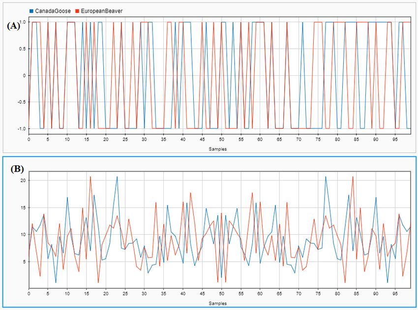
bioRxiv preprint first posted online Aug. 20, 2018; doi: http://dx.doi.org/10.1101/394932. The copyright holder for this preprint
 (which was not peer-reviewed) is the author/funder, who has granted bioRxiv a license to display the preprint in perpetuity.
                                  It is made available under a CC-BY 4.0 International license.
Randhawa et al.                                                                                                                Page 3 of 23

                 [29], e.g., based on a fixed mapping of each nucleotide to a number without bi-
                 ological significance, using mappings of nucleotides to numerical values deduced
                 from their physio-chemical properties, or using numerical values deduced from the
                 doublets or codons that the individual nucleotide was part of [29, 30]. In [31, 32]
                 three physio-chemical based representations of DNA sequences (atomic, molecular
                 mass, and Electron-Ion Interaction Potential, EIIP) were considered for genomic
                 analysis, and the authors concluded that the choice of numerical representation did
                 not have any effect on the results. The latest study comparing different numeri-
                 cal representation techniques [33] concluded that multi-dimensional representations
                 (such as Chaos Game Representation) yielded better genomic comparison results
                 than one-dimensional representations. However, in general there is no agreement on
                 whether or not the choice of numerical representation for DNA sequences makes
                 a difference on the genome comparison results, or what are the numerical repre-
                 sentations that are best suited for analyzing genomic data. We address this issue
                 by providing a comprehensive analysis and comparison of thirteen one-dimensional
                 numerical representations for suitability in genome analysis.

                 Digital Signal Processing
                 Following the choice of a suitable numerical representation for DNA sequences,
                 digital signal processing (DSP) techniques can be applied to the resulting discrete
                 numerical sequences, and the whole process has been termed genomic signal process-
                 ing [30]. DSP techniques have previously been used for DNA sequence comparison,
                 e.g., to distinguish coding regions from non-coding regions [34, 35, 36], to align the
                 genomic signals for classification of biological sequences [37], for whole genome phy-
                 logenetic analysis [38], and to analyze other properties of genomic sequences [39]. In
                 our approach, genomic sequences are represented as discrete numerical sequences,
                 treated as digital signals, transformed via Discrete Fourier Transform into corre-
                 sponding magnitude spectra, and compared via Pearson Correlation Coefficient to
                 create a pairwise distance matrix.

                 Supervised Machine Learning
                 Machine learning has been successfully used in small-scale genomic analysis studies
                 [40, 41, 42]. In this paper we propose a novel combination of supervised machine
                 learning with feature vectors consisting of the distance between the magnitude
                 spectrum of a sequence’s digital signal and the magnitude spectra of all other se-
                 quences in the training set. The taxonomic labels of sequences are provided for
                 training purposes. Six supervised machine learning classifiers (Linear Discriminant,
                 Linear SVM, Quadratic SVM, Fine KNN, Subspace Discriminant, and Subspace
                 KNN) are trained on this pairwise distance vectors, and then used to classify new
                 sequences. Independently, classical multidimensional scaling generates a 3D visu-
                 alization, called Molecular Distance Map (MoDMap) [43], of the interrelationships
                 among all sequences.

                  For our computational experiments, we used a large dataset of 7, 396 complete
                 mtDNA sequences, and six different classifiers, to compare one-dimensional nu-
                 merical representations for DNA sequences used in the literature for classification
bioRxiv preprint first posted online Aug. 20, 2018; doi: http://dx.doi.org/10.1101/394932. The copyright holder for this preprint
(which was not peer-reviewed) is the author/funder, who has granted bioRxiv a license to display the preprint in perpetuity.
It is made available under a CC-BY 4.0 International license.
Randhawa et al. Page 4 of 23
purposes. For this dataset, we concluded that the Purine/Pyrimidine (PP), Real,
and Just-A numerical representations were the top three performers. We analyzed
the performance of ML-DSP in classifying the aforementioned genomic mtDNA se-
quences, from the highest level (domain into kingdoms) to lower level (family into
genera) taxonomical ranks. The average classification accuracy of the ML-DSP was
98% when using the PP, Real, and Just-A numerical representations.
To evaluate our method, we compared its performance (accuracy and speed) on
three datasets: two previously used small benchmark datasets [44], and a large real
world dataset of 4, 322 complete vertebrate mtDNA sequences. We found that ML-
DSP had significantly better accuracy scores than the alignment-free method FFP
on the two small benchmark datasets, while having similar accuracy but better run-
ning time on the large benchmark dataset. When compared to the state-of-the-art
alignment-based method MEGA7, with alignment using MUSCLE or CLUSTALW,
ML-DSP achieved similar accuracy but superior processing times (2,250 to 67,600
times faster) for the small benchmark dataset of 41 mammalian genomes. For the
large dataset, ML-DSP took 28 seconds, while MEGA7(MUSCLE/CLUSTALW)
could not complete the computation after 2 hours/6 hours, and had to be termi-
nated.
Results and Discussion
Following the design and implementation of the ML-DSP genomic sequence classifi-
cation tool prototype, we investigated which type of length-normalization and which
type of distance were most suitable for genome classification using this method. We
then conducted a comprehensive analysis of the various numerical representations
of DNA sequences used in the literature, and determined the top three perform-
ers. Having set these three parameters (length-normalization method, distance, and
numerical representation), we tested ML-DSP’s ability to classify mtDNA genomes
at taxonomic levels ranging from the domain level down to the genus level, and
obtained average levels of classification accuracy of 98%. Finally, we compared ML-
DSP with other alignment-based and alignment-free genome classification methods,
and showed that ML-DSP achieved higher accuracy and significantly higher speeds.
Analysis of distances and of length normalization approaches
To decide which distance measure and which length normalization method were
most suitable for genome comparisons with ML-DSP, we used nine different sub-
sets of full mtDNA sequences from our dataset. These subsets were selected to
include most of the available complete mtDNA genomes (Vertebrates dataset of
4,322 mtDNA sequences), as well as subsets containing similar sequences, of sim-
ilar length (Primates dataset of 148 mtDNA sequences), and subsets containing
mtDNA genomes showing large differences in length (Plants dataset of 174 mtDNA
sequences).
The classification accuracy scores obtained using the two considered distance mea-
sures (Euclidean and Pearson Correlation Coeffient, PCC) and two different length-
normalization approaches (normalization to maximum length and normalization to
median length) on several datasets are listed in Table 1. The classification accuracy
scores are similar, which indicates that the choice of Euclidean or PCC, and thebioRxiv preprint first posted online Aug. 20, 2018; doi: http://dx.doi.org/10.1101/394932. The copyright holder for this preprint
(which was not peer-reviewed) is the author/funder, who has granted bioRxiv a license to display the preprint in perpetuity.
It is made available under a CC-BY 4.0 International license.
Randhawa et al. Page 5 of 23
Table 1 Maximum classification accuracy scores when using Euclidean vs. Pearson’s
correlation coefficient (PCC) as a distance measure.
Max Min Median Maximum Accuracy
No. of
Data Set Length Length Length Euclidean PCC
Seq.
(bp) (bp) (bp) Norm. Norm. Norm. Norm.
to Max to Median to Max to Median
Length Length Length Length
(a) (b) (c) (d)
Primates
148 17531 15467 16554 100% 100% 100% 100%
(Haplorrhini: 115, Strepsirrhini: 33)
Protists
(Alveolata: 34, Rhodophyta: 46, 159 77356 5882 35660 93.7% 93.7% 96.9% 96.9%
Stramenopiles: 79)
Fungi
(Basidiomycota: 30, Pezizomycotina: 104, 226 235849 1364 39154 85.3% 87.5% 88.8% 91.1%
Saccharomycotina:92)
Plants
174 1999595 12998 128211 94.3% 96.0% 93.7% 93.1%
(Chlorophyta: 44, Streptophyta: 130)
Amphibians
290 28757 15757 17271 99.0% 99.0% 98.6% 99.3%
(Anura: 161, Caudata:95, Gymnophiona: 34)
Mammals
(Xenarthrans: 30, Bats: 54,
Carnivores: 135, Even-toed Ungulates: 242, 830 17734 15289 16537 99.3% 99.4% 98.9% 99.0%
Insectivores: 40, Marsupials: 34,
Primates: 148, Rodents and Rabbits: 147)
Insects
(Coleoptera: 95, Dictyptera: 77,
Diptera: 149, Hemiptera: 126, 898 20731 10662 15529 96.3% 97.1% 96.1% 97.0%
Hymenoptera: 47, Lepidoptera:294,
Orthoptera: 110)
3 classes
2170 28757 8118 16361 99.9% 99.8% 99.8% 99.8%
(Amphibians: 290, Mammals: 874, Insects: 1006)
Vertebrates
(Amphibians: 290, Birds: 553, Fish: 2313, 4322 28757 14935 16616 99.5% 99.7% 99.5% 99.6%
Mammals: 874, Reptiles: 292)
Table Average Accuracy —— —— —— —— 96.4% 96.9% 96.9% 97.3%
(a)(c) Genomes normalized to the maximum genome sequence length; (b)(d) Genomes normalized to
the median genome sequence length
choice of one of the above length-normalization approaches do not result in a large
difference in accuracy scores.
In the remainder of this paper we chose the Pearson Correlation Coefficient PCC
because it is scale independent (unlike the Euclidean distance, which is, e.g., sen-
sitive to the offset of the signal, whereby signals with the same shape but different
starting points are regarded as dissimilar [45]), and the length-normalization to
median length because it is economic in terms of memory usage.
Analysis of various numerical representations of DNA sequences
We analyzed the effect on the classification accuracy of ML-DSP of the use of each
of thirteen different one-dimensional numeric representations for DNA sequences,
grouped as: Fixed mappings DNA numerical representations (rows 1, 2, 3, 6, 7,
10, 11, 12, 13, in Table 2), mappings based on some physio-chemical properties of
nucleotides (rows 4, 5, in Table 2), and mappings based on the nearest-neighbour
values (rows 8, 9, in Table 2).
The datasets used for this analysis were the same as those in Table 1. The super-
vised machine learning classifiers used for this analysis were the six classifiers listed
in the Methods section, with the exception of the datasets with more than 2,000
sequences where two of the classifiers (Subspace Discriminant and Subspace KNN)
were omitted as being too slow. The results and the average accuracy scores for all
these numerical representations, classifiers and datasets are summarized in Table 3.
As can be observed from Table 3, for all numerical representations, the table
average accuracy scores (last row: average of averages, first over the six classifiers
for each dataset, and then over all datasets), are high. Surprisingly, even using a
single nucleotide numerical representation, which treats three of the nucleotides as
being the same, and singles out only one of them (Just-A), results in an averagebioRxiv preprint first posted online Aug. 20, 2018; doi: http://dx.doi.org/10.1101/394932. The copyright holder for this preprint
(which was not peer-reviewed) is the author/funder, who has granted bioRxiv a license to display the preprint in perpetuity.
It is made available under a CC-BY 4.0 International license.
Randhawa et al. Page 6 of 23
Table 2 Numerical representations of DNA sequences.
Representation Rules Output for S1 = CGAT
1 Integer T = 0, C = 1, A = 2, G = 3 [1 3 2 0]
2 Integer (other variant) T = 1, C = 2, A = 3, G = 4 [2 4 3 1]
3 Real T = −1.5, C = 0.5, A = 1.5, G = −0.5 [0.5 − 0.5 1.5 − 1.5]
4 Atomic T = 6, C = 58, A = 70, G = 78 [58 78 70 6]
5 EIIP (electron-ion interaction potential) T = 0.1335, C = 0.1340, A = 0.1260, G = 0.0806 [0.1340 0.8060 0.1260 0.1335]
6 PP (purine/pyrimidine) T /C = 1, A/G = −1 [1 − 1 − 1 1]
7 Paired numeric T /A = 1, C/G = −1 [−1 − 1 1 1]
8 Nearest-neighbor based doublet 0 − 15 for all possible doublets [14 8 1 7]
9 Codon 0 − 63 for all possible 64 Codons [2 35 22 44]
10 Just-A A = 1, rest = 0 [0 0 1 0]
11 Just-C C = 1, rest = 0 [1 0 0 0]
12 Just-G G = 1, rest = 0 [0 1 0 0]
13 Just-T T = 1, rest = 0 [0 0 0 1]
Numerical representations of DNA sequences analyzed for usability in genomic classification with
ML-DSP. The second column lists the numerical representation name, the third column describes the
rule it uses, and the fourth is the output of this rule for the input DNA sequence S1 = CGAT . For
the nearest-neighbor based doublet representation and codon representation, the DNA sequence is
considered to be wrapped (the last position is followed by the first).
accuracy of 93.3%. The best accuracy, for these datasets, is achieved when using
the Purine/Pyrimidine (PP) representation, which yields an average accuracy of
95.2%.
For several of the numerical representations the average classification accuracies
are so close that one could not choose a clear winner. For subsequent experiments
we selected the top three representations in terms of accuracy scores: PP, Real and
Just-A numerical representations.
ML-DSP for three classes of vertebrates
As an application of ML-DSP using the Purine/Pyrimidine numerical representation
for DNA sequences, we analyzed the set of vertebrate mtDNA genomes (median
length 16,606 bp). The MoDMap, i.e., the multi-dimensional scaling 3D visualization
of the genome interrelationships as described by the distances in the distance matrix,
is illustrated in Fig 1. The dataset contains 3,740 complete mtDNA genomes: 553
bird genomes, 2,313 fish genomes, and 874 mammalian genomes. Quantitatively, the
classification accuracy score obtained by the Quadratic SVM classifier was 100%.
Classifying genomes with ML-DSP, at all taxonomic levels
We tested the ability of ML-DSP to classify complete mtDNA sequences at various
taxonomic levels. For every dataset, we tested using the PP, Real, and Just-A
numerical representations.
The starting point was domain Eukaryota (7, 396 sequences), which was classified
into kingdoms, then kingdom Animalia was classified into phyla, etc. At each level,
we picked the cluster with the highest number of sequences and then classified it
into the next taxonomic level sub-clusters. The lowest level classified was family
Cyprinidae (81 sequences) into its six genera. The maximum classification accuracy
scores among the six classifiers, for the different taxonomic levels are shown in the
Table 4.
Note that, at each taxonomic level, the maximum classification accuracy scores
(among the six classifiers) for each of the three numerical representations consid-
ered are high, ranging from 92.6% to 100%, with only three scores under 95%. As
this analysis also did not reveal a clear winner among the top three numerical rep-
resentations, the question then arose whether the numerical representation we usebioRxiv preprint first posted online Aug. 20, 2018; doi: http://dx.doi.org/10.1101/394932. The copyright holder for this preprint
(which was not peer-reviewed) is the author/funder, who has granted bioRxiv a license to display the preprint in perpetuity.
It is made available under a CC-BY 4.0 International license.
Randhawa et al. Page 7 of 23
Table 3 Average classification accuracies for 13 numerical representations.
DataSet/ Numerical Representation
Classification NN
Integer Paired
Model Integer Real Atomic EIIP PP based Codon Just-A Just-C Just-G Just-T
(Other) Num.
doublet
Primates (148 sequences)
Linear
98.0% 97.3% 99.3% 96.6% 97.3% 100% 99.3% 99.3% 98.0% 98.0% 99.3% 94.6% 98.0%
Discriminant
Linear SVM 98.6% 98.0% 98.6% 96.6% 97.3% 98.6% 98.6% 98.6% 98.6% 98.6% 98.0% 98.0% 98.0%
Quadratic SVM 98.0% 96.6% 100% 94.6% 93.9% 100% 98.6% 99.3% 98.0% 99.3% 99.3% 98.6% 98.0%
Fine KNN 97.3% 98.0% 100% 97.3% 95.9% 100% 100% 98.6% 98.6% 100% 99.3% 99.3% 98.6%
Subspace
98.6% 100% 99.3% 97.3% 98.0% 98.6% 98.6% 98.6% 98.6% 99.3% 97.3% 99.3% 98.0%
Discriminant
Subspace KNN 97.3% 96.6% 100% 97.3% 95.9% 100% 100% 98.0% 98.0% 98.6% 98.6% 99.3% 97.3%
Average 98.0% 97.8% 99.5% 96.6% 96.4% 99.5% 99.2% 98.7% 98.3% 99.0% 98.6% 98.2% 98.0%
Protists (159 sequences)
Linear
78.0% 81.8% 76.7% 83.0% 82.4% 81.8% 74.2% 83.0% 88.7% 84.3% 75.5% 81.8% 86.8%
Discriminant
Linear SVM 83.6% 82.4% 93.7% 82.4% 82.4% 96.9% 83.6% 83.0% 82.4% 83.6% 83.0% 83.0% 83.0%
Quadratic SVM 86.2% 86.2% 94.3% 83.6% 83.0% 96.2% 86.2% 86.2% 86.2% 85.5% 83.6% 83.6% 86.8%
Fine KNN 88.1% 88.1% 80.5% 84.3% 87.4% 81.8% 90.6% 88.7% 90.6% 89.3% 89.3% 94.3% 89.3%
Subspace
88.1% 87.4% 96.9% 86.8% 88.7% 96.2% 86.8% 85.5% 88.1% 88.7% 91.8% 91.8% 87.4%
Discriminant
Subspace KNN 89.9% 88.1% 94.3% 84.3% 87.4% 95.6% 91.2% 89.9% 91.8% 89.9% 93.1% 93.7% 93.1%
Average 85.7% 85.7% 89.4% 84.1% 85.2% 91.4% 85.4% 86.1% 88.0% 86.9% 86.1% 88.0% 87.7%
Fungi (226 sequences)
Linear
79.0% 79.9% 84.8% 58.0% 64.3% 83.0% 69.2% 64.3% 77.7% 82.6% 73.2% 71.4% 81.7%
Discriminant
Linear SVM 72.8% 63.4% 87.9% 50.4% 49.6% 87.5% 76.8% 64.7% 71.4% 78.6% 69.2% 68.8% 78.6%
Quadratic SVM 58.9% 60.7% 88.4% 54.4% 58.4% 89.7% 74.1% 70.5% 67.9% 69.6% 72.3% 74.1% 62.9%
Fine KNN 61.2% 57.1% 75.0% 54.0% 57.1% 72.3% 75.0% 68.3% 58.9% 71.0% 60.3% 67.0% 67.4%
Subspace
84.8% 82.6% 87.1% 61.6% 62.9% 89.3% 77.7% 68.8% 82.1% 84.8% 74.6% 77.7% 83.9%
Discriminant
Subspace KNN 66.1% 58.9% 91.5% 56.3% 59.4% 91.1% 70.5% 66.5% 62.1% 70.1% 67.9% 75.9% 67.0%
Average 70.5% 67.1% 85.8% 55.8% 58.6% 85.5% 73.9% 67.2% 70.0% 76.1% 69.6% 72.5% 73.6%
Plants (174 sequences)
Linear
94.3% 93.1% 87.4% 91.4% 92.0% 92.0% 91.4% 91.4% 93.7% 94.8% 95.4% 93.7% 95.4%
Discriminant
Linear SVM 96.0% 96.0% 90.2% 96.0% 96.0% 89.1% 96.0% 96.0% 96.0% 96.0% 96.0% 96.0% 96.0%
Quadratic SVM 96.0% 96.0% 92.5% 96.0% 96.0% 90.2% 96.0% 96.0% 96.0% 96.0% 96.0% 96.0% 96.0%
Fine KNN 93.7% 93.7% 85.6% 93.7% 93.7% 85.1% 90.8% 93.1% 93.7% 94.8% 92.5% 92.0% 92.5%
Subspace
94.8% 95.4% 92.5% 93.7% 92.5% 92.5% 95.4% 93.1% 94.8% 94.8% 95.4% 94.3% 96.0%
Discriminant
Subspace KNN 93.7% 93.7% 91.4% 94.3% 93.7% 93.1% 95.4% 93.7% 94.3% 94.8% 94.8% 94.3% 94.8%
Average 94.8% 94.7% 89.9% 94.2% 94.0% 90.3% 94.2% 93.9% 94.8% 95.2% 95.0% 94.4% 95.1%
Amphibians (290 sequences)
Linear
96.6% 93.8% 96.6% 88.6% 93.1% 97.9% 97.9% 96.6% 93.1% 98.3% 97.9% 99.0% 97.2%
Discriminant
Linear SVM 91.4% 90.3% 97.6% 88.6% 89.3% 98.6% 94.8% 94.1% 90.3% 94.1% 94.8% 96.2% 92.1%
Quadratic SVM 92.1% 89.7% 98.3% 66.9% 77.2% 99.3% 97.6% 94.5% 88.3% 96.6% 94.8% 97.9% 94.5%
Fine KNN 91.0% 88.6% 97.6% 85.2% 86.2% 97.9% 92.1% 93.8% 91.0% 95.2% 93.8% 95.9% 92.4%
Subspace
96.2% 93.1% 98.3% 88.6% 91.0% 99.3% 97.6% 97.2% 92.8% 97.2% 97.2% 97.6% 94.8%
Discriminant
Subspace KNN 91.0% 88.3% 97.9% 85.5% 86.6% 98.6% 92.4% 94.1% 89.3% 95.5% 94.1% 95.9% 92.1%
Average 93.1% 90.6% 97.7% 83.9% 87.2% 98.6% 95.4% 95.1% 90.8% 96.2% 95.4% 97.1% 93.9%
Mammals (830 sequences)
Linear
98.2% 98.2% 96.6% 98.0% 97.1% 96.6% 96.9% 97.5% 97.1% 97.8% 97.5% 96.6% 96.4%
Discriminant
Linear SVM 96.0% 93.5% 95.9% 87.8% 88.9% 97.5% 96.0% 94.9% 93.5% 97.7% 97.1% 95.2% 96.4%
Quadratic SVM 94.9% 92.4% 97.6% 52.8% 58.8% 98.0% 97.7% 95.8% 92.9% 97.1% 97.7% 96.5% 96.0%
Fine KNN 94.1% 93.1% 97.6% 80.6% 81.7% 97.8% 96.7% 95.2% 92.8% 97.3% 97.1% 95.9% 96.0%
Subspace
98.7% 99.0% 98.8% 98.0% 97.1% 99.0% 98.1% 98.0% 98.1% 98.7% 98.7% 97.6% 97.8%
Discriminant
Subspace KNN 93.7% 93.3% 98.0% 79.6% 82.4% 98.1% 94.0% 94.6% 92.3% 95.5% 96.4% 96.0% 94.3%
Average 95.9% 94.9% 97.4% 82.8% 84.3% 97.8% 96.6% 96.0% 94.5% 97.4% 97.4% 96.3% 96.2%
Insects (898 sequences)
Linear
94.7% 94.5% 92.3% 92.4% 94.4% 95.1% 92.7% 94.0% 90.0% 93.9% 93.5% 96.7% 92.1%
Discriminant
Linear SVM 88.4% 86.2% 93.5% 70.8% 72.2% 95.5% 89.2% 92.9% 84.4% 93.4% 90.6% 93.9% 88.1%
Quadratic SVM 87.6% 82.6% 95.5% 54.3% 52.6% 97.0% 87.2% 91.9% 85.2% 92.3% 92.5% 95.1% 88.9%
Fine KNN 84.0% 80.5% 91.0% 62.0% 69.9% 94.1% 85.3% 88.9% 80.7% 88.1% 87.0% 91.1% 84.2%
Subspace
94.8% 95.1% 95.5% 92.8% 94.7% 96.7% 95.2% 94.3% 93.0% 95.7% 94.8% 96.2% 93.2%
Discriminant
Subspace KNN 84.5% 81.0% 94.3% 62.4% 69.2% 95.3% 83.3% 88.9% 80.8% 89.4% 89.4% 92.2% 85.2%
Average 89.0% 86.7% 93.7% 72.5% 75.5% 95.6% 88.8% 91.8% 85.7% 92.1% 91.3% 94.2% 88.6%
3Classes (2170 sequences; Subspace Discriminant & Subspace KNN omitted)
Linear
99.4% 99.5% 97.3% 99.3% 99.5% 98.1% 98.6% 98.9% 98.9% 99.7% 98.6% 99.6% 99.6%
Discriminant
Linear SVM 94.6% 90.5% 99.6% 89.7% 89.4% 99.7% 99.2% 98.4% 94.9% 99.2% 97.5% 99.5% 98.3%
Quadratic SVM 98.4% 92.1% 99.8% 68.2% 74.7% 99.8% 99.4% 98.9% 96.5% 99.5% 98.5% 99.5% 99.2%
Fine KNN 96.2% 95.8% 98.6% 93.6% 94.7% 98.4% 98.5% 97.9% 96.6% 99.0% 98.2% 99.2% 98.8%
Average 97.2% 94.5% 98.8% 87.7% 89.6% 99.0% 98.9% 98.5% 96.7% 99.4% 98.2% 99.5% 99.0%
Vertebrates (4322 sequences; Subspace Discriminant & Subspace KNN omitted)
Linear
98.7% 98.4% 97.0% 98.0% 98.2% 97.3% 94.8% 96.3% 96.4% 96.9% 96.6% 97.6% 96.6%
Discriminant
Linear SVM 98.6% 98.5% 99.2% 97.2% 97.3% 99.2% 98.3% 98.6% 98.4% 98.6% 99.0% 99.2% 98.7%
Quadratic SVM 98.3% 96.8% 99.6% 56.2% 62.8% 99.6% 98.8% 98.5% 96.6% 98.9% 99.1% 99.3% 98.9%
Fine KNN 97.3% 96.2% 99.0% 88.7% 91.8% 98.9% 97.4% 96.3% 95.5% 96.9% 97.6% 98.4% 97.6%
Average 98.2% 97.5% 98.7% 85.0% 87.5% 98.8% 97.3% 97.4% 96.7% 97.8% 98.1% 98.6% 98.0%
Table
91.4% 89.9% 94.6% 82.5% 84.3% 95.2% 92.2% 91.6% 90.6% 93.3% 92.2% 93.2% 92.2%
Average
mattered at all. To answer this question, we performed two additional experiments,
that exploit the fact that the Pearson correlation coefficient is scale independent,
and only looks for a pattern while comparing signals. For the first experiment we
selected the top three numerical representations (PP, Real, Just-A) and, for eachbioRxiv preprint first posted online Aug. 20, 2018; doi: http://dx.doi.org/10.1101/394932. The copyright holder for this preprint
(which was not peer-reviewed) is the author/funder, who has granted bioRxiv a license to display the preprint in perpetuity.
It is made available under a CC-BY 4.0 International license.
Randhawa et al. Page 8 of 23
Figure 1 MoDMap of 3,740 full mtDNA genomes in subphylum Vertebrata, into
three classes: Birds (blue, Aves: 553 genomes), fish (red, Actinopterygii 2,176 genomes,
Chondrichthyes 130 genomes, Coelacanthiformes 2 genomes, Dipnoi 5 genomes), and mammals
(green, Mammalia: 874 genomes). The accuracy of the ML-DSP classification into three classes,
using the Quadratic SVM classifier, with the PP numerical representation, and PCC between
magnitude spectra of DFT, was 100%.
sequence in a given dataset, a numerical representation among these three was ran-
domly chosen, with equal probability, to be the digital signal that represents it.
The results are shown under the column “Random3” in Table 4: The maximum
accuracy score over all the datasets is 97%. This is almost the same as the accuracy
obtained when one particular numerical representation was used (1% lower, which
is well within experimental error). We then repeated this experiment, this time
picking randomly from any of the thirteen numerical representations considered.
The results are shown under the column “Random13” in Table 4, with the table
average accuracy score being 90.1%.
Overall, our results suggest that all three numerical representations PP, Real and
Just-A have very high classifications accuracy scores (average 98%), and even a
random choice of one of these representations for each sequence in the dataset does
not significantly affect the classification accuracy score of ML-DSP (average 97%).
We also note that, in addition to being highly accurate in its classifications, ML-
DSP is ultrafast. Indeed, even for the largest dataset in Table 1, subphylum Ver-
tebrata (4,322 complete mtDNA genomes, average length 16,806 bp), the distance
matrix computation (which is the bulk of the classification computation) lasted un-
der 5 seconds. Classifying a new primate mtDNA genome took 0.06 seconds whenbioRxiv preprint first posted online Aug. 20, 2018; doi: http://dx.doi.org/10.1101/394932. The copyright holder for this preprint
(which was not peer-reviewed) is the author/funder, who has granted bioRxiv a license to display the preprint in perpetuity.
It is made available under a CC-BY 4.0 International license.
Randhawa et al. Page 9 of 23
Table 4 Maximum classification accuracy of ML-DSP (among the six classifiers), at
different taxonomic levels.
No. of Max Min Median Mean Numerical Representation Maximum Accuracy
Test
Seq. Length Length Length Length PP Real Just-A Random3 Random13
Domain to Kingdom
Domain:Eukaryota
Kingdoms: 7396 1999595 1136 16580 25434 97.1% 97.5% 96.9% 95.8% 91.4%
Plants:,254, Animals: 6697,
Fungi: 267, Protists :178
Domain to Kingdom (No Protists)
Domain:Eukaryota
Kingdoms: 7218 1999595 1136 16573 25254 97.8% 98.4% 97.9% 97.5% 93.3%
Plants:254, Animals: 6697,
Fungi: 267
Kingdom to Phylum
Kingdom: Animalia
Phylum:
Chordata:4367, Cnidaria: 127, 6673 48161 5596 16553 16474 96.7% 95.8% 94.8% 93.6% 85.5%
Ecdysozoa: 1572, Porifera: 60,
Echinodermata: 44, Lophotrochozoa: 403,
Platyhelminthes: 100
Phylum to SubPhylum
Phylum:Chordata
4367 28757 13424 16615 16791 99.8% 99.8% 99.8% 99.4% 99.4%
SubPhylum:Cephalochordata:9,
Craniata: 4334, Tunicata:24
SubPhylum to Class
SubPhylum:Vertebrata
Class:
Amphibians(Amphibia):290,
Birds(Aves): 553,
4322 28757 14935 16616 16806 99.6% 99.6% 98.9% 97.7% 87.5%
Fish(Actinopterygii, Chondrichthyes,
Dipnoi, Coelacanthiformes): 2313,
Mammals(Mammalia): 874,
Reptiles(Crocodylia, Sphenodontia,
Squamata, Testudines): 292
Class to SubClass
Class:Actinopterygii
SubClass: 2176 22217 15534 16589 16656 100% 100% 100% 99.9% 98.6%
Chondrostei: 24, Cladistia: 11,
Neopterygii: 2141
SubClass to SuperOrder
SubClass: Neopterygii
SuperOrder:
Osteoglossomorpha:23, Elopomorpha: 60, 1488 22217 15534 16597 16669 97.0% 97.6% 97.2% 96.5% 82.7%
Clupeomorpha: 75, Ostariophysi: 792,
Protacanthopterygii: 66, Paracanthopterygii: 46,
Acanthopterygii:426
SuperOrder to Order
SuperOrder:Ostariophysi
Order: 781 17859 16123 16597 16621 99.9% 99.7% 99.9% 99.0% 93.3%
Cypriniformes: 643, Characiformes: 31,
Siluriformes: 107
Order to Family
Order: Cypriniformes
Family:
635 17859 16411 16601 16627 99.2% 99.2% 99.2% 99.1% 91.8%
Balitoridae: 25, Catostomidae:12,
Cobitidae: 51, Cyprinidae: 502,
Nemacheilidae: 47
Family to Genus
Family: Cyprinidae
Genus:
81 17155 16563 16597 16630 92.6% 92.6% 95.1% 91.4% 77.8%
Schizothorax: 19, Labeo: 19,
Acrossocheilus: 12, Acheilognathus: 10,
Rhodeus: 11, Onychostoma: 10
Table Average Accuracy —– —– —– —– —– 98.0% 98.0% 98.0% 97.0% 90.1%
At each level, the cluster with the highest number of sequences was chosen as the next dataset to be
classified into its sub-taxa. *Random3: each sequence is represented by a random representation
among PP, Real, or Just-A. **Random13: each sequence is represented by random representation
among 13 representations (Integer, Integer(Other), Real, Atomic, EIIP, PP, Paired Numeric, Nearest
neighbor based doublet, Codon, Just-A, Just-C, Just-G or Just-T).
trained on 148 primate mtDNA genomes, and classifying a new vertebrate mtDNA
genome took 7 seconds when trained on the 4,322 vertebrate mtDNA genomes.
MoDMap visualization vs. ML-DSP quantitative classification results
The hypothesis tested by the next experiments was that the quantitative accuracy
of the classification of DNA sequences by ML-DSP would be significantly higher
than suggested by the visual clustering of taxa in the MoDMap produced with the
same pairwise distance matrix.
As an example, the MoDMap in Fig 2(A), visualizes the distance matrix of mtDNA
genomes from family Cyprinidae (81 genomes) with its genera Acheilognathus (10
genomes), Rhodeus (11 genomes), Schizothorax (19 genomes), Labeo (19 genomes),
Acrossocheilus (12 genomes), Onychostoma (10 genomes); only the genera with at
least 10 genomes are considered. The MoDMap seems to indicate an overlap between
the clusters Acheilognathus and Rhodeus, which is biologically plausible as these
genera belong to the same sub-family Acheilognathinae. However, when zooming
in by plotting a MoDMap of only these two genera, as shown in Fig 2(B), one canbioRxiv preprint first posted online Aug. 20, 2018; doi: http://dx.doi.org/10.1101/394932. The copyright holder for this preprint
(which was not peer-reviewed) is the author/funder, who has granted bioRxiv a license to display the preprint in perpetuity.
It is made available under a CC-BY 4.0 International license.
Randhawa et al. Page 10 of 23
see that the clusters are clearly separated visually. This separation is confirmed by
the fact that the accuracy score of the Quadratic SVM classifier for the dataset
in Fig 2(B) is 100%. The same quantitative accuracy score for the classification of
the dataset in Fig 2(A) with Quadratic SVM is 92.6%, which intuitively is much
better than the corresponding MoDMap would suggest. This is likely due to the
fact that the MoDMap is a three-dimensional approximation of the positions of the
genome-representing points in a multi-dimensional space (the number of dimensions
is (n − 1), where n is the number of sequences).
Figure 2 MoDMap of family Cyprinidae and its genera. (A): Genera Acheilognathus
(blue, 10 genomes), Rhodeus (red, 11 genomes), Schizothorax (green, 19 genomes), Labeo
(black, 19 genomes), Acrossocheilus (magenta, 12 genomes), Onychostoma (yellow, 10
genomes); (B): Genera Acheilognathus and Rhodeus, which overlapped in (A), are visually
separated when plotted separately in (B). The classification accuracy with Quadratic SVM of the
dataset in (A) was 92.6%, and of the dataset in (B) was 100%.
This being said, MoDMaps can still serve for exploratory purposes. For example,
the MoDMap in Fig 2(A) suggests that species of the genus Onychostoma (subfam-
ily listed “unknown” in NCBI) (yellow), may be genetically related to species of the
genus Acrossocheilus (subfamily Barbinae) (magenta). Upon further exploration of
the distance matrix, one finds that indeed the distance between the centroids of these
two clusters is lower than the distance between each of these two cluster-centroids to
the other cluster-centroids. This supports the hypotheses, based on morphological
evidence [46], that genus Onychostoma belongs to the subfamily Barbinae, respec-
tively that genus Onychostoma and genus Acrossocheilus are closely related [47].
Note that this exploration, suggested by MoDMap and confirmed by calculations
based on the distance matrix, could not have been initiated based on ML-DSP alone
(or other supervised machine learning algorithms), as ML-DSP only predicts the
classification of new genomes into one of the taxa that it was trained on, and does
not provide any other additional information.
As another comparison point between MoDMaps and supervised machine learn-
ing outputs, Fig 3(A) shows the MoDMap of the superorder Ostariophysi with
its orders Cypriniformes (643 genomes), Characiformes (31 genomes) and Siluri-
formes (107 genomes). The MoDMap shows the clusters as overlapping, but thebioRxiv preprint first posted online Aug. 20, 2018; doi: http://dx.doi.org/10.1101/394932. The copyright holder for this preprint
(which was not peer-reviewed) is the author/funder, who has granted bioRxiv a license to display the preprint in perpetuity.
It is made available under a CC-BY 4.0 International license.
Randhawa et al. Page 11 of 23
Quadratic SVM classifier that quantitatively classifies these genomes has an accu-
racy of 99.9%. Indeed, the confusion matrix[1] in Fig 3(B) shows that Quadratic
SVM mis-classifies only 1 sequence out of 781. This indicates that when the visual
representation in a MoDMap shows cluster overlaps, this may only be due to the
dimensionality reduction to three dimensions, while ML-DSP actually provides a
much better quantitative classification based on the same distance matrix.
Figure 3 MoDMap of the superorder Ostariophysi, and the confusion matrix for
the Quadratic SVM classification of this superorder into orders. (A): MoDMap of
orders Cypriniformes (blue, 643 genomes), Characiformes (red, 31 genomes), Siluriformes (green,
107 genomes). (B): The confusion matrix generated by Quadratic SVM, illustrating its true class
vs. predicted class performance (top-to-bottom and left-to-right: Cypriniformes, Characiformes,
Siluriformes). The numbers in the squares on the top-left to bottom-right diagonal (green)
indicate the numbers of correctly classified DNA sequences, by order. The off-diagonal red square
indicates that 1 mtDNA genome of the order Characiformes has been erroneously predicted to
belong to the order Siluriformes. The Quadratic SVM that generated this confusion matrix had a
99.9% classification accuracy.
Applications to other genomic datasets: dengue virus subtyping
The experiments in this section indicate that the applicability of our method is
not limited to mitochondrial DNA sequences. Fig 4 shows the MoDMap of all
4,721 complete dengue virus sequences available in NCBI on August 10, 2017,
into the subtypes DENV-1 (2,008 genomes), DENV-2 (1,349 genomes), DENV-3
(1,010 genomes), DENV-4 (354 genomes). The average length of these complete
viral genomes is 10,595 bp. Despite the dengue viral genomes being very similar,
the classification accuracy of this dataset into subtypes, using the Quadratic SVM
classifier, was 100%.
Comparison of ML-DSP with state-of-the-art alignment-based and alignment-free tools
The computational experiments in this section compare ML-DSP with three state-
of-the-art alignment-based and alignment-free methods: the alignment-based tool
For m clusters, the m × m confusion matrix has its rows labelled by the true classes
[1]
and columns labelled by the predicted classes: The cell (i, j) shows the number of
sequences that belong to the true class i, and have been predicted to be of class j
(green indicates a correct prediction, and pink/red indicates incorrect predictions).bioRxiv preprint first posted online Aug. 20, 2018; doi: http://dx.doi.org/10.1101/394932. The copyright holder for this preprint
(which was not peer-reviewed) is the author/funder, who has granted bioRxiv a license to display the preprint in perpetuity.
It is made available under a CC-BY 4.0 International license.
Randhawa et al. Page 12 of 23
Figure 4 MoDMap of 4,271 dengue virus genomes and their subtypes. The colours
represent virus subtypes DENV-1 (blue, 2008 genomes), DENV-2 (red, 1349 genomes), DENV-3
(green, 1010 genomes), DENV-4 (black, 354 genomes); The classification accuracy of the
Quadratic SVM classifier for this dataset was 100%.
MEGA7 [3] with alignment using MUSCLE [4] and CLUSTALW [5, 6], and the
alignment-free method FFP (Feature Frequency Profiles) [28].
For this performance analysis we selected three datasets. The first two datasets
are benchmark datasets used in other genetic sequence comparison studies [44]: The
first dataset comprises 38 influenza viral genomes, and the second dataset comprises
41 mammalian complete mtDNA sequences. The third datase, of our choice, is much
larger, consisting of 4, 322 vertebrate complete mtDNA sequences, and was selected
to compare scalability.
For the alignment-based methods, we used the distance matrix calculated in
MEGA7 from sequences aligned with either MUSCLE or CLUSTALW. For the
alignment-free FFP, we used the default value of k = 5 for k-mers (a k-mer is any
DNA sequence of length k; any increase in the value of the parameter k, for the first
dataset, resulted in a lower classification accuracy score for FFP). For ML-DSP we
chose the Integer numerical representation and computed the average classification
accuracy over all six classifiers for the first two datasets, and over all classifiers
except Subspace Discriminant and Subspace KNN for the third dataset.
Table 5 shows the performance comparison (classification accuracy and process-
ing time) of these four methods. The processing time included all computations,
starting from reading the datasets to the completion of the distance matrix - the
common element of all four methods. The listed processing times do not include thebioRxiv preprint first posted online Aug. 20, 2018; doi: http://dx.doi.org/10.1101/394932. The copyright holder for this preprint
(which was not peer-reviewed) is the author/funder, who has granted bioRxiv a license to display the preprint in perpetuity.
It is made available under a CC-BY 4.0 International license.
Randhawa et al. Page 13 of 23
time needed for the computation of phylogenetic trees, MoDMap visualizations, or
classification.
Table 5 Comparison of classification accuracy and processing time for the distance matrix
computation with MEGA7(MUSCLE), MEGA7(CLUSTALW), FPP, and ML-DSP.
MEGA7 MEGA7
DataSet Parameter FFP ML-DSP
(MUSCLE) (CLUSTALW)
Influenza Virus Maximum Classification Accuracy 97.4% 97.4% 76.3% 100%
(38 sequences) Average Classification Accuracy 95.2% 95.6% 64.0% 97.4%
Average Length: 1407bp Processing Time 7.44 sec 2 min 14 sec 0.2 sec 0.2 sec
Mammalia Maximum Classification Accuracy 95.1% 92.7% 61.0% 92.7%
(41 sequences) Average Classification Accuracy 93.2% 92.7% 52.2% 89.2%
Average Length: 16647bp Processing Time 11 min 15sec 5 hr 38 min 0.3 sec 0.3 sec
Vertebrates Maximum Classification Accuracy —— —— 99.1% 99.5%
(4322 sequences) Average Classification Accuracy —— —— 97.0% 98.7%
Average Length: 16806bp Processing Time >2 hours >6 hours 94 sec 28 sec
As seen in Table 5, ML-DSP outperforms FFP in accuracy for all three testing
datasets. In terms of processing time, ML-DSP and FFP perform similarly for the
two small datasets, but for the largest dataset ML-DSP is three times faster, which
indicates that ML-DSP is significantly more scalable to larger datasets.
The alignment-based tool MEGA7(MUSCLE) had similar classification accuracy
scores as ML-DSP for the first dataset, but was much slower. For the second dataset,
MEGA7(MUSCLE) obtained average accuracy scores 4% higher than ML-DSP[2] ,
at the cost of being ≈ 2, 250 times slower. MEGA7(CLUSTALW) had similar classi-
fication accuracy as MEGA7(MUSCLE) while being much slower, and 67,600 times
slower than ML-DSP. For the third and largest dataset, neither MEGA7(MUSCLE)
nor MEGA7(CLUSTALW) could complete the alignment after running for 2 hours
and 6 hours respectively, and had to be terminated, while ML-DSP only took 28
seconds.
Overall, this comparison indicates that, for these datasets, the alignment-free
methods (ML-DSP and FFP) show a clear advantage over the alignment-based
methods MEGA7(MUSCLE) and MEGA7(CLUSTALW)) in terms of processing
time. Among the two alignment-free methods compared, ML-DSP outperforms
FFP in classification accuracy, for both the benchmark datasets as well as the
larger vertebrates dataset.
As another angle of comparison, Fig 5 displays the MoDMaps of the first bench-
mark dataset (38 influenza virus genomes) produced from the distance matrices
generated by FFP, MEGA7(MUSCLE), MEGA7(CLUSTALW), and ML-DSP re-
spectively. Fig 5(A) shows that with FFP it is difficult to observe any visual sep-
aration of the dataset into subtype clusters. Fig 5(B), MEGA7(MUSCLE), and
Note that if one changes the numerical representation from Integer to “Just-A”,
[2]
the average accuracy of ML-DSP for the Mammalia dataset in Table 5 increases
from 89.2% to 91.2%.bioRxiv preprint first posted online Aug. 20, 2018; doi: http://dx.doi.org/10.1101/394932. The copyright holder for this preprint
(which was not peer-reviewed) is the author/funder, who has granted bioRxiv a license to display the preprint in perpetuity.
It is made available under a CC-BY 4.0 International license.
Randhawa et al. Page 14 of 23
Fig 5(C) MEGA7(CLUSTALW) show overlaps of the clusters of points represent-
ing subtypes H1N1 and H2N2. In contrast, Fig 5(D), which visualizes the distance
matrix produced by ML-DSP, shows a clear separation among all subtypes.
Figure 5 MoDMaps of the influenza virus dataset from Table 5, based on the four
methods. The points represent viral genomes of subtypes H1N1 (red, 13 genomes), H2N2
(black, 3 genomes), H5N1 (blue, 11 genomes), H7N3 (magenta, 5 genomes), H7N9 (green, 6
genomes); ModMaps are generated using distance matrices computed with (A) FFP; (B)
MEGA7(MUSCLE); (C) MEGA7(CLUSTALW); (D) ML-DSP.
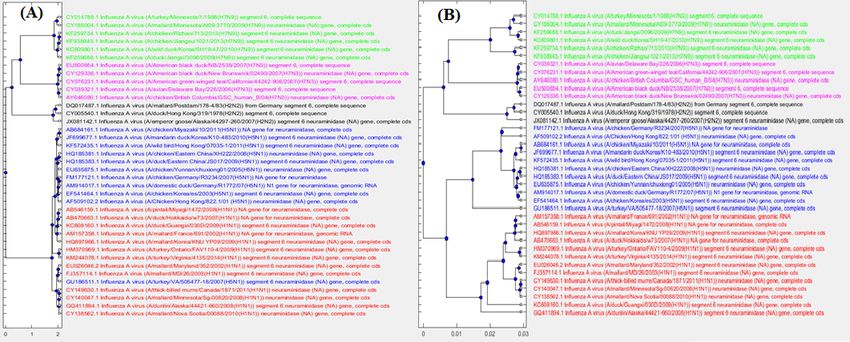
Finally Figures 6 and 7 display the phylogenetic trees generated by each of the
four methods considered. Fig 6(A), the tree generated by FFP, has many misclassi-
fied genomes, which was expected given the MoDMap visualization of its distance
matrix in Fig 5(A). Fig 7(A) displays the phylogenetic tree generated by MEGA7,
which was the same for both MUSCLE and CLUSTALW: It has only one incorrectly
classified H5N1 genome, placed in middle of H1N1 genomes. Fig 6(B) and Fig 7(B)
display the phylogenetic tree generated using the distance produced by ML-DSP
(shown twice, in parallel with the other trees, for ease of comparison). ML-DSP
classified all genomes correctly.bioRxiv preprint first posted online Aug. 20, 2018; doi: http://dx.doi.org/10.1101/394932. The copyright holder for this preprint
(which was not peer-reviewed) is the author/funder, who has granted bioRxiv a license to display the preprint in perpetuity.
It is made available under a CC-BY 4.0 International license.
Randhawa et al. Page 15 of 23
Figure 6 Phylogenetic tree comparison: FFP with ML-DSP. The phylogenetic tree
generated for 38 influenza virus genomes using (A): FFP (B): ML-DSP.
Figure 7 Phylogenetic tree comparison: MEGA7(MUSCLE/CLUSTALW) with
ML-DSP. The phylogenetic tree generated for 38 influenza virus genomes using (A):
MEGA7(MUSCLE/CLUSTALW) (B): ML-DSP.
Discussion
The computational efficiency of ML-DSP is due to the fact that it is alignment-free
(hence it does not need multiple sequence alignment), while the combination of
1D numerical representations, Discrete Fourier Transform and Pearson Correlation
Coefficient makes it extremely computationally time efficient, and thus scalable.
ML-DSP is not without limitations. We anticipate that the need for equal length
sequences and use of length normalization could introduce issues with examina-
tion of small fragments of larger genome sequences. Usually genomes vary in length
and length normalization always results in adding (up-sampling) or losing (down-
sampling) some information. Although the Pearson Correlation Coefficient can dis-
tinguish the signal patterns even in small sequence fragments, and we did not
find any considerable disadvantage while considering complete mitochondrial DNA
genomes with their inevitable length variations, length normalization may cause
issues when we deal with the fragments of genomes, and the much larger nuclear
genome sequences.
Lastly, ML-DSP has two drawbacks, inherent in any supervised machine learning
algorithm. The first is that ML-DSP is a black-box method which, while producing
a highly accurate classification prediction, does not offer a (biological) explana-bioRxiv preprint first posted online Aug. 20, 2018; doi: http://dx.doi.org/10.1101/394932. The copyright holder for this preprint
(which was not peer-reviewed) is the author/funder, who has granted bioRxiv a license to display the preprint in perpetuity.
It is made available under a CC-BY 4.0 International license.
Randhawa et al. Page 16 of 23
tion for its output. The second is that it relies on the existence of a training set
from which it draws its “knowledge”, that is, a set consisting of known genomic
sequences and their taxonomic labels. ML-DSP uses such a training set to “learn”
how to classify new sequences into one of the taxonomic classes that it was trained
on, but it is not able to assign it to a taxon that it has not been exposed to.
Conclusions
We proposed ML-DSP, an ultrafast and accurate alignment-free supervised machine
learning classification method based on digital signal processing of DNA sequences
(and its software implementation). ML-DSP successfully addresses the limitations
of alignment-free methods identified in [7], as follows:
(i) Lack of software implementation: ML-DSP is supplemented with freely available
source-code. The ML-DSP software can be used with the provided datasets
or any other custom dataset and provides the user with any or all of: pairwise
distances, 3D sequence interrelationship visualization, phylogenetic trees, or
classification accuracy scores.
(ii) Use of simulated sequences or very small real-world datasets: ML-DSP was
successfully tested on a variety of real-world datasets. We considered all
complete mitochondrial DNA sequences available on NCBI at the time of
this study. Also, we tested ML-DSP in different evolutionary scenarios such
as different levels of taxonomy (domain to genus), small dataset (38 se-
quences), large dataset (4,322 sequences), short sequences (1,136 bp), long
sequences (1,999,595 bp), benchmark datasets of influenza virus and mam-
malian mtDNA genomes etc.
(iii) Memory overhead: ML-DSP uses neither k-mers nor any compression algo-
rithms. Thus, scalability does not cause an exponential memory overhead,
and high accuracy is preserved on large datasets.
Methods
The main idea behind ML-DSP is to combine supervised machine learning tech-
niques with digital signal processing, for the purpose of DNA sequence classification.
More precisely, for a given set S = {S1 , S2 , . . . , Sn } of n DNA sequences, ML-DSP
uses:
- DNA numerical representations to obtain a set N = {N1 , N2 , . . . , Nn } where
Ni is a discrete numerical representation of the sequence Si , 1 ≤ i ≤ n.
- Discrete Fourier Transform (DFT) applied to the length-normalized digital sig-
nals Ni , to obtain the frequency distribution; the magnitude spectrum Mi of
this frequency distribution is then obtained.
- Pearson Correlation Coefficient (PCC) to compute the distance matrix of all
pairwise distances for each pair of magnitude spectra (Mi , Mj ), where 1 ≤
i, j ≤ n.
- Supervised Machine Learning classifiers which take the pairwise distance matrix
for a set of sequences, together with their respective taxonomic labels, in abioRxiv preprint first posted online Aug. 20, 2018; doi: http://dx.doi.org/10.1101/394932. The copyright holder for this preprint
(which was not peer-reviewed) is the author/funder, who has granted bioRxiv a license to display the preprint in perpetuity.
It is made available under a CC-BY 4.0 International license.
Randhawa et al. Page 17 of 23
training set, and output the taxonomic classification of a new DNA sequence.
To measure the performance of such a classifier, we use the 10-fold cross-
validation technique.
- Independently, Classical MultiDimensional Scaling (MDS) takes the distance
matrix as input and returns an (n × q) coordinate matrix, where n is the
number of points (each point represents a unique sequence from set S) and q
is the number of dimensions. The first three dimensions are used to display a
MoDMap, which is the simultaneous visualization of all points in 3D-space.
DNA numerical representations
To apply digital signal processing techniques to genomic data, genomic sequences
are first mapped into discrete numerical representations of genomic sequences, called
genomic signals [48].
In our analysis of various numerical representations for DNA sequences, we consid-
ered only 1D numerical representations, that is, those which produce a single output
numerical sequence, called also indicator sequence, for a given input DNA sequence.
We did not consider other numerical representations, such as binary [29], or nearest
dissimilar nucleotide [49], because those generate four numerical sequences for each
genomic sequence, and would thus not be scalable to classifications of thousands of
complete genomes.
Discrete Fourier Transform (DFT)
Our alignment-free classification method of DNA sequences makes use of the Dis-
crete Fourier Transform (DFT) magnitude spectrum of the discrete numerical se-
quences (discrete digital signals) that represent DNA sequences. In some sense,
these DFT magnitude spectra reflect the nucleotide distribution of the originating
DNA sequences.
To start with, assuming that all input DNA sequences have the same length p, for
each DNA sequence Si = (Si (0), Si (1), . . . , Si (p − 1)), in the input dataset, where
1 ≤ i ≤ n, Si (k) ∈ A, C, G, T , 0 ≤ k ≤ p − 1, we calculate its corresponding
discrete numerical representation (discrete digital signal) Ni defined as
Ni = (f (Si (0)), f (Si (1)), . . . , f (Si (p − 1)))
where, for each 0 ≤ k ≤ p−1, the quantity f (Si (k)) is the value under the numerical
representation f of the nucleotide in the position k of the DNA sequence Si .
Then, the DFT of the signal Ni is computed as the vector Fi where, for 0 ≤ k ≤
p − 1 we have
p−1
X
Fi (k) = f (Si (j)) · e(−2πi/p)kj (1)
j=0
The magnitude vector corresponding to the signal Ni can now be defined as
the vector Mi where, for each 0 ≤ k ≤ p − 1, the value Mi (k) is the absolutebioRxiv preprint first posted online Aug. 20, 2018; doi: http://dx.doi.org/10.1101/394932. The copyright holder for this preprint
(which was not peer-reviewed) is the author/funder, who has granted bioRxiv a license to display the preprint in perpetuity.
It is made available under a CC-BY 4.0 International license.
Randhawa et al. Page 18 of 23
value of Fi (k), that is, Mi (k) = |Fi (k)|. The magnitude vector Mi is also called the
magnitude spectrum of the digital signal Ni and, by extension, of the DNA sequence
Si . For example, if the numerical representation f is Integer (row 1 in Table 2),
then for the sequence S1 = CGAT , the corresponding numerical representation is
N1 = (1, 3, 2, 0), the result of applying DFT is F1 = (6, −1 − 3i, 0, −1 + 3i) and
its magnitude spectrum is M1 = (6, 3.1623 , 0, 3.1623).
Fig 8A shows the discrete digital signal (using the PP numerical representa-
tion, row 6 of Table 2) of the DNA sequence consisting of the first 100 bp of
the mtDNA genome of Branta canadensis (Canada goose, NCBI accession number
N C 007011.1), and of the DNA sequence consisting of the first 100 bp of the mtDNA
genome of Castor fiber (European beaver; NCBI accession number N C 028625.1).
Fig 8B shows the DFT magnitude spectra of the same two signals/sequences. As
can be seen in Fig 8B, these mtDNA sequences exhibit different DFT magnitude
spectrum patterns, and this can be used to distinguish them computationally by
using. e.g., the Pearson correlation coefficient, as described in the next subsection.
Other techniques have also been used for genome similarity analysis, for example
comparing the phase spectra of the DFT of digital signals of full mtDNA genomes,
as seen in Figure 9 and [50, 51].
Note that, with the exception of the example in Fig 8, all of the computational
experiments in this paper use full genomes.
Figure 8 Canada goose (blue) vs European beaver (red): comparison of the DFT
magnitude spectra of the first 100 bp of their mtDNA genomes. (A): Graphical
illustration of the discrete digital signals of the respective DNA sequences, obtained using the PP
representation. (B): DFT magnitude spectra of the signals in (A).You can also read