MmWave Radar for Automotive and Industrial Applications - December 7, 2017 Karthik Ramasubramanian - Texas Instruments
←
→
Page content transcription
If your browser does not render page correctly, please read the page content below
mmWave Radar for Automotive and
Industrial Applications
December 7, 2017

Karthik Ramasubramanian
Distinguished Member of Technical Staff, Texas Instruments

                                                             1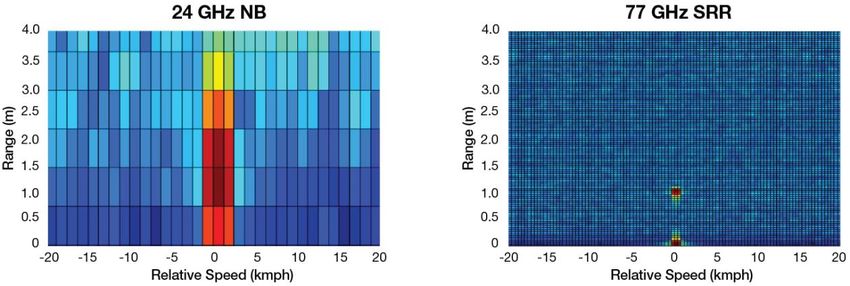
Introduction
• Radar technology has been in existence for several decades
                                                                     LRR/MRR
   – Military, Weather, Law enforcement, and so on
• In the past decade, use of radar has exponentially increased
   – Automotive and Industrial applications
• Automotive applications
   – Front-facing radar (LRR/MRR)
      • Adaptive Cruise Control, Autonomous Emergency Braking
   – Corner radar (SRR)
      • Blind Spot Detection, Lane Change Assist, Front/Rear Cross
        Traffic Alert
   – Newer applications                                                  SRR

      • Automated parking, 360 degree surround protection
      • Body/Chassis and In-cabin applications
• Industrial applications
   –   Fluid level sensing
   –   Solid volume identification
   –   Traffic monitoring and Infrastructure systems
   –   Robotics, and many others                                          2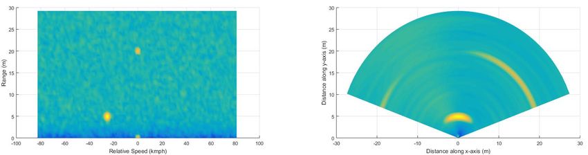
77GHz mmWave Radar
• mmWave: RF frequencies within 30 GHz to 300 GHz
  – Wavelength is in the order of few millimeters
• 77GHz mmWave radar bands
  – 76-77 GHz
     • Allocated for vehicular radar in many countries
     • Also available for infrastructure systems in certain regions
  – 77-81 GHz
     • Recently made available for short range radar
     • Legacy 24 GHz UWB short range radar to be phased out by 2022
  – 75-85 GHz: Available for level probing radar
• mmWave radar sensors can measure
  – Radial distance (range) to the object
  – Relative radial velocity to the object
  – Angle of arrival using multiple TX, RX
• Some benefits of radar
  – Robust to environmental conditions like dust/fog/smoke
  – Operation in dazzling light, or no ambient light
  – Operation behind plastic enclosure                                3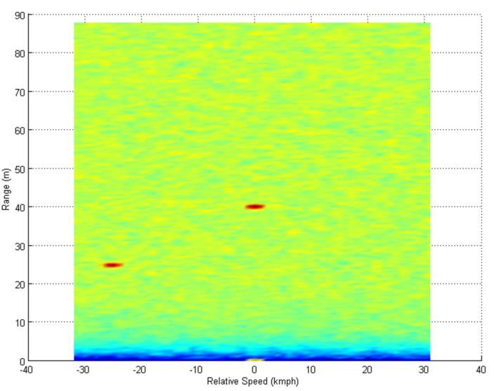
FMCW Radar – Overview
• Multiple types of radar modulation
waveforms used FMCW – Freq vs. Time sawtooth pattern
– Pulsed radar, CW Doppler radar, UWB,
2R
FSK, FMCW, PN-modulated radar fTx(t) td
c
• FMCW: Frequency Modulated fRx(t) B (in 100’s of
Continuous Wave MHz or few
GHz)
– FMCW (sometimes called LFMCW or fIF
Linear FMCW) is the most commonly (few MHz)
used scheme in automotive radar today t
Tchirp
– Linear FMCW: TX signal has frequency
changing linearly with time (i.e., chirp)
• Key benefits of FMCW radar
– Ability to sweep wide RF bandwidth (GHz) while keeping IF bandwidth small (MHz)
• Better range resolution. RF sweep bandwidth of 2 GHz can achieve 7.5cm range resolution,
while IF bandwidth can still be
FMCW Radar – System Model (1/3) 1. TX signal
• High-level block diagram
Ramp
waveform
gen.
• The transmitted FMCW waveform (chirp) is
B
xT (t ) cos 2f c t t 2
Tc
T(t) Tc
B Sweep bandwidth of transmitted chirp (Hz)
fT(t)
Tc Chirp duration (s)
• The instantaneous frequency of FMCW B
waveform is 1 dT (t )
fT (t )
2dt fc
B
fc t t
Tc Tc 5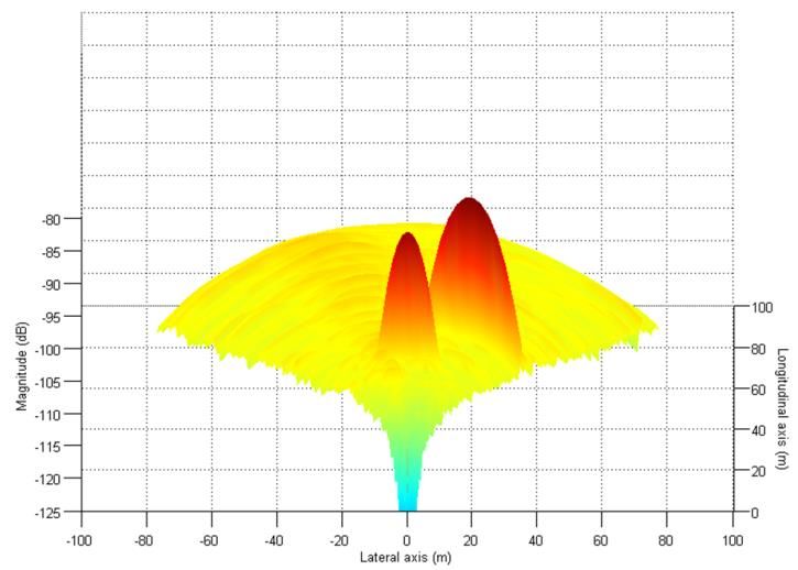
FMCW Radar – System Model (2/3) 2. RX signal
• High-level block diagram
Ramp
R waveform
gen.
R
• Received signal is a scaled and delayed version of transmitted signal
B
xR (t ) xT (t t d ) cos 2f c (t t d ) (t t d ) 2 td
2R
Tc c
Path loss attenuation
t d Time delay of reflection (from object) fT(t)
fR(t)
• Round-trip delay of reflection td is
2R fIF(t)
td
c
R Range (Distance) of the object t
c Speed of light Tc 6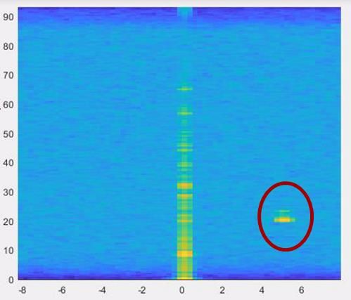
FMCW Radar – System Model (3/3) 3. Beat signal
• High-level block diagram (IF)
Ramp
R waveform
gen.
R
IF signal
• Beat frequency or IF signal after receive mixer is as follows
y (t ) xR (t ) xT (t ) cosT (t t d ) cosT (t ) 2R
td
c
y (t ) cosT (t td ) T (t ) cosT (t td ) T (t )
2
Can be calculated as Filtered out in the fT(t)
receiver
B
0 2 t d t fR(t)
c
T
fIF(t)
Beat frequency t
corresponding to the target Tc 7
FMCW Radar – How it works (1/2) Static objects
• For static objects, the beat frequency is simply
proportional to the distance (round-trip delay)
• Beat frequency is the product of FMCW
frequency slope (B/Tc) and round-trip delay (td)
• For multiple objects, the beat signal is a sum of
tones, where each tone’s frequency is
proportional to the distance of the object
• The frequencies of these tones gives the
distances to the different objects
• Detection of objects and Distance (Range)
estimation is done typically by taking FFT of
received IF signal
Beat freq = Round-trip delay * Slope
2 R B
fb
c Tc 8
FMCW Radar – How it works (2/2) Moving objects
• For moving objects, velocity (v) is determined using phase change across
multiple chirps
• Phase and frequency of the received beat signal for the nth chirp can be
calculated as
New terms in beat frequency
2v 2v B
0 2 f c n Tc 2 ( f c n B ) t d t
c c Tc
Phase change from chirp-to-chirp
that depends only on the velocity
(not on range)
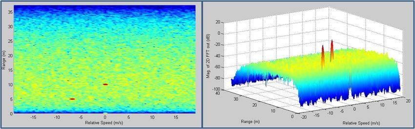
• Second dimensional FFT is performed across chirps to determine the phase
change and thus the velocity
• The two-dimensional FFT process gives a
2D range-velocity image (FFT heatmap)
• Typically, detection of objects is done on
this image
• After detection, the range and relative
speed of the objects are easily calculated
9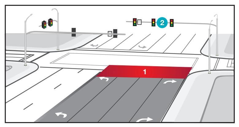
Angle Estimation - Beamforming

    θ
                    Δ=dsin(θ)
            θ

        A   d      Aejw           Aej2w        Aej3w
                  Uniform linear array

• Consider received signal for multiple RX antennas (say, four) as shown in figure
• Additional distance (Δ) travelled at successive antennas depends on the angle of
  arrival θ

• This additional distance results in a phase change (w) across consecutive antennas

• This phase change can be estimated (west) using an FFT (3rd dimension FFT)
• Once w is estimated, the angle of arrival (θ) can be derived easily
Sample FMCW Radar processing flow (1/2)
• Typical processing flow used in FMCW (sawtooth) Radar signal processing
Pre- Log-Mag &
ADC processing 1st dim FFT 2nd dim FFT Detection
(Range FFT) (Doppler FFT)
output (DC removal, Interf (CFAR-CA /
CFAR-OS) Raw point Tracked
mitigation)
cloud objects
Angle Clustering,
Estimation Tracking
(Higher layer
(3rd dim FFT)
algorithms)
2D FFT heatmap
Longitudinal axis (m)
Range (m)
Relative Radial Velocity Lateral axis (m) 11Sample FMCW Radar processing flow (2/2)
• Typical (simple) FMCW chirp configuration consists of a sequence of chirps followed by idle time
Frame time (~40ms)
Active transmission time of chirps
(10~15 ms) Inter-frame time
(upto 25~30ms)
time
1D FFT processing is done inline. 2D-FFT, 3D-FFT & Detection for current frame.
CFAR or other proprietary algorithms often used for detection.
A frame consists of active transmission
time and idle inter-frame time.
First-dimension FFT
(Range FFT)
Rx1,2,3,4
Second-dimension FFT
(Doppler FFT)
Radar data cube memoryAdvantages of Fast FMCW modulation
• Slow FMCW (Triangular)
waveform used in many Slow (Triangular) FMCW
legacy systems
– Chirp duration in ms,
instead of us
• Slow FMCW has
advantage of low DSP
MIPS requirement
– No two-dimensional FFT
processing
• However, it suffers from
ambiguity issues
– No elegant way of getting Fast (sawtooth) FMCW
range-doppler image
• Fast FMCW (Sawtooth)
waveform is preferred in
newer systems
• Fast FMCW has ability to
provide range-doppler
two dimensional image of
objects 13Radar system performance parameters
• Key parameters
– Max range
– Range resolution
– Range accuracy Rmax
Rmax
– Max velocity
– Velocity resolution R R
R
– Velocity accuracy R
– Field of view V
v
– Angular resolution
– Angular accuracy
– Cycle time
VmaxRx signal level
Max range (1/2)
Pt Gt (RCS) Gr 2 Tf
SNR =
• Based on Friis transmission equation (linear scale)
(4R2) (4R2) 4 (kT)(NF)
Noise level
Pt 12dBm
1/(4R2)
TX Gt 12 dBi
Radar device
80m
RCS
RX Gr 12 dBi 1/(4R2) 1m2
2
4
RX signal level:
Noise level: -174 dBm/Hz + 16 dB + 10*log10(100 Hz) = -138dBm
= -121 dBm
Thermal noise Noise figure 10ms active frame (Tf)
floor (kT) (NF) (integration time) SNR = 17dBMax range (2/2) Pt Gt (RCS) Gr2 Tf
Rmax =
4 (4)3 (SNR) (kT)(NF)
• Max range depends on the below factors
Typical range
Azim Elev
TX Output power 10 dBm – 13 dBm FOV FOV Antenna
(deg) (deg) gain (dB)
TX Antenna gain 9 dBi – 23 dBi Depends on Azimuth and SRR 120 30 9.21
(USRR – LRR) Elevation field of view MRR 90 12 14.44
RCS of target 0.1m2 – 50m2 Pedestrian vs. Truck LRR 24 8 21.94
(-10 dBsm to 17 dBsm)
Target RCS
RX Antenna gain 9 dBi – 23 dBi Depends on Azimuth and Pedestrian 0.1 ~ 1 sq.m
Elevation field of view
Motorbike 5 sq.m
Noise figure 11 dB – 18 dB Car 10 sq.m
Implementation dependent Truck 50 sq.m
Active frame time 2 ms – 20 ms
Thumb rule:
Detection SNR 10 dB – 18 dB 3 dB loss = 15% loss of range
12 dB loss = 50% loss of range
RX array beamforming gain can be additionally included.Range resolution and Range accuracy
1
• Range resolution H( f )
f
Tc
– Ability to separate two closely spaced objects in
range 3dB
– Range resolution is a function of RF bandwidth
used
2 R B
fb
f
c Tc 2 R B
fb
c Tc
2R B 2( R R ) B
f f b f
c Tc c Tc
Sweep BW Range resolution
1 c
But f , therefore, R (MHz) (cm)
Tc 2B 200 75
600 25
1000 15
• Range accuracy 2000 7.5
– Accuracy of range measurement of one object 4000 3.75
– Depends on SNR
– Typically range accuracy is a small fraction of
range resolution c
R
3.6 B 2 SNRMax velocity
• Max unambiguous velocity in Fast
FMCW modulation depends on chirp
repetition period Total Chirp Max unamb velocity
– Higher velocity needs faster ramps
duration (us) (+/-kmph)
50 70
= wavelength 38 92
vmax Tc = Total chirp duration
4Tc (incl. inter-chirp time)
25 140
• For a given max range and range
resolution, higher max velocity needs
higher IF bandwidth
Max
range
IF
bandwidth
Max
Range
unamb.
resolution
velocity
• Advanced techniques are often used
to increase the max velocity
– Ambiguity resolution techniques can be
used to resolve aliased velocity into
true velocityVelocity resolution and Velocity accuracy
• Velocity resolution Active Frame Velocity resolution
– Ability to separate two objects in velocity duration (ms) (+/-kmph)
– Depends on the active duration of the frame 5 1.40
10 0.70
= wavelength
v N = number of chirps in the frame
15 0.47
2 NTc Tc = Total chirp duration 20 0.35
(incl. inter-chirp time)
• Velocity accuracy
– Accuracy of velocity measurement of one object
– Depends on SNR
– Typically a fraction of velocity resolution
v
3.6 NTc SNRBenefits of 77GHz mmWave
• Wide RF bandwidth (4 GHz) provides good range resolution and range accuracy
– 20X better than legacy 24GHz narrowband sensors (which use ~200MHz bandwidth)
• High RF frequency (small wavelength) provides good velocity resolution and accuracy
– 3X better than 24GHz sensors
Improved performance
Better resolution performance with 77GHz
More focused beam with 77GHz
• Smaller form-factor for the sensor
20Angular resolution
• Angular resolution
– Ability to separate objects in angle (for same range
and velocity)
– Radar sensors have poorer angular resolution
typically (compared to LIDAR for example)
– However, in many real life situations, objects get
resolved in range or velocity, due to good resolution
in those dimensions
– Angular resolution (in radians) for K-length array is
given by:
Ang. Resolution
Array length (deg)
λ
= Kdcos(θ) Note the dependency of the resolution on θ. 8 14.32
(in radians)
Resolution is best at θ=0 12 9.55
24 4.77
2
= K Resolution is often quoted assuming d=λ/2 and θ=0 40 2.86Use of Multiple TX – MIMO radar
• Multiple TX along with multiple RX (MIMO radar) to increase angular resolution – eg. 2 TX, 4 RX can give 8
virtual channels
Tx1 Tx2 Rx1 Rx4 8 virtual channels
2 /2 /2
Multiple TX time-interleaved Frame time (~40ms)
Active transmission time of chirps
(Tx1 and Tx2 chirps interleaved) Inter-frame time
Tx1 Tx2 Tx1 Tx2 Tx2
time
Multiple TX BPM-multiplexed
Frame time (~40ms)
Active transmission time of chirps
(Tx1 and Tx2 BPM-coded, simultaneous transmission)
Inter-frame time
Tx1+Tx2 Tx1-Tx2 Tx1+Tx2
time
• Multiple TX can also be used for TX beamsteering (simultaneous transmission with linear phase shifter
based steering of beam)Cascaded multi-chip radar
RX TX RX TX Measurement results with 2 corner reflectors at ~4deg separation
8 channels (2 TX, 4 RX) 12 channels (3 TX, 4 RX)
Single chip Single chip
Slave device Master device 24 channels (3 TX, 8 RX) 40 channels (5 TX, 8 RX)
(LO sync’ed to master)
2-chip cascade 2-chip cascade
Two corner reflectors 2-chip cascade radar 2-chip cascade enables better separation of the corner reflectors
23TI mmWave radar devices
• TI offers a family of 77GHz radar devices for automotive and industrial applications
– Highly integrated devices based on RFCMOS
– High accuracy, Small form-factor, Sensing simplified
For more information, visit:
TI.com/mmWaveReferences
• M. Skolnik, Introduction to Radar Systems, McGraw-Hill, 1981
• Donald E. Barrick, “FM/CW Radar Signals and Digital Processing”, NOAA Technical Report
ERL 283-WPL 26, July 1973
• A. G. Stove, ‘‘Linear FMCW radar techniques’’, IEE Proceedings F, Radar and Signal
Processing, vol. 139, pp. 343-350, October 1992
• M. Schneider, ‘‘Automotive Radar Status and Trends’’, in German Microwave Conference
(GeMiC), pp. 144-147, Ulm, Germany, April 2005
• TI whitepapers
– The fundamentals of millimeter wave – Available at http://www.ti.com/lit/spyy005
– Highly integrated 77GHz FMCW Radar front-end: Key features for emerging ADAS applications –
Available at http://www.ti.com/lit/spyy003
– TI’s smart sensors enable automated driving – Available at http://www.ti.com/lit/spyy009
– AWR1642: Radar-on-a-chip for short range radar applications – Available at http://www.ti.com/lit/spyy006
– Fluid-level sensing using 77 GHz millimeter wave – Available at http://www.ti.com/lit/spyy004
– Robust traffic and intersection monitoring using millimeter wave radar – Available at
http://www.ti.com/lit/spyy002
25You can also read