Modelling the Economy-Wide Marginal Impacts Due to Climate Change in Australian Agriculture
←
→
Page content transcription
If your browser does not render page correctly, please read the page content below

Modelling the Economy-Wide Marginal Impacts Due to
 Climate Change in Australian Agriculture

 CoPS Working Paper No. G-312, February 2021

 Glyn Wittwer
 Centre of Policy Studies,
 Victoria University

ISSN 1 921654 02 3 ISBN 978-1-921654-20-6

 The Centre of Policy Studies (CoPS), incorporating the IMPACT project, is a research centre at Victoria
 University devoted to quantitative analysis of issues relevant to economic policy.
 Address: Centre of Policy Studies, Victoria University, PO Box 14428, Melbourne, Victoria, 8001
 home page: www.vu.edu.au/CoPS/ email: copsinfo@vu.edu.au Telephone +61 3 9919 1877
About us
Researchers at the Centre of Policy Studies have a 45-year history of
continuous achievement in the development, application and
dissemination of large-scale economic models. Our models and software
are used around the world to analyse a diverse range of economic
issues. CoPS’ funders include: Australian federal and state government
departments; private firms and universities in many parts of the world;
central government agencies such as finance and trade ministries in
many countries; and international development organisations. The
Centre’s GEMPACK software, used for solving large economic models,
is used at more than 700 sites in over 95 countries.

Citation
Wittwer, Glyn (2021), “Modelling the economy-wide marginal
impacts due to climate change in Australian agriculture”, Centre of
Policy Studies Working Paper No. G-312, Victoria University,
February 2021.
1

 Modelling the economy-wide marginal impacts due to climate change in
 Australian agriculture
 Author: Glyn Wittwer

 Abstract
 The decade from 2011 to 2020 started with the tail end of one of the wettest two
 year periods observed in eastern Australia and ended with recovery from the
 hottest and driest year ever recorded. An increasing prevalence of extremes is
 consistent with expectations concerning climate change.
 This study uses observed rainfall and temperature anomalies to infer farm
 productivity levels by region. Productivity shocks are run year-by-year in the multi-
 regional VU-TERM model. The three scenarios of the study include a decade
 reflecting 2011 to 2020 seasons, a “2030” scenario in which farm productivity falls
 by 10% relative to the first scenario in five of the 10 seasons and a “2050”
 scenario in which, in the corresponding years, farm productivity falls 20%.
 The welfare impact of the first scenario relative to a baseline without year-on-year
 seasonal variations is minus $35 billion in net present value terms. The welfare
 impact in the second scenario is minus $46 billion and minus $59 billion in the
 third scenario.
 Welfare losses are alleviated to a small extent by resource movements. In
 particular, in years in which drought induces collapses in productivity, livestock
 production switches from grazing to fodder inputs. The study assumes that
 Outback Queensland consists of rangeland production in which a switch to fodder
 is not feasible. The region’s income losses in drought are worse than elsewhere.
 Lack of input flexibility contributes to the region’s losses.

 JEL classification: C68; Q54; R11; R15
 Keywords: regional drought impacts; climate change; welfare; adaptation
2
3

Contents

 1. Introduction 4
 2. VU-TERM modelling 4
 3. The first scenario – a “2020” decade 5
 4. The “2030” and “2050” scenarios 10
 5. Industry composition changes 12
 6. Welfare impacts 13
 7. Conclusion and research possibilities 14
References 14
Appendix A: maps of historical rainfall and temperature variation and
accompanying agricultural productivity levels 16
Appendix B: General information on VU-TERM 27
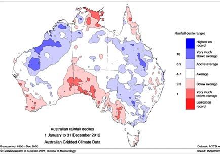
4

Modelling the economy-wide marginal impacts due to climate change in Australian
agriculture
 1. Introduction
Evidence is mounting of climate change within Australia. The Bureau of Meteorology reports
that the mean temperature nationally in the decade ending 2020 was 0.95C above average,
and 0.33C above the previous decade. Since 2013, every year has been among the ten
warmest ever recorded. 1 In the southwestern part of Western Australia, annual rainfall has
declined by up to 20% since the early 1970s. This has resulted in streamflow declines of
around 80%. The year 2019 was the hottest and driest ever recorded. Australia received
global attention when bushfires razed 5.6 million hectares across the nation in the summer of
2019-20. Most of the fires occurred in relatively high rainfall areas along the Great Dividing
Range and towards the coast in southeastern Australia. Unprecedented low soil moisture
conditions resulted in unprecedented vulnerability to bushfires. 2
The objective of this study is to concentrate on one dimension of climate change. The study is
confined to regional impacts of climate on agricultural output using a dynamic, multi-
regional CGE model.
 2. VU-TERM modelling
VU-TERM is the CGE model used in this study. There are three climate scenarios. Actual
mean rainfall and temperature recorded from 2016 to 2020, and from 2011 to 2015, provide
the basis for the first run. Year 1 agricultural productivity reflects 2016 conditions, year 2
2017 conditions and so to year 5. Thereafter, year 6 reflects 2011 conditions, up to year 10
reflecting 2015 conditions (see appendix A).
The baseline against which we compare the deviations in model runs is relatively bland,
consisting of “average” seasons with baseline productivity. Farmers prefer relatively
“average” conditions but there is a tendency with climate change for extremes to occur more
frequently. The decade ending 2019 provides a stark example, with the two-year period of
2010-2011 being among the wettest ever recorded over substantial parts of eastern Australia
and 2018-2019 being the driest recorded over much of the southeastern quadrant of the
continent. But even in the relatively high rainfall event of 2010-2011, when we might expect
temperatures to be lower, temperatures were near the long-term average. In the 2018-2019
drought, mean temperatures were more than 1.5C degrees above the mean over most of the
southeastern quadrant.
We can think of the first run as a stylized version of 2020 climatic conditions. In a second
run, a stylized depiction of 2030, the years of drought have the same farm productivity levels
as those of the first run. In the “2030” set, productivity levels are 10% worse than the first run
in years 1, 5, 7, 9 and 10. Finally, in the “2050” set of runs, productivity levels in the same
five years are 20% worse than in the first run, while keeping productivity levels the same as
the first run in years 2, 3, 4, 6 and 8.
The productivity assumptions for the “2030” and “2050” runs may underestimate impacts due
to rising temperatures. The objective of this study is not to work with the “most likely”

1
 See http://www.bom.gov.au/climate/current/annual/aus/
2
 See http://www.bom.gov.au/water/landscape/#/sm/Relative/day/-28.37/130.43/4/Point////2019/12/31/
5

scenario, but rather to provide a framework to quantify the economic impacts and responses
to climate change. Refined runs may follow in future studies.
The advantages of this approach is that it includes greater regional detail and greater year-by-
year texture than past CGE modelling efforts. Each of these matters. Inland farming regions
appear to be more vulnerable than coastal regions to rising temperatures. 3 The biggest
impacts from climate change do not arise from changes in rainfall and temperatures averages,
but from extremes. To illustrate, in 2019, the driest and hottest year ever in Australia, a flood
hit Townsville and regions to west in late January, dumping 1400mm of rain on Townsville
in around 10 days. This resulted in both a short-lived cessation of economic activity in the
city plus longer term impacts on damaged housing, crops and infrastructure, none of which is
modelled in this study. It was an extreme flood event in a time of drought.
Many previous modelling efforts have used adaptations of the multi-country, global GTAP
model (Liu et al. (2016) is one example). GTAP has one important advantage over TERM-
VU: it can estimate terms-of-trade impacts arising from changes in relative global scarcity.
This implies that it is possible for a particular nation to suffer a decrease in farm output, yet
more than offset that decrease via a terms-of-trade gain arising from global price increases for
farm outputs. The VU-TERM results presented in this study assume that there is no ongoing
outward export demand shifts for farm produce arising from worsening global relative
scarcity.
Future studies may include modifications to GTAP variants or add biophysical accounts to
VU-TERM for variables including soil moisture, groundwater levels and river flows. Studies
using VU-TERM may include more detailed inputs concerning climate variation, and also
use modelled relative price impacts from GTAP as exogenous export demand or import
supply shifts.
 3. The first scenario – a “2020” decade
The first scenario models two phases in the “2020” decade. First, years 1 to 5 (i.e, 2016 to
2020) use observed regional annual rainfall and temperature differences from average to infer
farm productivity levels for each region. An appendix shows the rainfall and temperatures
and the farm productivity levels for each year based on these. Year 6 to 10 are based on
historical annual rainfall and temperature differences for 2011 to 2015.
In years of drought, productivity falls sharply relative to base in agricultural sectors in farm-
affected regions.
GDP on the income side is a function of primary factors (capital K and employment L) and
underlying technology (1/A):
 1
 = ( , , ) (1)

Although agriculture accounts for little more than 2% of GDP, wide variations in seasonal
conditions can make significant contributions to national income fluctuations. This is evident
in figure 1, in which real GDP falls to 1% below base in year 4, which reflects the historical

3
 An exception is in tropical region, in which new agricultural developments tend to be away from the coast, due
to expectation of more severe cyclones in the future.
6

seasonal inputs to 2019-20 (i.e., 2019, the hottest and driest year on record in Australia).
Some of the decline in capital, which falls to as much as 0.2% below base, arises from culled
livestock in drought years, and some from depressed investment in drought years (figure 2).
Figure 1: Real GDP, national, income side; labour market

(% deviation from base)

Drought-induced productivity losses weaken the labour market. Figure 1 shows that within
the theory of the model, productivity losses depress both real wages and employment relative
to base. 4 In year 5, which is a recovery year, aggregate investment rises above base, and
employment rises with it (figures 1 and 2).
Figure 2: National aggregate consumption and investment
(% deviation from base)

4
 Prior to COVID-19, wages growth had been slow for a number of years. Drought contributed to diminishing
real wages growth.
7

Figure 3: Income-side real GDP at the Northern and Central Victoria
regional level, “2020” scenario
(% deviation from base)
Capital Region, NSW

 Darling Downs-Maranoa-Granite Belt, Qld

Central West, NSW

Far West – Orana, NSW Outback Queensland

Riverina—Murray NSW Eyre Peninsula, Mallee and Outback, SA

New England – North West – Grafton Wheatbelt, WA
8

Figure 4: Income-side real GDP at the Northern and Central Victoria
regional level, “2030” scenario
(% deviation from base)
Capital Region, NSW

 Darling Downs-Maranoa-Granite Belt, Qld

Central West, NSW

 Outback Queensland

Far West – Orana, NSW

 Eyre Peninsula, Mallee and Outback, SA
Riverina—Murray NSW

 Wheatbelt, WA
New England – North West – Grafton
9

Figure 5: Income-side real GDP at the Northern and Central Victoria
regional level, “2050” scenario
(% deviation from base)
Capital Region, NSW

 Darling Downs-Maranoa-Granite Belt, Qld

Central West, NSW

 Outback Queensland

Far West – Orana, NSW

 Eyre Peninsula, Mallee and Outback, SA
Riverina—Murray NSW

New England – North West – Grafton Wheatbelt, WA
10

The impacts in relatively agriculture-intensive regions are proportionally much greater than
those at the national level. Figure A2 shows agriculture’s share of GDP for each in the model.
In Far West-Orana, New England-North West-Grafton, Darling Downs-Maranoa-Granite
Belt and Outback Queensland, there are prolonged periods in which real GDP falls more than
8% below base in the “2020” scenario. In figure 1 and figures 3 to 5, drought-induced
technological deterioration is evident. Real GDP is a macro measure of output. In years 3 and
4, the percentage fall in real GDP is larger than the percentage fall in labour or utilized capital
at the national level and in many of the regions shown. From equation (1), technological
deterioration explains the gap between the percentage deviation in factor inputs and real
GDP. In any drought-affected region, real GDP will fall further than the share-weighted sum
of primary factors.
Employment nationally falls to more than 0.7% or more than 70,000 jobs below base in year
4. By assumption, real wages adjust sluggishly at the regional level. In circumstances of
severe regional downturns, we expect real wages adjustment to be limited: any workers who
are relatively mobile and even some who in normal circumstances are less mobile may leave
a region. In addition, participation rates may fall temporarily in drought. To avoid unrealistic
downward wages adjustment, exogenous temporary downward labour supply shifts are
imposed in a number of regions in year 4. Consequently, in the “2020” run, no regional real
wages fall more than 2% below base in any year. In Far West-Orana and New England-North
West –Grafton, employment is around 4% below base in year 4, reflecting an exogenous
downward labour supply shift in addition to the endogenous impacts of prolonged drought.
 4. The “2030” and “2050” scenarios
The assumption underlying the “2030” scenario is that relatively normal years are hotter and
therefore effective rainfall is less than in corresponding years of the “2020” scenario. The
“2050” scenario takes this a step further, with larger productivity declines, reflecting higher
temperatures and lower effective rainfall.
The two scenarios depict weaker recovery years and larger income losses than the “2020”
scenario in years 1, 5, 7, 9 and 10.
Figure 4 shows the regional income-side GDP impacts for the “2030” scenario and figure 5
the corresponding “2050” impacts. Among the impacts, employment is slightly lower in the
“2030” and “2050” scenarios than the “2020” scenario. If the downward labour supply shifts
were applied to later years in some regions in the “2050” scenario, employment impacts
would be larger. For example, in Outback Queensland, in which years 9 and 10 turn from
moderate drought in the “2020” scenario to severe drought in the “2050” run, a labour supply
shift would lessen the real wage drop and worsen the employment outcome, which is 1.3%
below base in year 10 (figure 7). The theory of the model allows for an endogenous decrease
in labour supply over time: it falls to 0.6% below base in year 10, not sufficient to prevent
real wages from dropping more than 2% below base in Outback Queensland in that year.
11

Figure 6: Labour markets, “2020” Northern and Central Victoria
scenario
(% deviation from base)
Capital Region, NSW

 Darling Downs-Maranoa-Granite Belt, Qld

Central West, NSW

 Outback Queensland

Far West – Orana, NSW

 Eyre Peninsula, Mallee and Outback, SA

Riverina—Murray NSW

 Wheatbelt, WA
New England – North West – Grafton
12

Figure 7: Labour market, Outback Queensland, “2050” scenario

 5. Industry composition changes
In regions other than Outback Queensland, as productivity falls due to drought, there is a
switch from pasture grazing to fodder inputs. The theory of VU-TERM includes
substitutability between land and fodder (HayCerealFod) in livestock production. A key
assumption is that fodder produced in one year may be used in another, thereby providing a
means of managing seasonal risk. We usually assume that intermediate inputs are used in the
same period as they are produced. HayCerealFod productivity shocks are not imposed in the
“2020” run, to reflect that fodder produced in good years may be used in drought years. In
rangeland production in Outback Queensland, we assume that this is not possible and that
output (i.e., herd numbers) must diminish during prolonged dry spells.
In VU-TERM, in the drought years 2 to 4, beef cattle output in New England – North West –
Grafton rises relative to base (table 1). This reflects the assumption that fodder (including
feedlotting) inputs substitute for land inputs throughout the region. 5 Beef cattle output
collapses in Outback Queensland due to an inability, by assumption, to switch to fodder in
the region. 6 The modelled outcome therefore is that even though land productivity in beef
cattle production collapses in New England – North West – Grafton, there is an increase in
output. This reflects a switch from Outback Queensland to the northern NSW region in
production, due toa relative gain in cost competitiveness in the NSW region. A lower degree
of substitutability between fodder and land in the region would lessen the switch.
In the “2030” and “2050” scenarios, in which productivity losses worsen in Outback
Queensland, the switch in output to the NSW region enlarges. This switch is not specific to
New England – North West – Grafton: it applies to all beef cattle producing regions other
than Outback Queensland. By assumption, each of these has substitutability between land and
fodder inputs in livestock production.

5
 . During the 2017-2019 drought, herd numbers across NSW declined, reflecting severe drought. The share of
cattle in feed-lotting rose in response to drought. Some farmers particularly on the Liverpool Plains, which
historically is not prone to drought, did not have fodder on hand. They faced prohibitive input costs if they
sought to maintain herd numbers.
6
 To mimic lack of substitutability, a total factor productivity shock was applied to livestock in the Queensland
Outback region instead of a land productivity shock.
13

Table 1: Farm outputs
(% deviation from base)

 Year 1

 Year 2

 Year 3

 Year 4

 Year 5

 Year 6

 Year 7

 Year 8

 Year 9

 Year
 10
 “2020”
 OthBrdAcrCrp 6.2 -9.6 -21.0 -38.5 -0.9 -0.5 -7.2 -5.2 -13.2 -10.3
 Horticulture -0.8 -3.7 -7.4 -15.0 -1.0 -3.1 -4.4 0.2 -5.3 -5.6
 Sheep 0.4 -0.4 -2.7 -3.8 -0.5 0.0 0.0 -1.4 -1.6 -1.0
 BeefCattle 0.1 -0.3 -3.5 -3.8 -0.3 0.2 0.2 -2.8 -2.1 -1.9
 Wheat 17.8 -15.2 -40.0 -48.1 -8.6 0.4 -23.8 -9.9 -21.2 -18.9
 Cotton 0.9 -10.8 -35.4 -39.3 -2.5 1.5 -2.1 -17.4 -19.1 -8.4
 HayCerealFod 0.5 -0.6 -1.4 -2.3 -0.3 -0.3 -1.0 0.0 -0.8 -0.5
 DairyCattle 0.2 -0.4 -1.5 -3.3 -1.1 -1.0 -1.2 -0.9 -1.7 -1.6
 OthLivstock 0.3 -0.4 -1.7 -2.4 -0.2 0.1 -0.1 -1.1 -1.3 -1.0
 BeefCattle (regional):
 OutbackQld 9.5 -9.9 -53.9 -55.0 -14.6 4.1 4.6 -55.0 -45.3 -45.8
 NewEngNWGrft -1.5 2.0 6.4 4.2 1.8 0.1 0.0 7.7 6.6 7.7
 “2030”
 OthBrdAcrCrp -1.7 -9.4 -20.9 -38.4 -8.0 -0.6 -14.0 -5.2 -19.9 -16.8
 Horticulture -10.7 -4.7 -8.4 -16.0 -10.1 -3.9 -13.5 -0.6 -14.3 -14.5
 Sheep -7.4 -0.8 -3.1 -4.1 -1.8 -0.4 -1.4 -1.7 -3.0 -2.4
 BeefCattle -2.8 -0.4 -3.5 -3.8 -1.1 0.1 -0.5 -3.0 -3.2 -2.9
 Wheat 6.5 -15.2 -40.1 -48.1 -16.9 0.5 -30.5 -9.8 -28.3 -25.9
 Cotton -4.5 -10.8 -35.4 -39.4 -6.6 1.4 -5.9 -17.4 -24.3 -13.0
 HayCerealFod -3.5 -0.1 -0.9 -2.0 -4.8 0.3 -5.0 0.7 -4.8 -4.2
 DairyCattle 0.1 -0.7 -1.8 -3.5 -2.1 -1.5 -2.4 -1.5 -3.1 -3.0
 OthLivstock -1.5 -0.4 -1.7 -2.4 -1.0 0.0 -0.9 -1.2 -2.1 -1.8
 BeefCattle (regional)
 OutbackQld 6.5 -9.5 -53.6 -54.6 -23.2 4.6 -5.3 -54.8 -51.5 -52.0
 NewEngNWGrft -5.0 2.3 6.8 4.5 2.5 0.3 0.9 7.9 6.9 8.1
 “2050”
 OthBrdAcrCrp -4.3 -9.4 -20.8 -38.4 -16.1 -0.6 -21.6 -5.2 -27.4 -24.1
 Horticulture -13.8 -5.1 -8.7 -16.4 -20.0 -4.4 -23.2 -1.1 -24.1 -24.4
 Sheep -9.8 -0.9 -3.2 -4.3 -3.2 -0.5 -2.7 -1.8 -4.4 -3.6
 BeefCattle -3.8 -0.4 -3.5 -3.8 -2.0 0.0 -1.2 -3.0 -4.3 -4.0
 Wheat 3.0 -15.2 -40.1 -48.1 -25.5 0.6 -37.3 -9.6 -35.5 -33.1
 Cotton -6.3 -10.9 -35.4 -39.4 -11.5 1.3 -10.4 -17.4 -30.1 -18.2
 HayCerealFod -4.9 0.1 -0.8 -1.8 -10.4 0.9 -10.0 1.5 -9.5 -8.6
 DairyCattle 0.1 -0.8 -1.8 -3.6 -3.0 -1.8 -3.5 -2.0 -4.5 -4.5
 OthLivstock -2.2 -0.5 -1.8 -2.4 -1.8 0.0 -1.7 -1.2 -2.9 -2.6
 BeefCattle (regional)
 OutbackQld 5.4 -9.3 -53.5 -54.5 -32.5 4.6 -16.1 -54.8 -57.9 -58.5
 NewEngNWGrft -6.2 2.4 6.9 4.6 3.1 0.4 1.7 8.1 7.0 8.2

 6. Welfare impacts
The calculation of the deviation in welfare (dWELF) in VU-TERM is given by
 ( , ) + ( , ) ( ) ( )
 = � � − +
 (1 + ) (1 + ) (1 + )

where dCON and dGOV are the deviations in real household and government spending in
 region d and year t;
14

 dNFL is the deviation in real net foreign liabilities in the final year (z) of the simulation;
 dKstock is the deviation in value of capital stock in the final year (z) of the simulation;
and
 r is the discount rate.
In the “2020” run, based on rainfall and temperature anomalies of 2011-2020, the net present
value of the welfare loss is $35 billion. In the “2030” run, this worsens to $46 billion. In the
“2050” run, the losses are $59 billion. Once these are converted to annuities, the losses are
not huge. For example, at the 2.5% discount rate (r) used in the calculation, a net present
value of minus $59 billion equates to an annuity of minus $1.5 billion or around $60 per
capita. However, the losses are concentrated in agricultural regions, some of which
experience recession for a number of years. Outback Queensland is the most vulnerable,
given that livestock production accounts for a relatively large share of regional GDP and that
production is relatively inflexible.
The next section discusses other losses that might arise from climate change not modelled
here.
 7. Conclusion and research possibilities

This study uses a decade of rainfall and temperature anomalies to model the impacts of
climate change on agricultural regions. Both income losses and fluctuations in income are
substantial in regions in which agriculture accounts for a relatively large share of the income
base.
Risk-management practices such as the use of fodder in livestock production in drought years
may alleviate some losses. Within a CGE model, it is possible to alter the theory to reflect
different degrees of farm production flexibility. Wittwer and Griffith (2012) use TERM-H2O,
which includes irrigation water accounts and allows for water trading and on-farm factor
mobility between different outputs, to depict basin-specific flexibility. In the Murray-
Riverina region, for example, farm inputs move away from annual towards perennial crops in
drought years. The version of VU-TERM in this study does not include additional equations
to reflect a degree of flexibility that may be possible in some irrigation regions.
Although potential drought losses are substantial in some regions, the economic risks arising
from climate change extend beyond losses modelled here. For example, in tropical
Queensland, more severe cyclones arising from climate change may result in an increase in
damage to housing, infrastructure and crops. Flooding may halt local economic activity for a
week or more, while inflicting damage on capital. VU-TERM modelling of the 2019-20
bushfires indicated that welfare losses exceed $10 billion, even before counting losses in
national parks and forests, and excluding any valuation of lost human lives. Bushfires also
raise future insurance costs for households and business in bushfire-prone areas. Valuable
coastal properties and amenities may be damaged by storms of rising severity associated with
climate change. Health costs and labour productivity losses may worsen with climate change
related increases in disease prevalence or bushfire smoke, as happened in NSW in 2019-20.
Most of these impacts could be modelled using VU-TERM. Some studies have already been
undertaken for clients using the model.
Finally, the choice of regions in a given scenario can be adapted to reflect particular interests.
For example, in this study, Tasmania and the Northern Territory were combined to keep
15

analysis to a manageable number of regions. A particular study may focus on Tasmania or
sub-state regions within Tasmania, which would require a different aggregation of the 334
regions of the master database.
References
Liu, J., Hertel, T. and Taheripour, F. (2016), "Analyzing future water scarcity in computable
general equilibrium models." Water Economics and Policy 2, no. 04 (2016): 1650006.
https://doi.org/10.1142/S2382624X16500065
Wittwer, G. and Griffith, M. (2012), “The Economic Consequences of Prolonged Drought in
the Southern Murray-Darling Basin”, Chapter 7 in G. Wittwer (ed.), Economic Modeling of
Water, The Australian CGE Experience, Springer, Dordrecht, Netherlands.
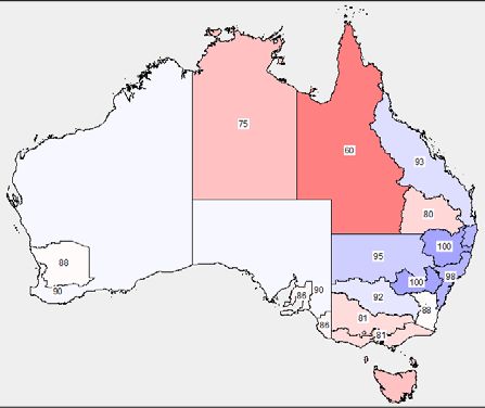
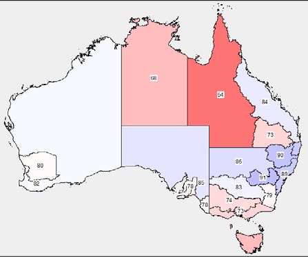
16

Appendix A: maps of historical rainfall and temperature variation and
accompanying agricultural productivity levels
Figure A1: Regions of VU-TERM in this study*

 RoA

 OutbackQld
 ECoastQld

 RoWA

 DDw mMnGBQld

 EyreMallOBSA New EngNWGrft
 FarWestOrana
 WheatInldWA
 CoastNSW
 CentralWest
 AdelCstSA RvnMurray
 CapitalReg
 NthAndCntVic
 AdelCstSA
 RoVic

*Rest of Australia (RoA) includes Tasmania. Tasmania’s rainfall and temperature anomalies
determine the region’s productivity levels.

Figure A2: Agriculture as % of regional GDP

 1.7

 16.2
 1.6

 14.6

 10.1
 10.4
 24.5
 0.3
 5.9
 1.1 2.7 11.2
 16.6
 3.0
 12.9
 2.7
 1.9
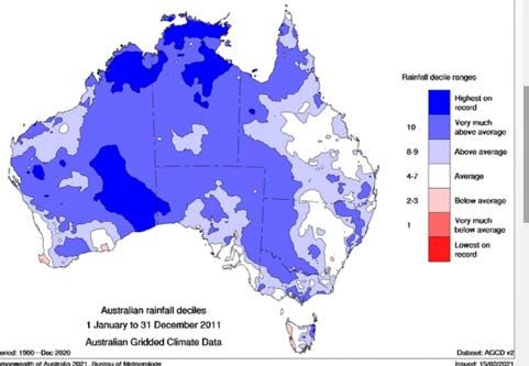
17

Figure A3: Rainfall & temperature Seasonal index year 1 “2020”= 2016-17
anomalies and consequent farm
productivity levels

Year 1 (2016)

 “2030” yr 1

Winter rain year (2016):

 101

 99
 87

 93

 99

 102 101
 101
 91
 98
 109
 102 105
 108
 100
 102
 104

Mean temperature anomaly year 1:
 “2050” yr 1
18

Figure A3 (cont.): Seasonal index year 2 all runs= 2017-18

Winter rain year 2:

Mean temperature anomaly year 2:
19

Figure A3 (cont.): Seasonal index year 3 all runs= 2018-19

Year 3 (2018)

Winter rain year 3:

Mean temperature anomaly year 3:
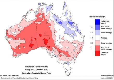
20

Figure A3 (cont.):
Year 4(2019) Seasonal index year 4 all runs= 2019-20

Winter rain year 4:

Mean temperature anomaly year 4:
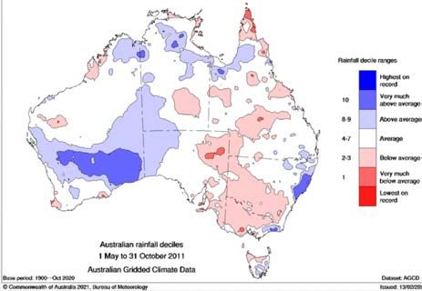
21

Figure A3 (cont.):
Year 5 (2020) Seasonal index year 5 “2020”= 2020-21

Winter rain year 5:

 “2030” yr 5

Mean temperature anomaly year 5:

 “2050” yr 5
22

Figure A3 (cont.):
Year 6 based on 2011 Seasonal index year 6 all runs

Winter rain year 6:

Mean temperature anomaly year 6:
23

Figure A3 (cont.): Seasonal index year 7 “2020”

Year 7 based on 2012

Winter rain year 7:

 “2030” yr 7

Mean temperature anomaly year 7:

 “2050” yr 7
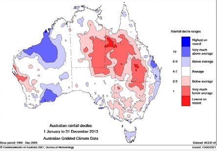
24

Figure A3 (cont.):
Year 8 based on 2013 Seasonal index year 8 all runs

Winter rain year 8:

Mean temperature anomaly year 8:
25

Figure A3 (cont.):
Year 9 based on 2014 Seasonal index year 9 “2020”

Winter rain year 9: “2030” yr 9

Mean temperature anomaly year 9: “2050” yr 9
26

Figure A3 (cont.): Seasonal index year 10 “2020”

Year 10 based on 2015

Winter rain year 10: “2030” yr 10

Mean temperature anomaly year 10:

 “2050” yr 10
27

Appendix B: General information on VU-TERM
What is a computable general equilibrium (CGE) model?
A CGE model can be an economy-wide model. In the context of VU-TERM, it is an economy-wide
model that also includes small-region representation. Unlike an input-output model which solves either
for quantities or for prices, but not both at once, a CGE model solves for both prices and quantities
together.
CGE models can be either comparative static or dynamic. Comparative static models are easier to run
than dynamic models. However, comparative static results are in some respects harder to explain.
Results are reported as changes from a base case – at some point in the future. The only base case
defined in a comparative static model is the initial database.
In dynamic models, we prepare a forecast baseline. This may include forecast increases in
macroeconomic variables, technological change and taste changes. For example, agricultural
productivity historically has grown by 1 to 2% per annum, so productivity growth of this magnitude is
imposed on the forecast baseline.
When we report results in a dynamic model, they are as cumulative deviations from the forecast
baseline. That is, the modelled impacts of a farm productivity study will be the marginal contribution
of productivity shocks ascribed in addition to those of the forecast baseline.

Dynamic CGE modelling
Dynamic models trace the effects of ascribed direct impacts across time periods. The theoretical basis
of dynamics is in linkages between investment and capital across time, and the balance of trade and net
foreign liabilities. Investment and balance of trade outcomes are flows that a comparative static model
includes. Capital and net foreign liabilities are stocks that require a dynamic model.
Dynamic VU-TERM combines much of the theory of dynamic national models (see Dixon and Rimmer,
2002) with bottom-up, regional representation. That is, each region in VU-TERM has its own
production functions, household demands, input-output database and inter-regional trade matrices
(Figure A1 is a map of regions for which individual representation is possible). This enables us to model
relatively local issues.

Dynamic VU-TERM
TERM was originally developed by Mark Horridge at the Centre of Policy Studies
(see https://www.copsmodels.com/term.htm). Since then, Glyn Wittwer has developed a
dynamic version of the model, an application of which Wittwer et al. (2005) is an example.
In dynamic VU-TERM, we use an underlying forecast. This may be based on the macro forecasts of
other agencies. The underlying forecast or baseline gives us a year-by-year “business as usual” case.
Typical variables to be reported in the policy scenario relative to a baseline forecast are regional real
GDP, employment and aggregate consumption. Industry level results are also available.

Labour market – forecast v. policy scenario
In the theory of regional labour market adjustment, if regional labour market conditions
improve or deteriorate relative to forecast, adjustment occurs in the short term mainly via
changes in employment. Regional wages adjust sluggishly, with gradual adjustment in regional
labour market supply (i.e., through migration between regions). Real wages will fall or rise to
close the gap between employment and slowly adjusting labour supply. Once the deviation in
employment is equal to the deviation in labour supply, real wages reach a turning point (either
they bottom out, in the case of a weakening labour market, or peak, in the case of strengthened
28

labour market conditions). Within this theory, adjustment in the longer term occurs via a
combination of altered regional labour supply and real wages that deviate relative to those in
other regions. Figure A3 shows an example, in which weakened labour market conditions in a
region lead to unemployment in the short run and a lower real wage in the region in the long
run.
Figure A1: An example of a weakened regional labour market with eventual recovery
(% change from forecast)

 0.2
 Employment

 0
 2005 2008 2011 2014 2017 2020 2023
 -0.2 Labour supply

 -0.4

 -0.6
 Real wage
 -0.8

 -1

Production technologies
VU-TERM contains variables describing: primary-factor and intermediate-input-saving
technical change in current production; input-saving technical change in capital creation; and
input-saving technical change in the provision of margin services (e.g. transport and retail
trade).
VU-TERM’s unique treatment of transport to assess the regional benefits of the project
The supply of margins originating in one region can lower the costs of moving goods between
regions further afield. Previous multi-regional models assign the margins supply of a sale either
to the origin or destination of the sale.
GEMPACK software
Dynamic VU-TERM uses GEMPACK software for implementation (Horridge, et al. 2018).

References and examples of published applications
Dixon, P.B. and Rimmer, M.T. (2002). Dynamic General Equilibrium Modelling for
Forecasting and Policy: a Practical Guide and Documentation of MONASH, Contributions to
Economic Analysis 256, North-Holland, Amsterdam.
29

Dixon, P., Rimmer, M. and Wittwer, G. (2011), “Saving the Southern Murray-Darling Basin:
the Economic Effects of a Buyback of Irrigation Water”, Economic Record, 87(276): 153-168.
Horridge, M, Madden, J. & Wittwer, G. (2005). Using a highly disaggregated multi-regional
single-country model to analyse the impacts of the 2002-03 drought on Australia. Journal of
Policy Modelling, 27, 285-308.
Horridge J.M., Jerie M., Mustakinov D. & Schiffmann F. (2018), GEMPACK manual,
GEMPACK Software, ISBN 978-1-921654-34-3
Wittwer, G., Vere, D., Jones, R. and Griffith, G. (2005), “Dynamic general equilibrium analysis
of improved weed management in Australia's winter cropping systems”, Australian Journal of
Agricultural and Resource Economics, 49(4): 363-377, December.
Wittwer, G. (2009), “The economic impacts of a new dam in South-east Queensland”,
Australian Economic Review, 42(1):12-23, March.
Wittwer, G. and Griffith, M. (2011), “Modelling drought and recovery in the southern Murray-
Darling basin”, Australian Journal of Agricultural and Resource Economics, 55(3): 342-359.
Wittwer, G., McKirdy, S. and Wilson, R. (2005), “The regional economic impacts of a plant
disease incursion using a general equilibrium approach”, Australian Journal of Agricultural
and Resource Economics 49(1): 75-89, March.
Wittwer, G. (2012) (editor), Economic Modeling of Water: The Australian CGE Experience,
Springer, Dordrecht, Netherlands (186 pages).
Wittwer, G. (2014), “Modelling the economic impacts of changing SA Water’s pricing. Report
prepared for the Essential Services Commission of South Australia.” Downloadable at
http://www.escosa.sa.gov.au/library/140711-WaterInquiry-
ModellingEconomicImpactsChangingPricing-VicUni-ConsultantReport.pdf.
You can also read