Moving object recognition system on a pedestrian crossing - IOPscience
←
→
Page content transcription
If your browser does not render page correctly, please read the page content below

Journal of Physics: Conference Series

PAPER • OPEN ACCESS

Moving object recognition system on a pedestrian crossing
To cite this article: E I Semenova et al 2021 J. Phys.: Conf. Ser. 1728 012004

View the article online for updates and enhancements.

                               This content was downloaded from IP address 46.4.80.155 on 31/01/2021 at 15:02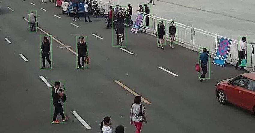
CEQCL 2020                                                                                                      IOP Publishing
Journal of Physics: Conference Series                         1728 (2021) 012004          doi:10.1088/1742-6596/1728/1/012004

Moving object recognition system on a pedestrian crossing

                     E I Semenova1, Sh D Kyarimova1, V V Kukartsev1,2, A A Leonteva2, A R Ogol1 and
                     A S Bondarev1
                     1
                       Reshetnev Siberian State University of Science and Technology, 31 Krasnoyarsky
                     Rabochy Av., Krasnoyarsk, 660037, Russian Federation
                     2
                       Siberian Federal University, 79 Svobodny pr., Krasnoyarsk, 660041, Russian
                     Federation

                     E-mail: vlad_saa_2000@mail.ru

                     Abstract. The article discusses the development of a system for recognizing people at a
                     pedestrian crossing. The recognition system includes a trained classifier and two sets of images
                     taken from an open database containing images of city streets from outdoor cameras. Input
                     information prepared using PictureCropper application. The classifier was tested based on the
                     prepared sets of images. The result is shown in the figure, and after testing, the metrics were
                     calculated, necessary to assess the effectiveness of the resulting classifier for each set. System is
                     being developed for specialists, which will allow individual and centralized adjustment of the
                     adjustment of pedestrian phases for each road situation, both for the local system of controllers,
                     and in accordance with the existing algorithms of coordination systems with the expansion of
                     such.

1. Introduction
The functioning of urban life in accordance with the development of technological capabilities is
undergoing significant changes [1, 2]. First of all, this concerns the implementation of software and
hardware solutions that allow the transition to centralized management with minimal or complete
absence of human management. One of the central areas of activity of any city is traffic regulation
[3 - 5].
    At the moment, traffic cameras have a certain distribution, the range of tasks of which is quite wide:
from fixing traffic violations to analyzing traffic flow using detection systems. In the general case, the
named traffic flow solved by artificial intelligence, as such, is the central issue of road functioning.
However, the application of the detection system is also advisable in the case of pedestrian traffic as a
full-fledged road user [6, 7].
    With well-calculated cycles, the traffic load will decrease if the proposed system is used in
collaboration with traffic lights. Switching to the green signal of a pedestrian traffic light will be made
not only during a certain phase of movement, but also in the presence of a pedestrian in the frame
[8, 9].
    Thus, in the absence of pedestrian traffic, the traffic flow is automated, without the participation of
the dispatcher, additional time will be presented on the basis of the information received by the proposed
system, which indicates a high rate of adaptability of the process to the situation in real time [3, 7, 10].

              Content from this work may be used under the terms of the Creative Commons Attribution 3.0 licence. Any further distribution
              of this work must maintain attribution to the author(s) and the title of the work, journal citation and DOI.
Published under licence by IOP Publishing Ltd                          1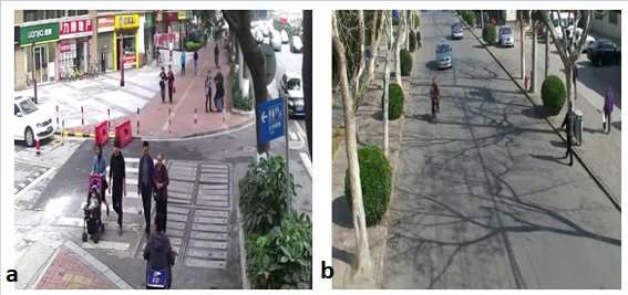
CEQCL 2020                                                                                 IOP Publishing
Journal of Physics: Conference Series          1728 (2021) 012004    doi:10.1088/1742-6596/1728/1/012004

2. Pedestrian crossing person recognition system
During the development of any system using the Viola-Jones method, it is necessary to carefully
approach the selection of test data, since the formed sample of images directly affects the quality of the
recognition model.
   An open for use database was used, containing 5759 images of city streets from outdoor video
surveillance cameras. The photos were taken from different devices and in different parts of the city.
Examples of images are shown in Figure 1.

             Figure 1. Prepared images.

    To train the classifier, it is necessary to prepare two training sets of images: positive and negative.
The positive set contains images of the object (pedestrian), which the classifier needs to learn to detect.
The negative set, on the other hand, contains images of the background without the desired object, that
is, in this case, a photo of streets without pedestrians.
    Both sets were prepared manually from a selected database using the open source PictureCropper
application, which allows you to select and save as separate images the required areas in the pictures.
The work resulted in 1,892 images of pedestrians and 5,598 “non-pedestrians” in BMP format.
    For each set, a text file was generated containing information about the images. Description files
have different structures. The description file for negative examples contains a list of relative paths to
the corresponding images. The description file for positive examples, in addition to the list of relative
paths to the corresponding images, should contain: the number of objects to be found in the image, their
position on the image and size. Taking into account that each positive image is actually the desired
object, the coordinates of their position are [0, 0], and their size is the size of the image itself.
    The final preparation step before starting the training is to convert all positive images to a common
format. For this, the opencv_createsamples tool implemented in the OpenCV library was used. It has
several purposes, including generating multiple samples from one given positive image by distorting it,
however, in this case, it was used exclusively for converting to a common 10-by-30 pixel format and
recording a collection of the resulting images in vector format.
    Below is the result of the work. Arguments given:

   •    File name for recording (-vecsamples.vec).
   •    Maximum angles of rotation for distortion (-maxxangle 0, -maxyangle 0, -maxzangle 0).
   •    The number of required samples, the same as the number of positive images (-num 1892).
   •    Size of the template to which the images are converted, in pixels (-w, -h).

                                                     2
CEQCL 2020 IOP Publishing
Journal of Physics: Conference Series 1728 (2021) 012004 doi:10.1088/1742-6596/1728/1/012004
The cascade is trained using the implemented algorithm of the OpenCV library opencv_traincascade.
Arguments given:
• Storage path of layers and cascade (-datahaarcascade).
• Vector file with positive images (-vecsamples.vec).
• Negative images description file (-dg ).
• Number of training layers (-numStages 20).
• Number of positive / negative images used in the training process for each layer (-numPos 1600
–numNed 5592).
• Size of the template to which the images were reduced, in pixels (- w, - h).
• Type of Haar feature set used in training (-modeALL).
• The amount of allocated memory for the pre-calculated values of features, MB (-
precalcValBufSize4096).
• The amount of allocated memory for the pre-calculated feature indices, MB (-
precalcIdxBufSize4096).
With the beginning of training, the output of training results for each layer of the cascade to the
console is provided. An example of such results is shown in tables 1-3. An important indicator is FA
(FalseAlarm) - the level of false alarms, showing the activation of the training classifier to false objects,
that is, the detection error. When the default threshold 0.5 is reached, the classifier layer ends training.
Below is the learning process for the first, second and third layers.
1st layer:
TRAINING 1-stage
TRAINING 2–stage
TRAINING 3-stage
The results of each layer are presented consequently in tables 1, 2 and 3.
3CEQCL 2020 IOP Publishing
Journal of Physics: Conference Series 1728 (2021) 012004 doi:10.1088/1742-6596/1728/1/012004
Table 1. First layer results.
N HR FA
1 1 1
2 1 1
3 1 1
4 1 1
5 1 1
6 1 1
7 1 1
8 0.9975 0.776288
9 0.996875 0.764843
10 0.99625 0.531831
11 0.99625 0.519134
12 0.995625 0.449034
Table 2. Second layer results.
N HR FA
1 1 1
2 1 1
3 1 1
4 1 1
5 1 1
6 0.99875 0.920243
7 0.99625 0.864807
8 0.99625 0.801502
9 0.99625 0.790236
10 0.99625 0.730508
11 0.995625 0.70422
12 0.995625 0.655579
13 0.995625 0.588877
14 0.99625 0.55794
15 0.995625 0.531652
16 0.995625 0.511803
17 0.995625 0.519134
18 0.995625 0.443491
4CEQCL 2020 IOP Publishing
Journal of Physics: Conference Series 1728 (2021) 012004 doi:10.1088/1742-6596/1728/1/012004
Table 3. Third layer results
N HR FA
1 1 1
2 1 1
3 1 1
4 1 1
5 1 1
6 1 1
7 0.995625 0.95583
8 0.996875 0.903076
9 0.996875 0.865522
10 0.99625 0.882332
11 0.995625 0.829399
12 0.995625 0.853362
13 0.995625 0.861946
14 0.995625 0.817239
15 0.995625 0.770744
16 0.995625 0.742847
17 0.995625 0.731402
18 0.995625 0.686159
19 0.995625 0.646102
20 0.995625 0.655222
21 0.995625 0.634835
22 0.995625 0.575107
23 0.995625 0.555257
24 0.995625 0.529149
25 0.995625 0.499106
3. Testing a trained classifier
Upon completion of training, the classifier is tested, and then its effectiveness is assessed.
For testing, it is necessary to prepare a sample of images with known information about each image:
• The presence or absence of the desired object.
• The number of searched objects, if any.
• Number of third-party objects.
Test sets of images were prepared for testing. We used only those images that were not included in
the training set. The sets were compiled based on the presence of the following objects in the image:
• Upright person.
• A person in a sitting position.
5CEQCL 2020 IOP Publishing
Journal of Physics: Conference Series 1728 (2021) 012004 doi:10.1088/1742-6596/1728/1/012004
• Partial visibility of a person.
• Person with a vehicle.
Additionally, a set of images was prepared, in which not a single person was present.
Partial visibility - the covering of a part of a person's figure either by a third-party object of the
environment, or by another person. In this case, the ability to recognize a pedestrian in a crowd of other
people is considered. Vehicles are those vehicles that can be used by a person on a pedestrian zone in
compliance with traffic rules. Such means are bicycles, roller skates, scooters, skateboards and the like.
Each set consists of fifty images, so the total of all test images is 250 units.
A program for processing static images using the obtained classifier was implemented. A sequence
of static images is fed to the input of the program, each of which is processed by the classifier for the
presence of the desired objects (pedestrians). When the program is running, each image is displayed in
a separate window. If the classifier identifies an object, then on the image the program selects this object
according to the coordinates received from the classifier in a square frame. Isolation is performed for
visual assessment of the detection results. The transition to the processing of the next image is performed
by pressing the Enter key in the console window. The program will run until the last image in the
specified file folder is processed. An example of the program is shown in Figure 2.
Figure 2. Application result.
4. Calculation of metrics to assess the effectiveness of the classifier
The test results are a sample of values TP (truepositive - an object belonging to the class in question was
found), FN (falsenegative - an object belonging to the class in question was not found), TN (truenegative
- the classifier correctly asserts that the object does not belong to the class in question), FP (falsepositive
- an object was found that does not belong to the class in question) for each set.
The disparity matrix presented in Table 4 clearly demonstrates the essence of these indicators.
Table 4. Discrepancy matrix.
Belongs to class (Р) Does not belong to class (N)
Class membership predicted TP FP
Lack of class membership TN
FN
predicted
Based on the obtained values, the following simple statistics can be obtained: accuracy, precision
(precision), recall (recall) and F-measure (F-measure).
Accuracy is a widely used and easy to understand metric. This is the ratio of all correctly recognized
objects to the total number of all classifications.
6CEQCL 2020 IOP Publishing
Journal of Physics: Conference Series 1728 (2021) 012004 doi:10.1088/1742-6596/1728/1/012004
= , (1)
Precision - the proportion of correctly recognized objects among all objects selected by the classifier.
= , (2)
Recall - the proportion of classified search objects to the total number of search objects, that is, how
well the classifier finds objects from the class. The higher the completeness value, the fewer positive
examples are missed in the classification.
= . (3)
The Specificity shows the proportion of correct responses of the classifier to the total number of
objects that are not the desired ones, that is, how often the classifier does not correctly assign objects to
the class.
= . (4)
F-measure - weighted harmonic mean of completeness and accuracy. This indicator demonstrates
how many cases the classifier predicts correctly, and how many true instances the classifier will not
miss.
∗ "# #$%∗& " ''
= "# #$% & " ''
. (5)
An important note is that TP and FN values for each sample are determined according to the
previously described features of the image set.
For example, if a partially visible pedestrian is present in an image in a set with erect pedestrians,
then he is not included in the accounting of these indicators.
The obtained indicators of the kits are presented in table 5.
Table 5. Detection test metrics.
TP FN TN FP
Upright 154 41 385 8
Sitting 6 78 401 11
Partial visibility 10 132 329 15
With a vehicle 97 34 298 5
Absent - - 303 6
Using the obtained values for each sample by formulas 1 - 5, the metrics were calculated, which are
necessary to assess the efficiency of the obtained classifier for each set. The results for each metric and
their analysis are shown below.
Figure 3 shows a graphical ratio of correct answers to the total number of all classifications. As can
be seen from the diagram, the classifier has a small proportion of correct recognition of seated and
partially obstructed people.
7CEQCL 2020 IOP Publishing
Journal of Physics: Conference Series 1728 (2021) 012004 doi:10.1088/1742-6596/1728/1/012004
Figure 3. F-measure for different types of set.
Although this indicator is not fully informative, it can already be concluded that it is potentially good
at working with images in which people are captured in full growth and with vehicles, since this
parameter exceeds 90%.
Further, the recognition accuracy was calculated. Accuracy is the likelihood that the classifier will
identify the person as a pedestrian rather than the background of the image. As can be seen in Figure 3,
the classifier “will not see” a person sitting or a person in a crowd (less than 40%). At the same time,
the chances of mistaking a standing person or a person on a bicycle for a third-party object are extremely
small (less than 5%).
Completeness and specification are closely related metrics: completeness shows how many
pedestrians were found to the actual number of pedestrians. The specificity, on the contrary,
demonstrates the relationship of the correct definition of the background to the total number of such
third-party objects. As with the previously reviewed diagrams, the diagram in Figure 6 demonstrates a
critically low chance of detecting the same subcategories of pedestrians. We can say that the classifier
does not detect such pedestrians at all. However, the probability of false positives for all sets is less than
5%, as shown in Figure 3. This is a very good indicator for the problem being solved.
The F-score is the final measure of the efficiency of the classifier. It links the accuracy and
completeness of detection. In other words, this indicator demonstrates how many cases the classifier
predicts correctly, and how many true instances it will not miss. Figure 4 clearly confirms the
inexpediency of using the classifier to detect seated people and people whose figure is not fully
displayed. However, on the contrary, the classifier copes well with the task of detecting the other two
categories, demonstrating an F-measure value of more than 80%.
Based on the test results, the following conclusions were made:
• The classifier does not recognize people whose figure is covered by third-party objects of the
environment by more than 50%.
• The classifier does not recognize people in motion (blurred image).
• The classifier poorly recognizes people who are far from the actual location of the shooting
device.
• The classifier poorly recognizes seated people.
• The classifier successfully recognizes full height people and cyclists.
8CEQCL 2020 IOP Publishing
Journal of Physics: Conference Series 1728 (2021) 012004 doi:10.1088/1742-6596/1728/1/012004
The second and third points are not disadvantaging of the classifier within the framework of the
problem being solved. First, in the general case, a person who needs to cross a road section stands
motionless, so the classifier is not tasked with detecting a person who is moving quickly. Secondly, a
person must be close to a pedestrian crossing, therefore, taking into account the system's requirement
for a CCTV camera (or other recording device) above the pedestrian zone, the inability to recognize
people far away is rather a positive characteristic of the classifier.
These tests were performed to assess the classifier's ability to recognize all common types of
pedestrians. In this case, the types of pedestrians mean dividing people into categories according to their
location in the frame and relative to their surroundings. However, to assess the efficiency of the classifier
within the framework of the problem being solved, not all data obtained as a result of testing will be
used: only erect pedestrians and pedestrians with vehicles will be taken into account. The reasons for
excluding other types are as follows:
• The system is not faced with the task of detecting seated people, since it is assumed that to cross
a pedestrian crossing, a person must stand directly or near the road: this condition will exclude
errors in recognizing people sitting on benches near the crossing as those who want to cross the
road.
• The condition of the location of the camera ensures that a person completely enters the lens.
Estimates of the identification of erect pedestrians and pedestrians with vehicles are presented in
Figure 4.
Figure 4. Final assessments of the classifier.
There is a certain probability (less than 30%) that the classifier will not “see” a pedestrian, but this
probability is acceptable. More important characteristics are specification and accuracy, which
demonstrate the minimum (less than 5%) chances of the system transmitting false signals (in the absence
of a pedestrian in the frame) about the need to switch pedestrian traffic lights.
5. Conclusion
As a result of this work, a system for recognizing people in images and video sequences in real time at
a pedestrian crossing was created. To implement the classifier, the methods of object detection were
considered and the Viola-Jones method was selected for the most suitable for the specifics of the task at
hand, and the resulting classifier was evaluated and an application was implemented for processing the
9CEQCL 2020 IOP Publishing
Journal of Physics: Conference Series 1728 (2021) 012004 doi:10.1088/1742-6596/1728/1/012004
video stream in real time using the obtained classifier. Analysis of the experimental results allows us to
speak about the successful operation of the system in recognizing pedestrians.
The developed system is primarily intended for the optimization and regulation of road traffic.
References
[1] Datola G, Bottero M and De Angelis E 2020 Addressing Social Inclusion Within Urban
Resilience: A System Dynamics Approach In: INTERNATIONAL SYMPOSIUM: New
Metropolitan Perspectives pp 510-9
[2] Dong C Z, Bas S and Catbas F N 2020 A portable monitoring approach using cameras and
computer vision for bridge load rating in smart cities Journal of Civil Structural Health
Monitoring 10(5) 1001-21
[3] Oc T and Tiesdell S 1998 City centre management and safer city centres: approaches in Coventry
and Nottingham Cities 15(2) 85-103
[4] Obedin A V, Soroka E O, Kukartsev V V, Mikhalev A S, Tynchenko V S, Semenova E I and
Bashmur K A 2019 The developing program system of social monitoring of road improvement
and urban infrastructure Journal of Physics: Conference Series 1399(5) 055021
[5] Oc T and Tiesdell S 1999 The fortress, the panoptic, the regulatory and the animated: Planning
and urban design approaches to safer city centres Landscape Research 24(3) 265-86
[6] Ballesteros J, Rahman M, Carbunar B and Rishe N 2012 Safe cities. A participatory sensing
approach In: 37th Annual IEEE Conference on Local Computer Networks pp 626-34
[7] Tubaishat A and Elsayed R 2017 Safe city: Introducing a flawless model and implementation
guidelines to reduce crime rate and response time In: Proceedings of the 29th International
Business Information Management Association Conference - Education Excellence and
Innovation Management through Vision 2020: From Regional Development Sustainability to
Global Economic Growth 474-85
[8] Li Y H, Zhang X D, Feng Z C and Luan Z H 2014 Research on the Key Equipment Performance
of Stage Video Surveillance and Scheduling System Based on IP Network Applied Mechanics
and Materials 644 957-60
[9] Zeng X, Guo H and Hu W 2019 Design and Implementation of Shipping Video Surveillance
Equipment Based on Raspberry Pi In: 2019 IEEE International Conference on Computational
Science and Engineering (CSE) and IEEE International Conference on Embedded and
Ubiquitous Computing (EUC) pp 66-70
[10] Pan X, Hu H, Xu J and Li M 2020 Research on Video Surveillance Robot Based on SSH Reverse
Tunnel Technology In: 2020 3rd International Conference on Advanced Electronic Materials,
Computers and Software Engineering (AEMCSE) pp 298-302
10You can also read