Multi-Slice Fusion for Sparse-View and Limited-Angle 4D CT Reconstruction
←
→
Page content transcription
If your browser does not render page correctly, please read the page content below
448                                                                                        IEEE TRANSACTIONS ON COMPUTATIONAL IMAGING, VOL. 7, 2021

                    Multi-Slice Fusion for Sparse-View and
                    Limited-Angle 4D CT Reconstruction
           Soumendu Majee , Student Member, IEEE, Thilo Balke, Student Member, IEEE, Craig A. J. Kemp,
                   Gregery T. Buzzard , Member, IEEE, and Charles A. Bouman , Fellow, IEEE

   Abstract—Inverse problems spanning four or more dimensions
such as space, time andother independent parameters have become
increasingly important. State-of-the-art 4D reconstruction meth-
ods use model based iterative reconstruction (MBIR), but depend
critically on the quality of the prior modeling. Recently, plug-and-
play (PnP) methods have been shown to be an effective way to
incorporate advanced prior models using state-of-the-art denoising
algorithms. However, state-of-the-art denoisers such as BM4D and
deep convolutional neural networks (CNNs) are primarily available
for 2D or 3D images and extending them to higher dimensions is
difficult due to algorithmic complexity and the increased difficulty
of effective training. In this paper, we present multi-slice fusion, a
novel algorithm for 4D reconstruction, based on the fusion of mul-
tiple low-dimensional denoisers. Our approach uses multi-agent
consensus equilibrium (MACE), an extension of plug-and-play, as a
framework for integrating the multiple lower-dimensional models.
                                                                                Fig. 1. Illustration of our multi-slice fusion approach. Each CNN denoiser
We apply our method to 4D cone-beam X-ray CT reconstruction for
                                                                                operates along the time direction and two spatial directions. We fuse the CNN
non destructive evaluation (NDE) of samples that are dynamically                denoisers with the measurement model to produce a 4D regularized reconstruc-
moving during acquisition. We implement multi-slice fusion on                   tion.
distributed, heterogeneous clusters in order to reconstruct large
4D volumes in reasonable time and demonstrate the inherent par-
allelizable nature of the algorithm. We present simulated and real
experimental results on sparse-view and limited-angle CT data to                5D problems representing space-time and, for example, heart or
demonstrate that multi-slice fusion can substantially improve the               respiratory phase [1]–[6].
quality of reconstructions relative to traditional methods, while also             These higher-dimensional reconstruction problems pose sur-
being practical to implement and train.
                                                                                prisingly difficult challenges computationally and perhaps more
   Index Terms—Inverse problems, 4D tomography, Model based                     importantly, in terms of algorithmic design and training due to
reconstruction, Plug-and-play, Deep neural networks.                            the curse of dimensionality [7]. However, the high dimension-
                                                                                ality of the reconstruction also presents important opportunities
                                                                                to improve reconstruction quality by exploiting the regularity
                           I. INTRODUCTION                                      in the high-dimensional space. In particular, for time-resolved
    MPROVEMENTS in imaging sensors and computing power                          imaging, we can exploit the regularity of the image to reconstruct
I   have made it possible to solve increasingly difficult recon-
struction problems. In particular, the dimensionality of recon-
                                                                                each frame with fewer measurements and thereby increase tem-
                                                                                poral resolution. In the case of 4D CT, the contributions of [2],
struction problems has increased from the traditional 2D and                    [8], [9] have increased the temporal resolution by an order of
3D problems representing space to more difficult 4D or even                     magnitude by exploiting the space-time regularity of objects
                                                                                being imaged. These approaches use model-based iterative re-
                                                                                construction (MBIR) [10], [11] to enforce regularity in 4D using
   Manuscript received July 30, 2020; revised December 1, 2020 and February
19, 2021; accepted April 14, 2021. Date of publication April 21, 2021; date     simple space-time prior models. More recently, deep learning
of current version May 14, 2021. This work was supported by Eli Lilly and       based post-processing for 4D reconstruction has been proposed
Company under research project funding agreement under Grant 17099289.          as a method to improve reconstructed image quality [12].
Charles A. Bouman and Gregery T. Buzzard were supported in part by NSF
under Grant CCF-1763896. (Corresponding author: Soumendu Majee.)                   Recently, it has been demonstrated that plug-and-play (PnP)
   Soumendu Majee, Thilo Balke, and Charles A. Bouman are with the              priors [13]–[16] can dramatically improve reconstruction quality
School of Electrical and Computer Engineering, Purdue University, West          by enabling the use of state-of-the-art denoisers as prior models
Lafayette, IN 47907 USA (e-mail: smajee@purdue.edu; tbalke@purdue.edu;
bouman@purdue.edu).                                                             in MBIR. So PnP has great potential to improve reconstruction
   Craig A. J. Kemp is with Eli Lilly and Company, Indianapolis, IN 46225 USA   quality in 4D CT imaging problems. However, state-of-the-art
(e-mail: kemp_craig_a@lilly.com).                                               denoisers such as deep convolutional neural networks (CNN)
   Gregery T. Buzzard is with the Department of Mathematics, Purdue Univer-
sity, West Lafayette, IN USA (e-mail: buzzard@purdue.edu).                      and BM4D are primarily available for 2D and sometimes 3D
   Digital Object Identifier 10.1109/TCI.2021.3074881                           images, and it is difficult to extend them to higher dimensions [7],
                        2333-9403 © 2021 IEEE. Personal use is permitted, but republication/redistribution requires IEEE permission.
                                      See https://www.ieee.org/publications/rights/index.html for more information.

           Authorized licensed use limited to: Purdue University. Downloaded on May 20,2021 at 16:36:28 UTC from IEEE Xplore. Restrictions apply.
MAJEE et al.: MULTI-SLICE FUSION FOR SPARSE-VIEW AND LIMITED-ANGLE 4D CT RECONSTRUCTION                                                                       449

[17], [18]. In particular, extending CNNs to 4D requires very
computationally and memory intensive 4D convolution applied
to 5D feature tensor structures. This problem is further com-
pounded by the lack of GPU accelerated routines for 4D convolu-
tion from major Deep-Learning frameworks such as Tensorflow,
Keras, PyTorch 1 . Furthermore, 4D CNNs require 4D ground
truth data to train the PnP denoisers, which might be difficult or
impossible to obtain.
   In this paper, we present a novel 4D X-ray CT reconstruc-
tion algorithm that combines multiple low-dimensional CNN
denoisers to implement a highly effective 4D prior model.
Our approach, multi-slice fusion, integrates the multiple low-
dimensional priors using multi-agent consensus equilibrium
(MACE) [19]. MACE is an extension of the PnP framework
that formulates the inversion problem using an equilibrium
equation—as opposed to an optimization—and allows for the
use of multiple prior models and agents.
   Fig. 1 illustrates the basic concept of our approach. Multi-slice
fusion integrates together three distinct CNN denoisers each of
                                                                               Fig. 2. Illustration of 4D cone-beam X-ray CT imaging. The dynamic object
which is trained to remove additive white Gaussian noise along                 is rotated and several 2D projections (radiographs) of the object are measured
lower dimensional slices (hyperplanes) of the 4D object. When                  for different angles. The projections are divided into Nt disjoint subsets for each
MACE fuses the denoisers it simultaneously enforces the con-                   of the Nt time-points.
straints of each denoising agent, so that the reconstructions are
constrained to be smooth in all four dimensions. Consequently,                 we introduce the theory behind MACE model fusion. In Sec-
multi-slice fusion results in high-quality reconstructions that are            tion IV, we use the MACE framework to introduce multi-slice fu-
practical to train and compute even when the dimensionality of                 sion. In Section V, we describe our training pipeline for training
the reconstruction is high. In our implementation, one MACE                    the CNN denoisers. In Section VI, we describe our distributed
agent estimates the cone-beam tomographic inversion. The re-                   implementation of multi-slice fusion on heterogeneous clusters.
maining 3 agents are CNN denoisers trained to remove additive                  Finally, in Section VII, we present results on sparse-view and
white Gaussian noise along two spatial directions and the time                 limited-angle 4D CT using both simulated and real data.
direction. The CNN agents work along complimentary spatial
directions and are designed to take as input a stack of five 2D                                      II. PROBLEM FORMULATION
slices from five neighboring time-points. We refer to this as 2.5D
                                                                                  In 4D X-ray CT imaging, a dynamic object is rotated and
denoising [7], [20]. Further details are given in Section IV.
                                                                               several 2D projections (radiographs) of the object are measured
   The MACE solution can be computed using a variety of
                                                                               for different angles as illustrated in Fig. 2. The problem is then
algorithms, including variants of the plug-and-play algorithm
                                                                               to reconstruct the 4D array of X-ray attenuation coefficients
based on ADMM or other approaches [13], [14], [21], [22].
                                                                               from these measurements, where three dimensions correspond
We implement multi-slice fusion on distributed heterogeneous
                                                                               to the spatial dimensions and the fourth dimension corresponds
clusters in which different agent updates are distributed onto
                                                                               to time.
different cluster nodes. In particular, the cone-beam inversion
                                                                                  Let Nt be the number of time-points, Mn be the number
computations are distributed onto multiple CPU nodes and con-
                                                                               of measurements at each time-point, and Ns be the number of
currently, the CNN denoising computations are distributed onto
                                                                               voxels at each time-point of the 4D volume. For each time-point
multiple GPU nodes.
                                                                               n ∈ {1, . . . , Nt }, define yn ∈ RMn to be the vector of sinogram
   We present experiments using both simulated and real data
                                                                               measurements at time n, and xn ∈ RNs to be the vectorized
of 4D NDE tomographic imaging from sparse-views, and we
                                                                               3D volume of X-ray attenuation coefficients for that time-point.
compare multi-slice fusion with MBIR using total variation (TV)
                                                                               Let us stack all the measurements to forma measurement
and 4D Markov random field (MRF) priors. Our results indicate
                                                                               vector y = [y1 , .., yN
                                                                                                         t
                                                                                                           ] ∈ RM where M = N      n=1 Mn is the
                                                                                                                                    t

that multi-slice fusion can substantially reduce artifacts and
                                                                               total number of measurements. Similarly, let us stack the 3D
increase resolution relative to these alternative reconstruction
                                                                               volumes at each time-point to form a vectorized 4D volume x =
methods.
                                                                               [x                   N
                                                                                 1 , . . . , xNt ] ∈ R , where N = Nt Ns is the total number
   The rest of the paper is organized as follows. In Section II, we
                                                                               voxels in the 4D volume. The 4D reconstruction problem then
introduce the problem of 4D CT reconstruction. In Section III,
                                                                               becomes the task of recovering the 4D volume of attenuation
                                                                               coefficients, x, from the series of sinogram measurements, y.
                                                                                  In the traditional maximum a posteriori (MAP) approach, the
                                                                               reconstruction is given by
  1 Currently only 1D, 2D, and 3D convolutions are supported with GPU
acceleration                                                                                       x∗ = arg minx {l(x) + βh(x)}                               (1)

           Authorized licensed use limited to: Purdue University. Downloaded on May 20,2021 at 16:36:28 UTC from IEEE Xplore. Restrictions apply.
450                                                                                       IEEE TRANSACTIONS ON COMPUTATIONAL IMAGING, VOL. 7, 2021

where l(x) is the data-fidelity or log-likelihood term, h(x) is
the 4D regularizer or prior model, and the unit-less parameter
β controls the level of regularization in the reconstruction. The
data-fidelity term, l(x), can be written in a separable fashion as
                              Nt
                           1
                 l(x) =          yn − An xn 2Λn                       (2)
                           2 n=1

where An is the system matrix, and Λn is the weight matrix for
time-point n. The weight matrix accounts for the non-uniform                   Fig. 3. Illustration of consensus equilibrium as analogous to a force balance
noise variance due to a Gaussian approximation [23] of the                     equation: each agent pulls the solution toward its manifold and at equilibrium
underlying Poisson noise. The weight matrix is computed as                     the forces balance each other.
Λn = diag{c exp{−yn } where the scalar c is empirically cho-
sen [2].                                                                       operator F : R(K+1)N → R(K+1)N as
   If the prior model, h(x), can be expressed analytically like a                                        ⎡          ⎤
4D Markov random field (MRF) as in [2], [4], then the expression                                            L(W0 )
                                                                                                         ⎢ H1 (W1 ) ⎥
in equation (1) can be minimized iteratively to reconstruct the                                          ⎢          ⎥
                                                                                                         ⎢          ⎥
image. However, in practice, it can be difficult to represent an                                         ⎢          ⎥
                                                                                                F (W ) = ⎢     ..   ⎥,                                   (6)
advanced prior model in the form of a tractable cost function                                            ⎢      .   ⎥
                                                                                                         ⎢          ⎥
h(x) that can be minimized. Consequently, PnP algorithms                                                 ⎣          ⎦
have been created as a method for representing prior models                                                HK (WK )
as denoising operations [13], [14]. More recently, PnP methods
have been generalized to the multi-agent consensus equilibrium                 where W ∈ R(K+1)N is stacked representative variable. The
(MACE) framework as a way to integrate multiple models in a                    consensus equilibrium is the vector W ∗ ∈ R(K+1)N that satis-
principled manner [4], [19], [24].                                             fies
                                                                                                          F (W ∗ ) = G(W ∗ ),                            (7)
                   III. MACE MODEL FUSION
   In this section, we use the multi-agent consensus equilibrium               where G is an averaging operator given as
                                                                                                              ⎡ ⎤
(MACE) framework to fuse the data-fidelity term and multiple                                                     W
denoisers; these multiple denoisers form a single prior model for                                             ⎢ .. ⎥
                                                                                                              ⎢ ⎥
reconstruction. This allows us to construct a 4D prior model us-                                     G(W ) = ⎢ . ⎥ ,                                     (8)
                                                                                                              ⎣ ⎦
ing low-dimensional CNN denoisers (described in Section IV).
   To introduce the concept of consensus equilibrium, let us first                                               W
consider a variation of the optimization problem in equation (1)               and the weighted average is defined as
with K regularizers hk (x), k = 1, . . . , K. The modified opti-
                                                                                                                        K
mization problem can thus be written as                                                          1            β       1
                                                                                      W =          W0 +                 Wk .                           (9)
                                           K                                                   1+β          1+β K
              ∗                        β                                                                                          k=1
             x = arg minx l(x) +             hk (x)           (3)
                                      K                                        Notice the weighting scheme is chosen to balance the forward
                                              k=1
                                                                               and prior models. The unitless parameter β is used to tune the
where the normalization by K is done to make the regularization                weights given to the prior model and thus the regularization
strength independent of the number of regularizers.                            of the reconstruction. Equal weighing of the forward and prior
   Now we transform the optimization problem of equation (3)                   models can be achieved using β = 1.
to an equivalent consensus equilibrium formulation. However,                      If W ∗ satisfies the consensus equilibrium condition of equa-
in order to do this, we must introduce additional notation. First,             tion (7), then it can be shown [19] that W ∗ is the solution to
we define the proximal maps of each term in equation (3). We                   the optimization problem in equation (3). Thus if the agents in
define L(x) : RN → RN to be the proximal map of l(x) as                        MACE are true proximal maps then the consensus equilibrium
                                                                             solves an equivalent optimization problem.
                                         1           2
        L(x) = arg minz∈RN l(z) + 2 x − z2                  (4)                 However, if the MACE agents are not true proximal maps,
                                        2σ
                                                                               then there is no inherent optimization problem to be solved, but
for some σ > 0. Similarly, we define Hk (x) : RN → RN to be                    the MACE solution still exists. In this case, the MACE solution
the the proximal map of each hk (x), k = 1, . . . , K as                       can be interpreted as the balance point between the forces of each
                                                                             agent as illustrated in Fig. 3. Each agent pulls the solution toward
                                1           2
      Hk (x) = arg minz∈RN          x − z 2  +   h k (z)   . (5)             its manifold and the consensus equilibrium solution represents
                               2σ 2                                            a balance point between the forces of each agent. Thus MACE
Each of these proximal maps serve as agents in the MACE                        provides a way to incorporate non-optimization based models
framework. We stack the agents together to form a stacked                      such as deep neural networks for solving inverse problems.

          Authorized licensed use limited to: Purdue University. Downloaded on May 20,2021 at 16:36:28 UTC from IEEE Xplore. Restrictions apply.
MAJEE et al.: MULTI-SLICE FUSION FOR SPARSE-VIEW AND LIMITED-ANGLE 4D CT RECONSTRUCTION                                                              451

   To see how we can incorporate deep neural network based
                                                                                 Algorithm 1: Partial update Mann iteration for computing
prior models, first notice that equation (5) can be interpreted as
                                                                                 the MACE solution.
the MAP estimate for a Gaussian denoising problem with prior
model hk and noise standard deviation σ. Thus we can replace                        Input:Initial Reconstruction: x(0) ∈ RN
each MACE operator, Hk , for each k = 1, . . . , K in equation (5)                  Output:Final Reconstruction:
                                                                                                    ⎡ (0) ⎤        x∗
                                                                                                      x
with a deep neural network trained to remove additive white                                         ⎢     ⎥
Gaussian noise of standard deviation σ.                                               1 X ← W ← ⎣ ... ⎦;
   It is interesting to note that when Hk is implemented with                                         x(0)
a deep neural network denoiser, then the agent Hk is not, in                         2 whilenot convergeddo
general, a proximal map and there is no corresponding cost                           3 X ← F̃ (W ; X)
function hk . We know this because for Hk to be a proximal                           4 Z ← G(2X − W )
map, it must satisfy the condition that ∇Hk (x) = [∇Hk (x)]                         5 W ← W + 2ρ(Z − X)
(see [13], [25]), which is equivalent to Hk being a conservative                     6 x ∗ ← X0
vector function (see for example [26, Theorem 2.6, p. 527]).
For a CNN, ∇Hk is a function of the trained weights, and in
the general case, the condition will not be met unless the CNN
architecture is specifically designed to enforce such a condition.                Note that each Mann iteration update in equation (12) involves
   The consensus equilibrium equation 7 states the condition                   performing the minimization in equation (4). This nested itera-
that the equilibrium solution must satisfy. However, the ques-                 tion is computationally expensive and leads to slow convergence.
tion remains of how to compute this equilibrium solution. Our                  Instead of minimizing equation (4) till convergence, we initialize
approach to solving the consensus equilibrium equations is to                  with the result of the previous Mann iteration and perform only
first find an operator that has the equilibrium solution as a fixed            three iterations of iterative coordinate descent (ICD). We denote
point, and then use standard fixed point solvers. To do this, we               this partial update operator as L̃(W0 , X0 ) where X0 is the initial
first notice that the averaging operator has the property that                 condition to the iterative update. The corresponding new F
G(G(W )) = G(W ). Intuitively, this is true because applying                   operator approximation is then given by
averaging twice is the same as applying it once. Using this fact,
we see that                                                                                                         ⎡           ⎤
                                                                                                                   L̃(W0 ; X0 )
          (2G − I)(2G − I) = 4GG − 4G + I = I                         (10)                                       ⎢ H1 (W1 ) ⎥
                                                                                                                 ⎢              ⎥
where I is the identity mapping. We then rewrite equation (7) as                                                 ⎢              ⎥
                                                                                                                 ⎢              ⎥
                                                                                                    F̃ (W ; X) = ⎢      .       ⎥.                  (13)
                                                                                                                 ⎢      ..      ⎥
                                 F W ∗ = GW ∗                                                                    ⎢              ⎥
                                                                                                                 ⎣              ⎦
                       (2F − I)W ∗ = (2G − I)W ∗                                                                    Hk (WK )
            (2G − I)(2F − I)W ∗ = W ∗ .
So from this we see that the following fixed point relationship                   Algorithm 1 shows a simplified Mann iteration using partial
must hold for the consensus equilibrium solution.                              updates. We perform algebraic manipulation of the traditional
                                                                               Mann iterations [24], [27] in order to obtain the simplified but
                 (2G − I)(2F − I)W ∗ = W ∗ ,                          (11)     equivalent Algorithm III. It can be shown that partial update
                                                                               Mann iteration also converges [24], [27] to the fixed point in
and the consensus equilibrium solution W ∗ is a fixed point of
                                                                               equation (11). We used a zero initialization, x(0) = 0, in all our
the mapping T = (2G − I)(2F − I).
                                                                               experiments and continue the partial update Mann iteration until
   We can apply a variety of iterative fixed point algorithms
                                                                               the differences between state vectors Xk become smaller than a
to equation (11) to compute the equilibrium solution. These
                                                                               fixed threshold.
algorithms have varying convergence guarantees and conver-
gence speeds [19]. One such algorithm is Mann iteration [19],
[24], [27]. Mann iteration performs the following pseudo-code
steps until convergence where ← indicates assignment of a                                    IV. MULTI-SLICE FUSION USING MACE
psuedo-code variable.                                                             We use four MACE agents to implement multi-slice fusion.
                    W ← (1 − ρ)W + ρT W,                              (12)     We set K = 3 and use the names Hxy,t , Hyz,t , Hzx,t to denote
                                                                               the denoising agents H1 , H2 , H3 in equation (6). The agent L
where weighing parameter ρ ∈ (0, 1) is used to control the speed               enforces fidelity to the measurement while each of the denoisers
of convergence. In particular, when ρ = 0.5, the Mann-iteration                Hxy,t , Hyz,t , Hzx,t enforces regularity of the image in orthogonal
solver is equivalent to the consensus-ADMM algorithm [19],                     image planes. MACE imposes a consensus between the opera-
[28]. It can be shown that the Mann iteration converges to a                   tors L, Hxy,t , Hyz,t , Hzx,t to achieve a balanced reconstruction that
fixed point of T = (2G − I)(2F − I) if T is a non-expansive                    lies at the intersection of the solution space of the measurement
mapping [19].                                                                  model and each of the prior models. The MACE stacked operator

           Authorized licensed use limited to: Purdue University. Downloaded on May 20,2021 at 16:36:28 UTC from IEEE Xplore. Restrictions apply.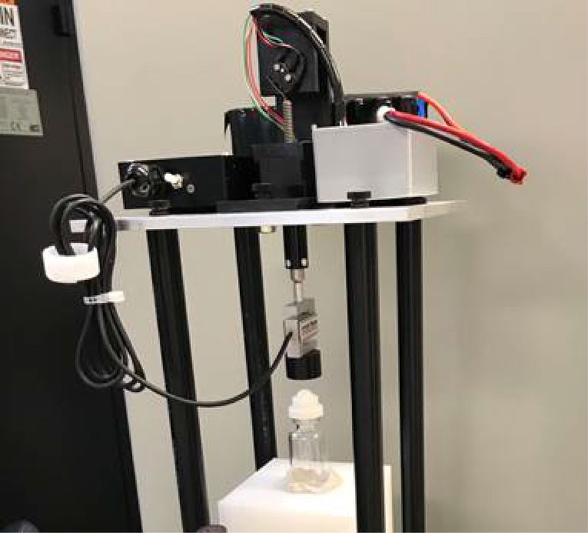
452                                                                                           IEEE TRANSACTIONS ON COMPUTATIONAL IMAGING, VOL. 7, 2021

Fig. 4. Architecture of our 2.5D CNN denoiser. Different sizes of input and
output necessitate a selection operator for the residual connection. Each green
rectangle denotes a tensor, and each ellipse denotes an operation. Blue ellipses
specify the shape of the convolution kernel.

                                                                                   Fig. 6. Illustration of distributed computation of multi-slice fusion. We per-
                                                                                   form distributed computation of the F operator which is the main computational
                                                                                   bottleneck in Algorithm III. Each operator within F , namely Hxy,t , Hyz,t , Hzx,t ,
                                                                                   and L can be executed in parallel. Furthermore, operators Hxy,t , Hyz,t , Hzx,t , and
                                                                                   L are 3D operators that can process the 4D volume “slice by slice” leading to
                                                                                   a large number of concurrent operations that can be distributed among multiple
                                                                                   compute nodes.

                                                                                   input information from a third dimension. The channel dimen-
                                                                                   sion of a convolution layer is typically used to input multiple
                                                                                   color channels for denoising 2D color images using CNNs. We
                                                                                   re-purpose the channel dimension to input five adjacent 2D slices
Fig. 5. Illustration of our training data generation. We extract 3D patches from   of the noisy image to the network and output the denoised center
a typical CT volume and add additive white Gaussian noise (AWGN) to generate       slice. The other slices are being denoised by shifting the 5-slice
training pairs. This makes the training process self-supervised.
                                                                                   moving window. We call this 2.5D since the receptive field along
                             TABLE I                                               the convolution dimensions is large but in the channel dimension
      TOTAL RECONSTRUCTION TIME OF MULTI-SLICE FUSION FOR EACH                     is small. It has been shown that this type of 2.5D processing
                        EXPERIMENTAL CASE                                          is a computationally efficient way of performing effective 3D
                                                                                   denoising with CNNs [7], [20]. We use the notation Hxy,t to
                                                                                   denote a CNN space-time denoiser that performs convolution in
                                                                                   the xy-plane and uses the convolution channels to input slices
                                                                                   from neighboring time-points. The denoisers Hyz,t and Hzx,t are
                                                                                   analogous to Hxy,t but are applied along the yz and zx-plane,
                                                                                   respectively. This orientation of the three denoisers ensures that
                                                                                      1) The spatial dimensions x, y, z are treated equivalently. This
F encompassing all four agents can be written as                                          ensures the regularization to be uniform across all spatial
                                                                                          dimensions;
                           ⎡             ⎤
                               L(W0 )                                                 2) Each dimension in x, y, z, and t is considered at least once.
                           ⎢             ⎥                                                This ensures that model fusion using MACE incorporates
                           ⎢             ⎥
                           ⎢Hxy,t (W1 )⎥                                                  information along all four dimensions.
                           ⎢             ⎥
                 F (W ) = ⎢              ⎥ .                              (14)        Since the three denoising operators Hxy,t , Hyz,t , and Hzx,t pro-
                           ⎢             ⎥
                           ⎢Hyz,t (W2 )⎥                                           cess the 4D volume “slice by slice,” they can be implemented in
                           ⎢             ⎥
                           ⎣             ⎦                                         parallel on large scale parallel computers. Details on distributed
                             Hzx,t (W3 )                                           implementation are described in Section VI.

Here the representative variable W ∈ R4˜N is formed by stack-
                                                                                                      V. TRAINING OF CNN DENOISERS
ing four vectorized 4D volumes.
   The three denoisers Hxy,t , Hyz,t , and Hzx,t share the same                       All three prior model agents Hxy,t , Hyz,t , and Hzx,t in multi-
architecture and trained model but are applied along different                     slice fusion share the same 2.5D model shown in Fig. 4 but are
planes of the 4D space. The CNN architecture is shown in                           oriented along different planes. Consequently we train a single
Fig. 4. We have modified a typical CNN architecture [29] to                        2.5D CNN model using 3D data. Even though the CNN needs

            Authorized licensed use limited to: Purdue University. Downloaded on May 20,2021 at 16:36:28 UTC from IEEE Xplore. Restrictions apply.
MAJEE et al.: MULTI-SLICE FUSION FOR SPARSE-VIEW AND LIMITED-ANGLE 4D CT RECONSTRUCTION                                                                    453

Fig. 7. Comparison of different methods for simulated data 360◦ . Each image is a slice through the reconstructed object for one time-point along the spatial
xy-plane. The reconstruction using FBP suffers from high noise and fails to recover the small hole in the bottom of the image. MBIR+TV and MBIR+4D-MRF
suffer from jagged edges and fail to recover the small hole in the bottom of the image. MBIR+Hyz,t and MBIR+Hzx,t suffer from horizontal and vertical streaks,
respectively, since the denoisers were applied in those planes. MBIR+Hxy,t cannot reconstruct the small hole in the bottom of the image since the xy-plane does
not contain sufficient information.

                             TABLE II                                            map in equation 5 and follows from the theory of Plug-and-
        EXPERIMENTAL SPECIFICATIONS FOR SIMULATED DATA 360◦
                                                                                 play [13], [14].

                                                                                                 VI. DISTRIBUTED RECONSTRUCTION
                                                                                    The computational structure of multi-slice fusion is well-
                                                                                 suited to a highly distributed implementation. The main com-
                            TABLE III                                            putational bottleneck in Algorithm III is the F operator. Fortu-
   QUANTITATIVE EVALUATION FOR SIMULATED DATA 360◦ . MULTI-SLICE                 nately, F is a parallel operator and thus its individual compo-
   FUSION HAS THE HIGHEST PSNR AND SSIM METRIC AMONG ALL THE
                            METHODS                                              nents L, Hxy,t , Hyz,t , and Hzx,t can be executed in parallel. The
                                                                                 operators L, Hxy,t , Hyz,t , and Hzx,t can themselves be parallelized
                                                                                 internally as well. The distributed implementation of multi-slice
                                                                                 fusion is illustrated in Fig. 6.
                                                                                    The CNN denoisers Hxy,t , Hyz,t , and Hzx,t are 2.5D denoisers
                                                                                 that denoise the 4D volume by processing it slice by slice and
                                                                                 thus can be trivially parallelized leading to a large number of
                                                                                 concurrent operations. The concurrent operations for all three
                                                                                 denoisers are distributed among multiple GPUs due to the
                                                                                 availability of optimized GPU routines in Tensorflow. In our
                                                                                 experiments we used a GPU cluster with three Nvidia Tesla
to denoise 3D time-space data, we train it using 3D spatial data                 P100 GPUs to compute the CNN denoising operators.
since 3D volumes are widely available unlike time-space data.                       The cone-beam inversion operator, L, can also be computed
   Fig. 5 outlines our training data generation. We start with a                 for each time-point independently due to the separable structure
low-noise 3D CT volume that is representative of the objects to                  in equations (4) and (2). This leads to a large number of con-
be reconstructed. We extract 3D patches from the CT volume                       current operations which are distributed among multiple CPU
and add pseudo-random additive white Gaussian noise (AWGN)                       nodes. The cone-beam inversion for each time-point is computed
to the patches to generate the training pairs. We then train the                 using a coordinate-descent minimization with multi-threaded
CNN to remove the noise. The use of AWGN is due to the                           parallelism. Further details about the cone-beam inversion can
mathematical form of the quadratic norm term in the proximal                     be found in [3].

             Authorized licensed use limited to: Purdue University. Downloaded on May 20,2021 at 16:36:28 UTC from IEEE Xplore. Restrictions apply.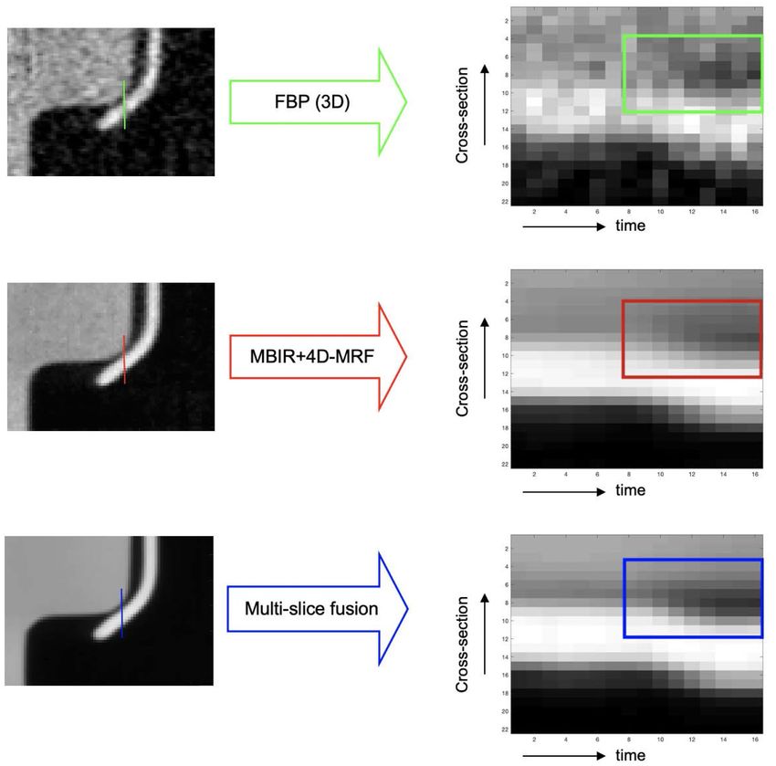
454                                                                                          IEEE TRANSACTIONS ON COMPUTATIONAL IMAGING, VOL. 7, 2021

                                                                                                                 TABLE VI
                                                                                     EXPERIMENTAL SPECIFICATIONS FOR REAL DATA 360◦ : VIAL COMPRESSION

                                                                                       2) Simulated Data 90◦ : Sparse-view limited-angle results
                                                                                           on simulated data with a set of sparse views ranging over
                                                                                           90◦ at each reconstructed time-point;
                                                                                       3) Real Data 360◦ : Sparse-view results on real data with a
                                                                                           set of sparse views ranging over 360◦ at each reconstructed
                                                                                           time-point;
                                                                                       4) Real Data 90◦ : Sparse-view limited-angle results on real
                                                                                           data with a set of sparse views ranging over 90◦ at each
                                                                                           reconstructed time-point.
                                                                                       The selection of the rotation range per time-point is arbitrary
Fig. 8. Plot of cross-section through the phantom and reconstructions from          and can be chosen after the measurements have been taken.
simulated data 360◦ . Multi-slice fusion results in the most accurate reconstruc-   For example, a full rotation with 400 views can be used as a
tion of the gap between materials.
                                                                                    single time-point or as four time-points with 100 views each.
                                                                                    The four time-points per rotation can provide extra temporal
                              TABLE IV                                              resolution, however, they require a more difficult reconstruction
          EXPERIMENTAL SPECIFICATIONS FOR SIMULATED DATA 90◦
                                                                                    with incomplete information.
                                                                                       We compare multi-slice fusion with several other methods
                                                                                    outlined below
                                                                                        r FBP: Conventional 3D filtered back projection reconstruc-
                                                                                          tion;
                                                                                        r MBIR+TV: MBIR reconstruction using a total variation
                                                                                          (TV) prior [30] in the spatial dimensions;
                                                                                        r MBIR+4D-MRF: MBIR reconstruction using 4D Markov
                            TABLE V                                                       random field prior [2] with q = 2.2, p = 1.1, 26 spatial
QUANTITATIVE EVALUATION FOR SIMULATED DATA 90◦ . MULTI-SLICE FUSION                       neighbors and 2 temporal neighbors;
 HAS THE HIGHEST PSNR AND SSIM METRIC AMONG ALL THE METHODS                             r MBIR+Hxy,t : MBIR using the CNN Hxy,t as a PnP prior;
                                                                                        r MBIR+Hyz,t : MBIR using the CNN Hyz,t as a PnP prior;
                                                                                        r MBIR+Hzx,t : MBIR using the CNN Hzx,t as a PnP prior.
                                                                                       We used two CPU cluster nodes, each with 20 Kaby Lake
                                                                                    CPU cores and 96 GB system memory to compute the cone-
                                                                                    beam inversion. We used three GPU nodes, each with a Nvidia
                                                                                    Tesla P100 GPU (16 GB GPU-memory) and 192 GB system
                                                                                    memory to compute the CNN denoisers. To compute the multi-
                                                                                    slice fusion reconstruction, we run Algorithm III for 10 Mann
                    VII. EXPERIMENTAL RESULTS
                                                                                    iterations, with 3 iterations of cone-beam inversion per Mann
   We present experimental results on two simulated and two                         iteration. The total reconstruction time of multi-slice fusion for
real 4D X-ray CT data for Non-Destructive Evaluation (NDE)                          each experimental case are given in Table I.
applications to demonstrate the improved reconstruction quality                        The 2.5D CNN denoiser model used in the reconstructions
of our method. The four experimental cases are outlined below                       was trained using a low-noise 3D CT reconstruction of a bottle
   1) Simulated Data 360◦ : Sparse-view results on simulated                        and screw cap made from different plastics. The object is rep-
      data with a set of sparse views ranging over 360◦ at each                     resentative of a variety of Non-Destructive Evaluation (NDE)
      reconstructed time-point;                                                     problems in which the objects to be imaged are constructed

            Authorized licensed use limited to: Purdue University. Downloaded on May 20,2021 at 16:36:28 UTC from IEEE Xplore. Restrictions apply.
MAJEE et al.: MULTI-SLICE FUSION FOR SPARSE-VIEW AND LIMITED-ANGLE 4D CT RECONSTRUCTION                                                                                455

Fig. 9. Comparison of different methods for simulated data with 90◦ rotation of object per time-point. The FBP reconstruction has severe limited-angle artifacts.
MBIR+TV improves the reconstruction in some regions but it suffers in areas affected by limited angular information. MBIR+4D-MRF reduces limited-angle
artifacts, but allows severe artifacts to form that are not necessarily consistent with real 4D image sequences. In contrast, the multi-slice fusion result does not suffer
from major limited-angle artifacts.

              Authorized licensed use limited to: Purdue University. Downloaded on May 20,2021 at 16:36:28 UTC from IEEE Xplore. Restrictions apply.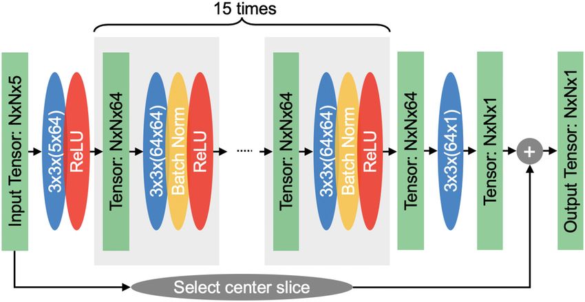
456 IEEE TRANSACTIONS ON COMPUTATIONAL IMAGING, VOL. 7, 2021
TABLE VII
EXPERIMENTAL SPECIFICATIONS FOR REAL DATA 90◦ : INJECTOR PEN
is reconstructed from a sparse set of views spanning 360◦ . We
take a low-noise CT reconstruction of a bottle and screw cap
and denoise it further using BM4D [18] to generate a clean
3D volume to be used as a 3D phantom. We then vertically
translate the 3D phantom by one pixel per time-point to
generate a 4D phantom x0 . We generate simulated sinogram
measurements as N (Ax0 , Λ−1 ) where A is the projection matrix
and the inverse covariance matrix Λ = diag{c exp{−Ax0 }
accounts for the non-uniform noise variance due to a Gaussian
approximation [23] of the underlying Poisson noise. We then
perform a 4D reconstruction from the simulated sinogram
data and compare with the 4D phantom. The experimental
specifications are summarized in Table II.
Fig. 7 compares reconstructions using multi-slice fusion with
several other methods. Each image is a slice through the recon-
structed object for one time-point along the spatial xy-plane.
The reconstruction using FBP suffers from high noise and fails
to recover the small hole in the bottom of the image. The
reconstructions using MBIR+TV and MBIR+4D-MRF suffer
from jagged edges and fail to recover the small hole in the
bottom of the image. MBIR+Hyz,t and MBIR+Hzx,t suffer from
horizontal and vertical streaks, respectively, since the denoisers
were applied in those planes. MBIR+Hxy,t does not suffer from
streaks in the figure since we are viewing a slice along the
xy-plane, but it suffers from other artifacts. MBIR+Hxy,t cannot
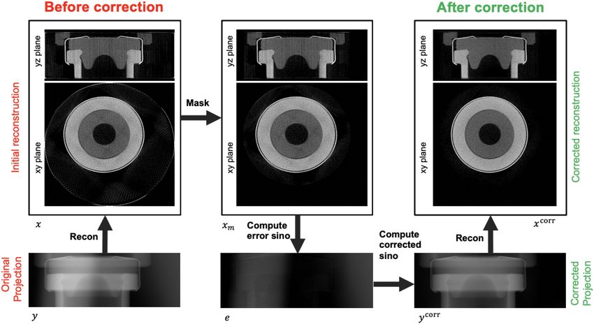
Fig. 10. Illustration of the reconstruction quality obtained for extreme sparse- reconstruct the small hole in the bottom of the image since the
view data with different levels of limited angle per time-point. FBP results xy-plane does not contain sufficient information. It is to be noted
in strong artifacts due to sparse-views and limited angles. MBIR+TV and
MBIR+4D-MRF mitigates most of the major sparse-view artifacts but suffers that multi-slice fusion enhances the size and contrast of the small
from limited angle artifacts in the 90◦ limited angle case. Multi-slice fusion hole highlighted by the blue circle relative to the phantom. This
results in fewer limited-angle and sparse-view artifacts and an improved PSNR can cause deviations when measuring the size of small features
metric. Moreover, multi-slice fusion results in reduced artifacts compared to
MBIR+TV and MBIR+4D-MRF as the rotation per time point is decreased. in the reconstruction.
Next we plot a cross-section through the object for multi-slice
fusion, MBIR+4D-MRF, MBIR+TV, FBP, and the phantom in
from a relatively small number of distinct materials. The ex- Fig. 8. Multi-slice fusion results in the most accurate reconstruc-
tracted patches were normalized to [0,1] and random rotation, tion of the gap between materials.
mirroring, intensity shift were applied. The standard deviation Finally we report the peak signal to noise ratio (PSNR) and the
of the additive white Gaussian noise added during training was structural similarity index measure (SSIM) [31] with respect to
0.1. the phantom for each method in Table III to objectively measure
image quality. We define the PSNR for a given 4D reconstruction
x with a phantom x0 as
A. Simulated Data 360◦
In this section we present results on simulated data to Range(x0 )
PSNR(x) = 20 log10 , (15)
evaluate our method in a sparse-view setting. Each time-point RMSE(x, x0 )
Authorized licensed use limited to: Purdue University. Downloaded on May 20,2021 at 16:36:28 UTC from IEEE Xplore. Restrictions apply.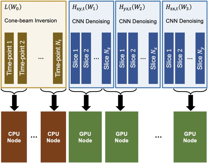
MAJEE et al.: MULTI-SLICE FUSION FOR SPARSE-VIEW AND LIMITED-ANGLE 4D CT RECONSTRUCTION                                                                            457

Fig. 11. Comparison of different methods for Real Data 360◦ : vial. Each image is a slice through the reconstructed vial for one time-point along the spatial xy-plane.
Both FBP and MBIR+4D-MRF suffer from obvious windmill artifacts, higher noise and blurred edges. In contrast to that, the multi-slice fusion reconstruction
has smooth and uniform textures while preserving edge definition. MBIR+Hyz,t and MBIR+Hzx,t suffer from horizontal and vertical streaks. MBIR+Hxy,t cannot
reconstruct the outer ring since the slice displayed is at the edge of the aluminum seal and the xy-plane does not contain sufficient information. Multi-slice fusion
can resolve the edges of the rings better than either of MBIR+Hxy,t , MBIR+Hyz,t , and MBIR+Hzx,t since it has information from all the spatial coordinates.

where range is computed from the 0.1st and 99.9th percentiles of                     90◦ . The simulated measurement data is generated in a similar
the phantom. As can be seen from Table III, multi-slice fusion                       fashion as Section VII-A using the experimental specifications
results in the highest PSNR and SSIM scores.                                         summarized in Table IV.
                                                                                        Fig. 9 shows a comparison of different methods for simu-
                                                                                     lated data with 90◦ rotation of object per time-point. The FBP
B. Simulated Data 90◦                                                                reconstruction has severe limited-angle artifacts. MBIR+TV
   In this section we present results on simulated data to evaluate                  improves the reconstruction in some regions but it suffers in
our method in a sparse-view and limited-angle setting. Each                          areas affected by limited angular information. MBIR+4D-MRF
time-point is reconstructed from a sparse set of views spanning                      reduces limited-angle artifacts, but allows severe artifacts to

             Authorized licensed use limited to: Purdue University. Downloaded on May 20,2021 at 16:36:28 UTC from IEEE Xplore. Restrictions apply.
458 IEEE TRANSACTIONS ON COMPUTATIONAL IMAGING, VOL. 7, 2021
form that are not necessarily consistent with real 4D image
sequences. In contrast, the multi-slice fusion result does not
suffer from major limited-angle artifacts.
Table V shows peak signal to noise ratio (PSNR) and structural
similarity index measure (SSIM) with respect to the phantom for
each method. Multi-slice fusion results in the highest PSNR and
SSIM scores.
In order to determine the effectiveness of our method for more
challenging data, we generate extreme sparse-view simulated
data with different angle of rotation per time-point while keeping
the rest of the experimental setup the same as Table IV. Fig. 10
illustrates the reconstruction quality obtained for the extreme
sparse-view data with different levels of limited angle. FBP
results in strong artifacts due to sparse-views and limited angles.
MBIR+TV and MBIR+4D-MRF mitigates most of the major
sparse-view artifacts but suffers from limited angle artifacts in
the 90◦ limited angle case. Multi-slice fusion results in fewer
limited-angle and sparse-view artifacts and an improved PSNR
metric. Moreover, multi-slice fusion results in a reduced mo-
tion and sparse view artifacts as compared to MBIR+TV and
MBIR+4D-MRF as the rotation per time point is decreased.
C. Real Data 360◦ : Vial Compression
In this section we present results on real data to evaluate our
method in a sparse-view setting. The data is from a dynamic
cone-beam X-ray scan of a glass vial, with elastomeric stopper
and aluminum crimp-seal, using a North Star Imaging X50 X-ray
CT system. The experimental specifications are summarized in Fig. 12. Plot of cross-section through the vial at a time when the aluminum
Table VI. and glass have physically separated. Multi-slice fusion is able to resolve the
junction between materials better while simultaneously producing a smoother
The vial is undergoing dynamic compression during the scan, reconstruction within materials compared to MBIR+4D-MRF and FBP.
to capture the mechanical response of the components as shown
in Fig. 15. Of particular interest is the moment when the alu-
minum seal is no longer in contact with the underside of the
glass neck finish. This indicates the moment when the force
applied exceeds that exerted by the rubber on the glass; this is
known as the “residual seal force” [32].
During the scan, the vial was held in place by fixtures that
were placed out of the field of view as shown in Fig. 15. As
the object rotated, the fixtures periodically intercepted the path
of the X-rays resulting in corrupted measurements and conse-
quently artifacts in the reconstruction. To mitigate this prob-
lem, we incorporate additional corrections that are described in
Appendix A.
Fig. 11 compares multi-slice fusion with several other meth-
ods. Each image is a slice through the reconstructed vial for one
time-point along the spatial xy-plane. Both FBP and MBIR+4D-
MRF suffer from obvious artifacts, higher noise and blurred
edges. In contrast to that, the multi-slice fusion reconstruction
has smooth and uniform textures while preserving edge def-
inition. Fig. 11 also illustrates the effect of model fusion by
comparing multi-slice fusion with MBIR+Hxy,t , MBIR+Hyz,t ,
and MBIR+Hzx,t . MBIR+Hyz,t and MBIR+Hzx,t suffer from
horizontal and vertical streaks respectively since the denoisers Fig. 13. Illustration of temporal resolution for real data 360◦ : vial. We
plot a cross-section through the vial with time for each method: multi-slice
were applied in those planes. MBIR+Hxy,t does not suffer from fusion, MBIR+4D-MRF, FBP. Multi-slice fusion results in improved space-time
streaks in the figure since we are viewing a slice along the resolution of the separation of aluminum and glass.
Authorized licensed use limited to: Purdue University. Downloaded on May 20,2021 at 16:36:28 UTC from IEEE Xplore. Restrictions apply.MAJEE et al.: MULTI-SLICE FUSION FOR SPARSE-VIEW AND LIMITED-ANGLE 4D CT RECONSTRUCTION 459
Fig. 14. Volume rendering of the reconstructed spring and its cross-section for four time-points. A 90◦ limited set of views is used to reconstruct each time-point.
The FBP reconstruction contains severe limited-angle artifacts. MBIR+4D-MRF mitigates some limited-angle artifacts but some artifacts remain.
Next, we plot a cross-section through the object for multi-
slice fusion, MBIR+4D-MRF and FBP in Fig. 12. For this, we
choose a time-point where we know the aluminum and glass
have separated spatially, thus creating an air-gap. Multi-slice
fusion results in a deeper and more defined reconstruction of
the gap between materials. This supports that multi-slice fusion
is able to preserve fine details in spite of producing a smooth
regularized image.
Finally in Fig. 13 we plot a cross-section through the object
with respect to time to show the improved space-time resolution
of our method. We do this for FBP, MBIR+4D-MRF and multi-
slice fusion. Multi-slice fusion results in improved space-time
resolution of the separation of aluminum and glass.
D. Real Data 90◦ : Injector Pen
Fig. 15. Experimental setup for Real Data 360◦ : Vial Compression. The vial
is undergoing dynamic compression during the scan, to capture the mechanical In this section we present results on real data to evaluate our
response of the components. The glass vial (center) and the actuator (top) method in a sparse-view and limited-angle setting. The data is
are held together by a frame constructed of tubes and plates. The tubes were from a dynamic cone-beam X-ray scan of an injector pen using
placed outside the field of view of the CT scanner, thus causing artifacts in the
reconstruction. We describe a correction for this in Appendix X. a North Star Imaging X50 X-ray CT system. The experimental
specifications are summarized in Table VII.
The injection device is initiated before the dynamic scan
starts and completes a full injection during the duration of the
xy-plane, but it suffers from other artifacts. MBIR+Hxy,t cannot scan. We are interested in observing the motion of a particular
reconstruct the outer ring since the slice displayed is at the edge spring within the injector pen in order to determine whether it
of the aluminum seal and the xy-plane does not contain sufficient is working as expected. The spring in question is a non-helical
information. In contrast, multi-slice fusion can resolve the edges wave-spring [33] that is constructed out of circular rings that are
of the rings better than either of MBIR+Hxy,t , MBIR+Hyz,t , joined together. The spring exhibits a fast motion and as a result
and MBIR+Hzx,t since it uses information from all the spatial we need a high temporal resolution to observe the motion of the
coordinates. spring. To have sufficient temporal resolution we reconstruct
Authorized licensed use limited to: Purdue University. Downloaded on May 20,2021 at 16:36:28 UTC from IEEE Xplore. Restrictions apply.460 IEEE TRANSACTIONS ON COMPUTATIONAL IMAGING, VOL. 7, 2021
Fig. 16. Pipeline of the blind fixture correction in Algorithm 2. The vertical stripes in the yz-plane of the reconstruction and the ring at the edge of the field of
view in the xy-plane of the reconstruction have been rectified after performing the correction.
one frame for every 90◦ rotation of the object instead of the
Algorithm 2: Blind fixture correction.
conventional 360◦ rotation.
Input:Original Sinogram: y
Fig. 14 shows a volume rendering of the reconstructed spring
System Matrix: A,
and a cross-section through it for four time-points and re-
Output:Corrected Sinogram: y corr
construction methods FBP, MBIR+4D-MRF, and multi-slice
1 x ← recon(y, A)
fusion. The FBP reconstruction contains severe limited-angle
2 xm ← mask(x)
artifacts. MBIR+4D-MRF mitigates some limited-angle arti-
3 e ← y − Axm
facts but some artifacts remain. In contrast, multi-slice fusion
4 p ← blur(e)
mitigates most limited-angle artifacts. The cross-sections of
5 c ← arg minc∈R e − cp2
the spring in the multi-slice fusion reconstruction are more
6 y corr ← y − cp
circular than the other methods, which align with our prior
knowledge about the spring. The fast compression of the spring
causes the rings within the spring to move significantly within
a time-point, resulting in the observed blur in the multi-slice
fusion reconstruction. Strong limited-angle artifacts in the other together by a fixture constructed of tubes and plates. The tubes
reconstructions mask this effect. were placed outside the field of view of the CT scanner, thus
causing artifacts in the reconstruction. Our method performs
a blind source separation of the projection of the object from
VIII. CONCLUSION
that of the tubes. Our blind separation relies on the fact that the
In this paper, we proposed a novel 4D X-ray CT reconstruc- projection of the tubes is spatially smooth. This is true since the
tion algorithm, multi-slice fusion, that combines multiple low- tubes themselves do not have sharp features and there is motion
dimensional denoisers to form a 4D prior. Our method allows the blur due to the large distance of the tubes from the rotation axis.
formation of an advanced 4D prior using state-of-the-art CNN Algorithm 2 shows our correction algorithm for the fixtures.
denoisers without needing to train on 4D data. Furthermore, it Fig. 16 illustrates the algorithm pictorially. The initial recon-
allows for multiple levels of parallelism, thus enabling recon- struction x suffers from artifacts within the image and at the
struction of large volumes in a reasonable time. Although we edge of the field of view. We mask x using a cylindrical mask
focused on 4D X-ray CT reconstruction for NDE applications, slightly smaller than the field of view to obtain the masked image
our method can be used for any reconstruction problem involving xm . This is done so that the majority of the artifacts at the edge of
multiple dimensions. the field of view are masked but the object remains unchanged in
xm . Consequently the error sinogram e = y − Axm primarily
IX. APPENDIX contains the projection of the tubes with some residual projection
of the object. The blurring of e filters out the residual object pro-
X. CORRECTION FOR FIXTURES OUTSIDE THE FIELD OF VIEW jection but preserves the spatially smooth projection of the tubes.
Here we describe our correction for fixtures placed out of the The corrected measurements y corr are found after performing a
field of view of the scanner. As shown in Fig. 15, the setup is held least squares fit. The correction can be repeated in order to get
Authorized licensed use limited to: Purdue University. Downloaded on May 20,2021 at 16:36:28 UTC from IEEE Xplore. Restrictions apply.MAJEE et al.: MULTI-SLICE FUSION FOR SPARSE-VIEW AND LIMITED-ANGLE 4D CT RECONSTRUCTION 461
an improved reconstruction x and consequently an improved [12] D. Clark and C. Badea, “Convolutional regularization methods for 4D,
correction y corr . X-ray CT reconstruction,” Phys. Med. Imag., vol. 10948. Int. Soc. Opt.
Photon., 2019, Art no. 109482A.
Fig. 16 shows the sinogram and reconstruction both before [13] S. Sreehari et al., “Plug-and-play priors for bright field electron tomogra-
and after performing the blind correction. Not only does the phy and sparse interpolation,” IEEE Trans. Comput. Imag., vol. 2, no. 4,
reconstruction after fixture correction remove the artifacts in pp. 408–423, Dec. 2016.
[14] S. V. Venkatakrishnan, C. A. Bouman, and B. Wohlberg, “Plug-and-play
the air region, but it also improves the image quality inside the priors for model based reconstruction,” in Proc. Glob. Conf. Signal Inf.
object. It can be seen that the vertical stripes in the object in Process., 2013, pp. 945–948.
the yz view of the reconstruction have been eliminated after [15] Y. Sun, B. Wohlberg, and U. S. Kamilov, “An online plug-and-play algo-
rithm for regularized image reconstruction,” IEEETrans. Comput. Imag.,
performing the correction. vol. 5, no. 3, pp. 395–408, 2019.
[16] U. S. Kamilov, H. Mansour, and B. Wohlberg, “A plug-and-play priors
ACKNOWLEDGMENT approach for solving nonlinear imaging inverse problems,” IEEE Signal
Process. Lett., vol. 24, no. 12, pp. 1872–1876, Dec. 2017.
The authors would like to acknowledge support from Eli [17] K. Dabov, A. Foi, V. Katkovnik, and K. Egiazarian, “Image denoising by
sparse 3D transform-domain collaborative filtering,” IEEE Trans. Image
Lilly and Company under research project funding agreement Process., vol. 16, no. 8, pp. 2080–2095, 2007.
17099289. Charles A. Bouman and Gregery T. Buzzard were [18] M. Maggioni, G. Boracchi, A. Foi, and K. Egiazarian, “Video denoising
supported in part by NSF grant CCF-1763896. We also thank M. using separable 4D nonlocal spatiotemporal transforms,” Image Process.:
Algorithms Syst. IX, vol. 7870. Int. Soc. Opt. Photon., 2011, p. 787003.
Cory Victor and Dr. Coralie Richard from Eli Lilly and Company [19] G. T. Buzzard, S. H. Chan, S. Sreehari, and C. A. Bouman, “Plug-
for their assistance and guidance in setting up the residual seal and-play unplugged: Optimization-free reconstruction using consensus
force test experiment. equilibrium,” SIAM J. Imag. Sci., vol. 11, no. 3, pp. 2001–2020, 2018.
[20] D. Jiang, W. Dou, L. Vosters, X. Xu, Y. Sun, and T. Tan, “Denoising
of 3D magnetic resonance images with multi-channel residual learning of
convolutional neural network,” Jpn. J. Radiol., vol. 36, no. 9, pp. 566–574,
REFERENCES 2018.
[21] Y. Sun, B. Wohlberg, and U. S. Kamilov, “Plug-in stochastic gradient
[1] C. Huang, J. L. Ackerman, Y. Petibon, T. J. Brady, G. El Fakhri, and method,” 2018, arXiv:1811.03659.
J. Ouyang, “MR-based motion correction for PET imaging using wired [22] Y. Sun, S. Xu, Y. Li, L. Tian, B. Wohlberg, and U. S. Kamilov, “Regularized
active MR microcoils in simultaneous PET-MR: Phantom study,” Med. fourier ptychography using an online plug-and-play algorithm,” in Proc.
Phys., vol. 41, no. 4, 2014, Art no. 041910. IEEE Int. Conf. Acoust., Speech Signal Process., 2019, pp. 7665–7669.
[2] K. A. Mohan et al., “TIMBIR: A method for time-space reconstruc- [23] C. A. Bouman and K. Sauer, “A unified approach to statistical tomography
tion from interlaced views.” IEEE Trans. Comput. Imag., vol. 1, no. 2, using coordinate descent optimization,” IEEE Trans. Image Process.,
pp. 96–111, Jun. 2015. vol. 5, no. 3, pp. 480–492, Mar. 1996.
[3] T. Balke et al., “Separable models for cone-beam MBIR reconstruction,” [24] V. Sridhar, G. T. Buzzard, and C. A. Bouman, “Distributed framework
Electron. Imag., vol. 2018, no. 15, pp. 181–1, 2018. for fast iterative CT reconstruction from view-subsets,” Electron. Imag.,
[4] S. Majee, T. Balke, C. A. Kemp, G. T. Buzzard, and C. A. Bouman, “4D vol. 2018, no. 15, pp. 102–1, 2018.
X-ray CT reconstruction using multi-slice fusion,” in Proc. IEEE Int. Conf. [25] J.-J. Moreau, “Proximité et dualité dans un espace hilbertien,” Bull. de la
Comput. Photogr., 2019, pp. 1–8. Société Mathématique de France, vol. 93, pp. 273–299, 1965.
[5] Z. Nadir, M. S. Brown, M. L. Comer, and C. A. Bouman, “A model- [26] R. E. Williamson, R. H. Crowell, and H. F. Trotter, Calculus of Vector
based iterative reconstruction approach to tunable diode laser absorption Functions. Englewood Cliffs, NJ, USA: Prentice-Hall, 1972.
tomography,” IEEE Trans. Comput. Imag., vol. 3, no. 4, pp. 876–890, [27] V. Sridhar, X. Wang, G. T. Buzzard, and C. A. Bouman, “Distributed
Dec. 2017. memory framework for fast iterative CT reconstruction from view-subsets
[6] S. Majee, D. H. Ye, G. T. Buzzard, and C. A. Bouman, “A model based using multi-agent consensus equilibrium,” Manuscript Preparation IEEE
neuron detection approach using sparse location priors,” Electron. Imag., Trans. Comput. Imag., 2018.
vol. 2017, no. 17, pp. 10–17, 2017. [28] S. Boyd et al., “Distributed optimization and statistical learning via the
[7] A. Ziabari, D. H. Ye, K. D. Sauer, J. Thibault, and C. A. Bouman, alternating direction method of multipliers,” Found. Trends Mach. Learn.,
“2.5D deep learning for CT image reconstruction using a multi-GPU vol. 3, no. 1, pp. 1–122, 2011.
implementation,” in Proc. 52nd Asilomar Conf. Signals, Syst., Comput., [29] K. Zhang, W. Zuo, Y. Chen, D. Meng, and L. Zhang, “Beyond a Gaussian
2018, pp. 2044–2049. denoiser: Residual learning of deep CNN for image denoising,” IEEE
[8] J. Gibbs et al., “The three-dimensional morphology of growing dendrites,” Trans. Image Process., vol. 26, no. 7, pp. 3142–3155, Jul. 2017.
Sci. Rep., vol. 5, 2015, Art no. 11824. [30] P. Getreuer, “Rudin-osher-fatemi total variation denoising using split
[9] G. Zang, R. Idoughi, R. Tao, G. Lubineau, P. Wonka, and W. Hei- bregman,” Image Process. OnLine, vol. 2, pp. 74–95, 2012.
drich, “Space-time tomography for continuously deforming objects,” ACM [31] Z. Wang, A. C. Bovik, H. R. Sheikh, and E. P. Simoncelli, “Image quality
Trans. Graph., vol. 37, no. 4, pp. 1–14, 2018. assessment: From error visibility to structural similarity,” IEEE Trans.
[10] S. J. Kisner, E. Haneda, C. A. Bouman, S. Skatter, M. Kourinny, and S. Image Process., vol. 13, no. 4, pp. 600–612, Apr. 2004.
Bedford, “Model-based CT reconstruction from sparse views,” in Proc. [32] R. Mathaes et al., “The pharmaceutical vial capping process: Container
2nd Int. Conf. Image Formation X-Ray Computed Tomogr., 2012, pp. 444– closure systems, capping equipment, regulatory framework, and seal qual-
447. ity tests,” Eur. J. Pharmaceutics Biopharmaceutics, vol. 99, pp. 54–64,
[11] K. Sauer and C. Bouman, “A local update strategy for iterative recon- 2016.
struction from projections,” IEEE Trans. Signal Process., vol. 41, no. 2, [33] S. Komura and H. Toyofuku, “Wave spring,” Apr. 22 1997, US
pp. 534–548, 1993. Pat. 5,622, 358.
Authorized licensed use limited to: Purdue University. Downloaded on May 20,2021 at 16:36:28 UTC from IEEE Xplore. Restrictions apply.You can also read