Münchmeyer, J., Bindi, D., Leser, U., Tilmann, F. (2021): Earthquake magnitude and location estimation from real time seismic waveforms with a ...
←
→
Page content transcription
If your browser does not render page correctly, please read the page content below
Münchmeyer, J., Bindi, D., Leser, U., Tilmann, F.
(2021): Earthquake magnitude and location
estimation from real time seismic waveforms with
a transformer network. - Geophysical Journal
International, 226, 2, 1086-1104.

https://doi.org/10.1093/gji/ggab139

Institional Repository GFZpublic: https://gfzpublic.gfz-potsdam.de/

Geophys. J. Int. (2021) 226, 1086–1104                                                                                         doi: 10.1093/gji/ggab139
Advance Access publication 2021 April 12
GJI Seismology

Earthquake magnitude and location estimation from real time
seismic waveforms with a transformer network

                                                                                                                                                           Downloaded from https://academic.oup.com/gji/article/226/2/1086/6223459 by Bibliothek des Wissenschaftsparks Albert Einstein user on 14 June 2021
Jannes Münchmeyer ,1,2 Dino Bindi ,1 Ulf Leser                                          2
                                                                                             and Frederik Tilmann                  1,3
1 Deutsches    GeoForschungsZentrum GFZ, 14473 Potsdam, Germany. E-mail: munchmej@gfz-potsdam.de
2 Institut für Informatik, Humboldt-Universität zu Berlin, 10117 Berlin, Germany
3 Institut für geologische Wissenschaften, Freie Universität Berlin, 14195 Berlin, Germany

Accepted 2021 March 25. Received 2021 March 10; in original form 2021 January 6

                                       SUMMARY
                                       Precise real time estimates of earthquake magnitude and location are essential for early warning
                                       and rapid response. While recently multiple deep learning approaches for fast assessment of
                                       earthquakes have been proposed, they usually rely on either seismic records from a single
                                       station or from a fixed set of seismic stations. Here we introduce a new model for real-
                                       time magnitude and location estimation using the attention based transformer networks. Our
                                       approach incorporates waveforms from a dynamically varying set of stations and outperforms
                                       deep learning baselines in both magnitude and location estimation performance. Furthermore,
                                       it outperforms a classical magnitude estimation algorithm considerably and shows promising
                                       performance in comparison to a classical localization algorithm. Our model is applicable
                                       to real-time prediction and provides realistic uncertainty estimates based on probabilistic
                                       inference. In this work, we furthermore conduct a comprehensive study of the requirements
                                       on training data, the training procedures and the typical failure modes. Using three diverse
                                       and large scale data sets, we conduct targeted experiments and a qualitative error analysis.
                                       Our analysis gives several key insights. First, we can precisely pinpoint the effect of large
                                       training data; for example, a four times larger training set reduces average errors for both
                                       magnitude and location prediction by more than half, and reduces the required time for real
                                       time assessment by a factor of four. Secondly, the basic model systematically underestimates
                                       large magnitude events. This issue can be mitigated, and in some cases completely resolved,
                                       by incorporating events from other regions into the training through transfer learning. Thirdly,
                                       location estimation is highly precise in areas with sufficient training data, but is strongly
                                       degraded for events outside the training distribution, sometimes producing massive outliers.
                                       Our analysis suggests that these characteristics are not only present for our model, but for
                                       most deep learning models for fast assessment published so far. They result from the black
                                       box modeling and their mitigation will likely require imposing physics derived constraints
                                       on the neural network. These characteristics need to be taken into consideration for practical
                                       applications.
                                       Key words: Neural networks, fuzzy logic; Probability distributions; Earthquake early warn-
                                       ing.

                                                                                the raw input data. This property allows the models to use the
1 I N T RO D U C T I O N
                                                                                full information contained in the waveforms of an event. However,
Recently, multiple studies investigated deep learning on raw seismic            the models published so far use fixed time windows and can not
waveforms for the fast assessment of earthquake parameters, such                be applied to data of varying length without retraining. Similarly,
as magnitude (e.g. Lomax et al. 2019; Mousavi & Beroza 2020;                    except the model by van den Ende & Ampuero (2020), all models
van den Ende & Ampuero 2020), location (e.g. Kriegerowski et al.                process either waveforms from only a single seismic station or rely
2019; Mousavi & Beroza 2019; van den Ende & Ampuero 2020)                       on a fixed set of seismic stations defined at training time. The model
and peak ground acceleration (e.g. Jozinović et al. 2020). Deep                by van den Ende & Ampuero (2020) enables the use of a variable
learning is well suited for these tasks, as it does not rely on manually        station set, but combines measurements from multiple stations using
selected features, but can learn to extract relevant information from           a simple pooling mechanism. While it has not been studied so far in

1086
                                               C   The Author(s) 2021. Published by Oxford University Press on behalf of The Royal Astronomical Society.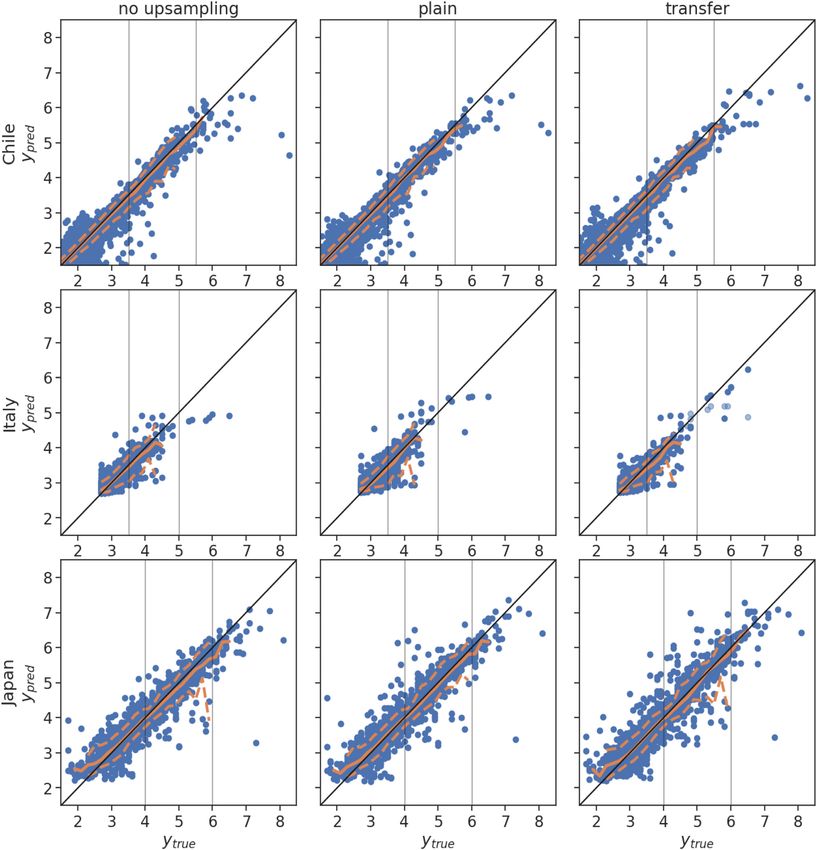
Earthquake assessment with TEAM-LM                  1087

a seismological context, it has been shown in the general domain that      minor changes in the seismic network configuration during the time
set pooling architectures are in practice limited in the complexity        covered by the catalogue, the station set used in the construction of
of functions they can model (Lee et al. 2019).                             this catalogue had been selected to provide a high degree of stability
    Here we introduce a new model for magnitude and location               of the locations accuracy throughout the observational period (Sippl
estimation based on the architecture recently introduced for the           et al. 2018). Similarly, the magnitude scale has been carefully cali-
transformer earthquake alerting model (TEAM, Münchmeyer et al.            brated to achieve a high degree of consistency in spite of significant
2021), a deep learning based earthquake early warning model.               variations of attenuation (Münchmeyer et al. 2020b). This data set
While TEAM estimated PGA at target locations, our model esti-              therefore contains the highest quality labels among the data sets in

                                                                                                                                                      Downloaded from https://academic.oup.com/gji/article/226/2/1086/6223459 by Bibliothek des Wissenschaftsparks Albert Einstein user on 14 June 2021
mates magnitude and hypocentral location of the event. We call             this study. For the Chile data set, we use broad-band seismogramms
our adaptation TEAM-LM, TEAM for location and magnitude es-                from the fixed set of 24 stations used for the creation of the original
timation. We use TEAM as a basis due to its flexible multistation          catalogue and magnitude scale. Although the Chile data set has the
approach and its ability to process incoming data effectively in real-     smallest number of stations of the three data sets, it comprises three
time, issuing updated estimates as additional data become available.       to four times as many waveforms as the other two due to the large
Similar to TEAM, TEAM-LM uses mixture density networks to pro-             number of events.
vided probability distributions rather than merely point estimates as         The data sets for Italy and Japan are more focused on early warn-
predictions. For magnitude estimation, our model outperforms two           ing, containing fewer events and only strong motion waveforms.
state of the art baselines, one using deep learning (van den Ende &        They are based on catalogues from the INGV (ISIDe Working
Ampuero 2020) and one classical approach (Kuyuk & Allen 2013).             Group 2007) and the NIED KiKNet (National Research Institute
For location estimation, our model outperforms a deep learning             For Earth Science And Disaster Resilience 2019), respectively. The
baseline (van den Ende & Ampuero 2020) and shows promising                 data sets each encompass a larger area than the Chile data set and
performance in comparison to a classical localization algorithm.           include waveforms from significantly more stations. In contrast to
    We note a further deficiency of previous studies for deep learning     the Chile data sets, the station coverage differs strongly between
in seismology. Many of these pioneering studies focused their anal-        different events, as only stations recording the event are considered.
ysis on the average performance of the proposed models. Therefore,         In particular, KiKNet stations do not record continuous waveforms,
little is known about the conditions under which these models fail,        but operate in trigger mode, only saving waveforms if an event trig-
the impact of training data characteristics, the possibility of sharing    gered at the station. For Japan each station comprises two sensors,
knowledge across world regions, and of specific training strategies.       one at the surface and one borehole sensor. Therefore for Japan we
All of these are of particular interest when considering practical         have six component recordings (three surface, three borehole) avail-
application of the models.                                                 able instead of the three component recordings for Italy and Chile.
    To address these issues and provide guidance for practitioners, we     A full list of seismic networks used in this study can be found in the
perform a comprehensive evaluation of TEAM-LM on three large               appendix (Table A1).
and diverse data sets: a regional broad-band data set from Northern           For each data set we use the magnitude scale provided in the
Chile, a strong motion data set from Japan and another strong mo-          catalogue. For the Chile catalogue, this is MA , a peak displacement
tion data set from Italy. These data sets differ in their seismotectonic   based scale, but without the Wood-Anderson response and there-
environment (North Chile and Japan: subduction zones; Italy: dom-          fore saturation-free for large events (Münchmeyer et al. 2020b;
inated by both convergent and divergent continental deformation),          Deichmann 2018). For Japan MJMA is used. MJMA combines differ-
their spatial extent (North Chile: regional scale; Italy and Japan: na-    ent magnitude scales, but similarly to MA primarily uses horizontal
tional catalogues), and the instrument type (North Chile: broadband,       peak displacement (Doi 2014). For Italy the catalogue provides dif-
Italy and Japan: strong motion). All three data sets contain hundreds      ferent magnitude types approximately dependent on the size of the
of thousands of waveforms. North Chile is characterized by a rela-         event: ML (>90 per cent of the events), MW (
1088       J. Münchmeyer et al.

                      Table 1. Overview of the data sets. The lower boundary of the magnitude category is the 5th percentile of the
                      magnitude; this limit is chosen as each data set contains a small number of unrepresentative very small events.
                      The upper boundary is the maximum magnitude. Magnitudes are given with two digit precision for Chile, as the
                      precision of the underlying catalogue is higher than for Italy and Japan. The Italy data set uses different magnitudes
                      for different events, which are ML (>90 per cent of the events), MW (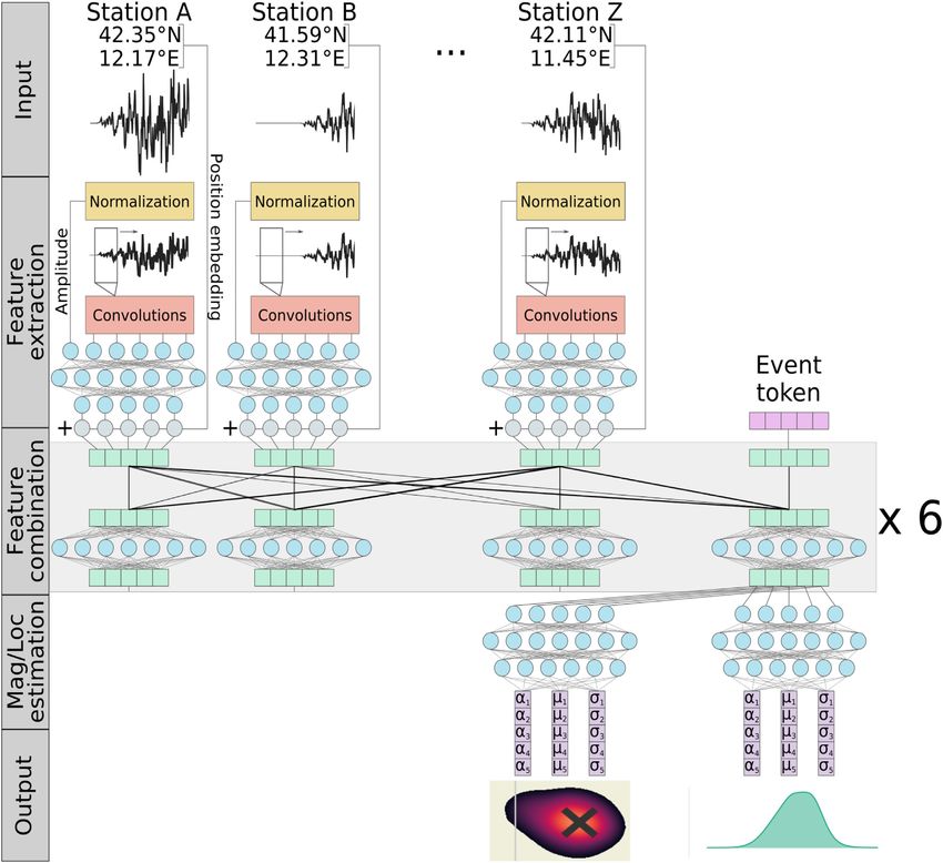
Earthquake assessment with TEAM-LM                       1089

                                                                                                                                                                     Downloaded from https://academic.oup.com/gji/article/226/2/1086/6223459 by Bibliothek des Wissenschaftsparks Albert Einstein user on 14 June 2021
Figure 1. Overview of the data sets. The top row shows the spatial station distribution, the second tow the spatial event distribution. The event depth is encoded
using colour. Higher resolution versions of the maps can be found in the supplementary material (Figs S1, S2 and S3). The bottom row shows the distributions
of the event magnitudes. The magnitude scales are the peak displacement based MA , local magnitude ML , moment magnitude MW , body wave magnitude mb
and MJMA , a magnitude primarily using peak displacement.

et al. 2018). The elements of this event query vector are learned                      The model is trained end-to-end using a log-likelihood loss with
during the training procedure.                                                      the Adam optimizer (Kingma & Ba 2014). We train separate models
   From the transformer output, we only use the output correspond-                  for magnitude and for location. As we observed difficulties in the
ing to the event token, which we term event embedding and which                     onset of the optimization when starting from a fully random initial-
is passed through another multi-layer perceptron predicting the pa-                 ization, we pretrain the feature extraction network. To this end we
rameters and weights of a mixture of Gaussians (Bishop 1994).                       add a mixture density network directly after the feature extraction
We use N = 5 Gaussians for magnitude and N = 15 Gaussians                           and train the resulting network to predict magnitudes from single
for location estimation. For computational and stability reasons,                   station waveforms. We then discard the mixture density network
we constrain the covariance matrix of the individual Gaussians for                  and use the weights of the feature extraction as initialization for
location estimation to a diagonal matrix to reduce the output di-                   the end-to-end training. We use this pretraining method for both
mensionality. Even though uncertainties in latitude, longitude and                  magnitude and localization networks.
depth are known to generally be correlated, this correlation can be                    Similarly to the training procedure for TEAM we make exten-
modeled with diagonal covariance matrices by using the mixture.                     sive use of data augmentation during training. First, we randomly
1090        J. Münchmeyer et al.

                                                                                                                                                                     Downloaded from https://academic.oup.com/gji/article/226/2/1086/6223459 by Bibliothek des Wissenschaftsparks Albert Einstein user on 14 June 2021
Figure 2. Overview of the adapted transformer earthquake alerting model, showing the input, the feature extraction, the feature combination, the magni-
tude/location estimation and the output. For simplicity, not all layers are shown, but only their order and combination is visualized schematically. For the exact
number of layers and the size of each layer please refer to Tables S1 to S3. Please note that the number of input stations is variable, due to the self-attention
mechanism in the feature combination.

select a subset of up to 25 stations from the available station set.                ensuring that the station selection does not introduce a knowledge
We limit the maximum number to 25 for computational reasons.                        leak.
Secondly, we apply temporal blinding, by zeroing waveforms after
a random time t1 . This type of augmentation allows TEAM-LM
to be applied to real time data. We note that this type of temporal                 2.3 Baseline methods
blinding to enable real time predictions would most likely work for
the previously published CNN approaches as well. To avoid knowl-                    Recently, van den Ende & Ampuero (2020) suggested a deep learn-
edge leaks for Italy and Japan, we only use stations as inputs that                 ing method capable of incorporating waveforms from a flexible set
triggered before time t1 for these data sets. This is not necessary for             of stations. Their architecture uses a similar CNN based feature
Chile, as there the maximum number of stations per event is below                   extraction as TEAM-LM. In contrast to TEAM-LM, for feature
25 and waveforms for all events are available for all stations active               combination it uses maximum pooling to aggregate the feature vec-
at that time, irrespective of whether the station actually recorded the             tors from all stations instead of a transformer. In addition they do
event. Thirdly, we oversample large magnitude events, as they are                   not add predefined position embeddings, but concatenate the fea-
strongly underrepresented in the training data set. We discuss the                  ture vector for each station with the location coordinates and apply
effect of this augmentation in further detail in the Results section.               a multilayer perceptron to get the final feature vectors for each sta-
In contrast to the station selection during training, in evaluation                 tion. The model of van den Ende & Ampuero (2020) is both trained
we always use the 25 stations picking first. Again, we only use                     and evaluated on 100 s long waveforms. In its original form it is
stations and their waveforms as input once they triggered, thereby                  therefore not suitable for real time processing, although the real
Earthquake assessment with TEAM-LM                  1091

time processing could be added with the same zero-padding ap-                  TEAM-LM outperforms the classical magnitude baseline con-
proach used for TEAM and TEAM-LM. The detail differences in                 sistently. On two data sets, Chile and Italy, the performance of
the CNN structure and the real-time processing capability make a            TEAM-LM with only 0.5 s of data is superior to the baseline with
comparison of the exact model of van den Ende & Ampuero (2020)              25 s of data. Even on the third data set, Japan, TEAM-LM requires
to TEAM-LM difficult.                                                       only approximately a quarter of the time to reach the same precision
   To still compare TEAM-LM to the techniques introduced in this            as the classical baseline and achieves significantly higher precision
approach, we implemented a model based on the key concepts of               after 25 s. The RMSE for TEAM-LM stabilizes after 16 s for all
van den Ende & Ampuero (2020). As we aim to evaluate the perfor-            data sets with final values of 0.08 m.u. for Chile, 0.20 m.u. for

                                                                                                                                                     Downloaded from https://academic.oup.com/gji/article/226/2/1086/6223459 by Bibliothek des Wissenschaftsparks Albert Einstein user on 14 June 2021
mance differences from the conceptual changes, rather than differ-          Italy and 0.22 m.u. for Japan. The performance differences between
ent hyperparameters, for example the exact size and number of the           TEAM-LM and the classical baseline result from the simplified
convolutional layers, we use the same architecture as TEAM-LM               modelling assumptions for the baseline. While the relationship be-
for the feature extraction and the mixture density output. Addition-        tween early peak displacement and magnitude only holds approx-
ally we train the model for real time processing using zero padding.        imately, TEAM-LM can extract more nuanced features from the
In comparison to TEAM-LM we replace the transformer with a                  waveform. In addition, the relationship for the baseline was origi-
maximum pooling operation and remove the event token.                       nally calibrated for a moment magnitude scale. While all magnitude
   We evaluate two different representations for the position encod-        scales have an approximate 1:1 relationship with moment magni-
ing. In the first, we concatenated the positions to the feature vectors     tude, this might introduce further errors.
as proposed by van den Ende & Ampuero (2020). In the second, we                We further note that the performance of the classical baseline for
add the position embeddings element-wise to the feature vectors as          Italy are consistent with the results reported by Festa et al. (2018).
for TEAM-LM. In both cases, we run a three-layer perceptron over            They analysed early warning performance in a slightly different
the combined feature and position vector for each station, before           setting, looking only at the nine largest events in the 2016 Cen-
applying the pooling operation.                                             tral Italy sequence. However, they report a RMSE of 0.28 m.u. for
   We use the fast magnitude estimation approach (Kuyuk & Allen             the PRESTO system 4 s after the first alert, which matches ap-
2013) as a classical, that is non-deep-learning, baseline for magni-        proximately the 8 s value in our analysis. Similarly, Leyton et al.
tude. The magnitude is estimated from the horizontal peak displace-         (2018) analyse how fast magnitudes can be estimated in subductions
ment in the first seconds of the P wave. As this approach needs to          zones, and obtain values of 0.01 ± 0.28 across all events and −0.70
know the hypocentral distance, it requires knowledge of the event           ± 0.30 for the largest events (MW > 7.5) at 30 s after origin time.
location. We simply provide the method with the catalogue hypocen-          This matches the observed performance of the classical baseline
tre. While this would not be possible in real time, and therefore gives     for Japan. For Chile, our classical baseline performs considerably
the method an unfair advantage over the deep learning approaches,           worse, likely caused by the many small events with bad SNR com-
it allows us to focus on the magnitude estimation capabilities. Fur-        pared to the event set considered by Leyton et al. (2018). However,
thermore, in particular for Italy and Japan, the high station density       TEAM-LM still outperforms the performance numbers reported by
usually allows for sufficiently well constrained location estimates at      Leyton et al. (2018) by a factor of more than 2.
early times. For a full description of this baseline, see supplement           Improvements for TEAM-LM in comparison to the deep learning
section SM 1.                                                               baseline variants are much smaller than to the classical approach.
   As a classical location baseline we use NonLinLoc (Lomax et al.          Still, for the Japan data set at late times, TEAM-LM offers im-
2000) with the 1-D velocity models from Graeber & Asch (1999)               provements of up to 27 per cent for magnitude. For the Italy data
(Chile), Ueno et al. (2002) (Japan) and Matrullo et al. (2013) (Italy).     set, the baseline variants are on par with TEAM-LM. For Chile, only
For the earliest times after the event detection usually only few picks     the baseline with position embeddings is on par with TEAM-LM.
are available. Therefore, we apply two heuristics. Until at least 3/5/5     Notably, for the Italy and Japan data sets, the standard deviation
(Chile/Japan/Italy) picks are available, the epicentre is estimated as      between multiple runs with different random model initialization is
the arithmetic mean of the stations with picked arrivals so far, while      considerably higher for the baselines than for TEAM-LM (Fig. 3,
the depth is set to the median depth in the training data set. Until        error bars). This indicates that the training of TEAM-LM is more
at least 4/7/7 picks are available, we apply NonLinLoc, but fix             stable with regard to model initialization.
the depth to the median depth in the data set. We require higher               The gains of TEAM-LM can be attributed to two differences: the
numbers of picks for Italy and Japan, as the pick quality is lower          transformer for station aggregation and the position embeddings.
than in Chile but the station density is higher. This leads to worse        In our experiments we ruled out further differences, for example
early NonLinLoc estimates in Italy and Japan compared to Chile,             size and structure of the feature extraction CNN, by using identical
but improves the performance of the heuristics.                             network architectures for all parts except the feature combination
                                                                            across stations. Regarding the impact of position embeddings, the
                                                                            results do not show a consistent pattern. Gains for Chile seem to be
                                                                            solely caused by the position embeddings; gains for Italy are gener-
                                                                            ally lowest, but again the model with position embeddings performs
3 R E S U LT S
                                                                            better; for Japan the concatenation model performs slightly better,
                                                                            although the variance in the predictions makes the differences non-
3.1 Magnitude estimation performance
                                                                            significant. We suspect these different patterns to be caused by the
We first compare the estimation capabilities of TEAM-LM to the              different catalogue and network sizes as well as the station spacing.
baselines in terms of magnitude (Fig. 3). We evaluate the models at            We think that gains from using a transformer can be explained
fixed times t = 0.5, 1, 2, 4, 8, 16 and 25 s after the first P arrival at   with its attention mechanism. The attention allows the transformer
any station in the network. In addition to presenting selected results      to focus on specific stations, for example the stations which have
here, we provide tables with the results of further experiments in          recorded the longest waveforms so far. In contrast, the maximum
the supplementary material (Tables S5–S15).                                 pooling operation is less flexible. We suspect that the high gains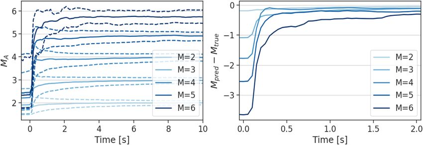
1092        J. Münchmeyer et al.

                                                                                                                                                                     Downloaded from https://academic.oup.com/gji/article/226/2/1086/6223459 by Bibliothek des Wissenschaftsparks Albert Einstein user on 14 June 2021
Figure 3. RMSE of the mean magnitude predictions from TEAM-LM, the pooling model with sinusoidal location embeddings (POOL-E), the pooling model
with concatenated positions (POOL-C) and the classical baseline method. The time indicates the time since the first P arrival at any station, the RMSE is
provided in magnitude units [m.u.]. Error bars indicate ±1 standard deviation when training the model with different random initializations. For better visibility
error bars
       √ are provided with a small x-offset. Standard deviations were obtained from six realizations. Note that the uncertainty of the provided means is by a
factor 6 smaller than the given standard deviation, due to the number of samples. We provide no standard deviation for the baseline, as it does not depend on
a model initialization.

for Japan result from the wide spatial distribution of seismicity                   saturation sets in for large events. Interestingly the saturation starts
and therefore very variable station distribution. While in Italy most               at different magnitudes, which are around 5.5 for Italy and 6.0 for
events are in Central Italy and in Chile the number of stations are                 Chile. For Japan, events up to magnitude 7 are predicted with-
limited, the seismicity in Japan occurs along the whole subduction                  out obvious bias. This saturation behavior is not only visible for
zone with additional onshore events. This complexity can likely be                  TEAM-LM, but has also been observed in prior studies, for ex-
handled better with the flexibility of the transformer than using a                 ample in Mousavi & Beroza (2020, their figs 3, 4). In their work,
pooling operation. This indicates that the gains from using a trans-                with a network trained on significantly smaller events, the saturation
former compared to pooling with position embeddings are likely                      already set in around magnitude 3. The different saturation thresh-
modest for small sets of stations, and highest for large heteroge-                  olds indicate that the primary cause for saturation is not the longer
neous networks.                                                                     rupture duration of large events or other inherent event properties,
   In many use cases, the performance of magnitude estimation al-                   as in cause (ii), but is instead likely related to the low number of
gorithms for large magnitude events is of particular importance. In                 training examples for large events, rendering it nearly impossible
Fig. 4, we compare the RMSE of TEAM-LM and the classical base-                      to learn their general characteristics, as in cause (i). This explana-
lines binned by catalogue magnitude into small, medium and large                    tion is consistent with the much higher saturation threshold for the
events. For Chile/Italy/Japan we count events as small if their mag-                Japanese data set, where the training data set contains a comparably
nitude is below 3.5/3.5/4 and as large if their magnitude is at least               large number of large events, encompassing the year 2011 with the
5.5/5/6. We observe a clear dependence on the event magnitude. For                  Tohoku event and its aftershocks.
all data sets the RMSE for large events is higher than for intermedi-                  As a further check of cause (i), we trained models without up-
ate sized events, which is again higher than for small events. On the               sampling large magnitude events during training, thereby reducing
other hand the decrease in RMSE over time is strongest for larger                   the occurrence of large magnitude events to the natural distribution
events. This general pattern can also be observed for the classical                 observed in the catalogue (Fig. 5, left-hand column). While the over-
baseline, even though the difference in RMSE between magnitude                      all performance stays similar, the performance for large events is
buckets is smaller. As both variants of the deep learning baseline                  degraded on each of the data sets. Large events are on average under-
show very similar trends to TEAM-LM, we omit them from this                         estimated even more strongly. We tried different upsampling rates,
discussion.                                                                         but were not able to achieve significantly better performance for
   We discuss two possible causes for these effects: (i) the magnitude              large events than the configuration of the preferred model presented
distribution in the training set restricts the quality of the model                 in the paper. This shows that upsampling yields improvements, but
optimization, (ii) inherent characteristics of large events. Cause (i)              can not solve the issue completely, as it does not introduce actual
arise from the Gutenberg-Richter distribution of magnitudes. As                     additional data. On the other hand, the performance gains for large
large magnitudes are rare, the model has significantly less examples                events from upsampling seem to cause no observable performance
to learn from for large magnitudes than for small ones. This should                 drop for smaller event. As the magnitude distribution in most re-
impact the deep learning models the strongest, due to their high                    gions approximately follows a Gutenberg–Richter law with b ≈ 1,
number of parameters. Cause (ii) has a geophysical origin. As large                 upsampling rates similar to the ones used in this paper will likely
events have longer rupture durations, the information gain from                     work for other regions as well.
longer waveform recordings is larger for large events. At which point                  The expected effects of cause (ii), inherent limitations to the pre-
during the rupture the final rupture size can be accurately predicted               dictability of rupture evolutions, can be approximated with physical
is a point of open discussion (e.g. Meier et al. 2017; Colombelli                   models. To this end, we look at the model from Trugman et al.
et al. 2020). We probe the likely individual contributions of these                 (2019), which suggests a weak rupture predictability, that is pre-
causes in the following.                                                            dictability after 50 per cent of the rupture duration. Trugman et al.
   Estimations for large events not only show lower precision, but                  (2019) discuss the saturation of early peak displacement and the
are also biased (Fig. 5, middle column). For Chile and Italy a clear                effects for magnitude predictions based on peak displacements.
Earthquake assessment with TEAM-LM                       1093

                                                                                                                                                                       Downloaded from https://academic.oup.com/gji/article/226/2/1086/6223459 by Bibliothek des Wissenschaftsparks Albert Einstein user on 14 June 2021
Figure 4. RMSE comparison of the TEAM-LM mean magnitude predictions for different magnitude buckets. Linestyles indicate the model type: trained only
on the target data (solid line), using transfer learning (dashed), classical baseline (dotted). For Chile/Italy/Japan we count events as small if their magnitude is
below 3.5/3.5/4 and as large if their magnitude is at least 5.5/5/6. The time indicates the time since the first P arrival at any station, the RMSE is provided in
magnitude units [m.u.].

Following their model, we would expect magnitude saturation at                       Japan, where the concept of station locations has to be learned si-
approximately magnitude 5.7 after 1 s; 6.4 after 2 s; 7.0 after 4 s;                 multaneously to the localization task. This holds true even though
7.4 after 8 s. Comparing these results to Fig. 5, the saturation for                 we encode the station locations using continuously varying position
Chile and Italy clearly occurs below these thresholds, and even for                  embeddings. Furthermore, whereas for moderate and large events
Japan the saturation is slightly below the modeled threshold. As                     waveforms from all stations of the Chilean network will show the
we assumed a model with only weak rupture predictability, this                       earthquake and can contribute information, the limitation to 25 sta-
makes it unlikely that the observed saturation is caused by limi-                    tions of the current TEAM-LM implementation does not allow a
tations of rupture predictability. This implies that our result does                 full exploitation of the information contained in the hundreds of
not allow any inference on rupture predictability, as the possible                   recordings of larger events in the Japanese and Italian data sets.
effects of rupture predictability are masked by the data sparsity                    This will matter in particular for out-of-network events, where the
effects.                                                                             wavefront curvature and thus event distance can only be estimated
                                                                                     properly by considering stations with later arrivals.
                                                                                        Looking at the classical baseline, we see that it performs consid-
                                                                                     erably worse than TEAM-LM in the Chile data set in all location
3.2 Location estimation performance                                                  quantiles, better than TEAM-LM in all but the highest quantiles at
We evaluate the epicentral error distributions in terms of the 50th,                 late times in the Italy data set, and worse than TEAM-LM at late
90th, 95th and 99th error percentiles (Fig. 6). In terms of the median               times in the Japan data set. This strongly different behavior can
epicentral error, TEAM-LM outperforms all baselines in all cases,                    largely be explained with the pick quality and the station density in
except for the classical baseline at late times in Italy. For all data               the different data sets. While the Chile data set contains high quality
sets, TEAM-LM shows a clear decrease in median epicentral error                      automatic picks, obtained using the MPX picker (Aldersons 2004),
over time. The decrease is strongest for Chile, going from 19 km                     the Italy data set uses a simple STA/LTA and the Japan data set uses
at 0.5 s to 2 km at 25 s. For Italy the decrease is from 7 to 2 km,                  triggers from KiKNet. This reduces location quality for Italy and
for Japan from 22 to 14 km. For all data sets the error distributions                Japan, in particular in the case of a low number of picks available
are heavy tailed. While for Chile even the errors at high quantiles                  for location. On the other hand, the very good median performance
decrease considerably over time, these quantiles stay nearly constant                of the classical approach for Italy can be explained from the very
for Italy and Japan.                                                                 high station density, giving a strong prior on the location. An epi-
   Similar to the difficulties for large magnitudes, the characteristics             central error of around 2 km after 8 s is furthermore consistent with
of the location estimation point to insufficient training data as source             the results from Festa et al. (2018). Considering the reduction in
of errors. The Chile data set covers the smallest region and has by                  error due to the high station density in Italy, we note that the wide
far the lowest magnitude of completeness, leading to the highest                     station spacing in Chile likely caused higher location errors than
event density. Consequently the location estimation performance is                   would be achievable with a denser seismic network designed for
best and outliers are very rare. For the Italy and Japan data sets,                  early warning.
significantly more events occurred in regions with only few training                    In addition to the pick quality, the assumption of a 1-D veloc-
events, causing strong outliers. The errors for the Japanese data                    ity model for NonLinLoc introduces a systematic error into the
set are highest, presumably related to the large number of offshore                  localization, in particular for the subduction regions in Japan and
events with consequently poor azimuthal coverage.                                    Chile where the 3-D structure deviates considerably from the 1-D
   We expect a further difference from the number of unique sta-                     model. Because of these limitations the classical baseline could be
tions. While for a small number of unique stations, as in the Chile                  improved by using more proficient pickers or fine-tuned velocity
data set, the network can mostly learn to identify the stations us-                  models. Nonetheless, in particular the results from Chile, where the
ing their position embeddings, it might be unable to do so for a                     classical baseline has access to high quality P-picks, suggest that
larger number of stations with fewer training examples per station.                  TEAM-LM can, given sufficient training data, outperform classical
Therefore the task is significantly more complicated for Italy and                   real-time localization algorithms.
1094 J. Münchmeyer et al.
Downloaded from https://academic.oup.com/gji/article/226/2/1086/6223459 by Bibliothek des Wissenschaftsparks Albert Einstein user on 14 June 2021
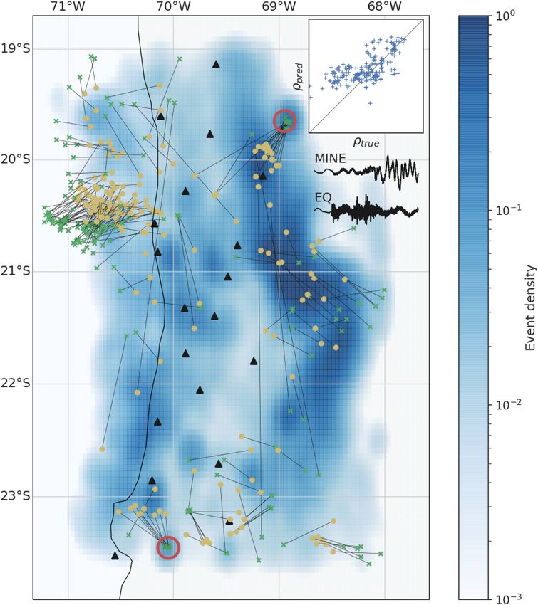
Figure 5. True and predicted magnitudes without upsampling or transfer learning (left-hand column), with upsampling but without transfer learning (middle
column) and with upsampling and transfer learning (right-hand column). All plots show predictions after 8 s. In the transfer column for Chile and Japan we
show results after fine-tuning on the target data set; for Italy we show results from the model without fine-tuning as this model performed better. For the largest
events in Italy (M > 4.5) we additionally show the results after fine-tuning with pale blue dots. We suspect the degraded performance in the fine tuned model
results from the fact, that the largest training event (MW = 6.1) is considerably smaller than the largest test event (MW = 6.5). Vertical lines indicate the
borders between small, medium and large events as defined in Fig. 4. The orange lines show the running 5th, 50th and 95th percentile in 0.2 m.u. buckets.
Percentile lines are only shown if sufficiently many data points are available. The very strong outlier for Japan (true ∼7.3, predicted ∼3.3) is an event far
offshore (>2000 km).
For magnitude estimation no consistent performance differences baseline with embeddings is even higher than the gains from adding
between the baseline approach with position embeddings and the the transformer to the embedding model. We speculate that the po-
approach with concatenated coordinates, as originally proposed by sitional embeddings might show better performance because they
van den Ende & Ampuero (2020), are visible. In contrast, for lo- explicity encode information on how to interpolate between loca-
cation estimation, the approach with embeddings consistently out- tions at different scales, enabling an improved exploitation of the
performs the approach with concatenated coordinates. The absolute information from stations with few or no training examples. This
performance gains between the baseline with concatenation and the is more important for location estimation, where an explicit notionEarthquake assessment with TEAM-LM 1095
learning (Pan & Yang 2009), in our use case waveforms from other
source regions. This way the model is supposed to be taught the
properties of earthquakes that are consistent across regions, for
example attenuation due to geometric spreading or the magnitude
dependence of source spectra. Note that a similar knowledge transfer
implicitly is part of the classical baseline, as it was calibrated using
records from multiple regions.
Here, we conduct a transfer learning experiment inspired by the
Downloaded from https://academic.oup.com/gji/article/226/2/1086/6223459 by Bibliothek des Wissenschaftsparks Albert Einstein user on 14 June 2021
transfer learning used for TEAM. We first train a model jointly on all
data sets and then fine-tune it to each of the target data sets. This way,
the model has more training examples, which is of special relevance
for the rare large events, but still is adapted specifically to the target
data set. As the Japan and Italy data sets contain acceleration traces,
while the Chile data set contains velocity traces, we first integrate
the Japan and Italy waveforms to obtain velocity traces. This does
not have a significant impact on the model performance, as visible
in the full results tables (Tables S5–S8).
Transfer learning reduces the saturation for large magnitudes
(Fig. 5, right-hand column). For Italy the saturation is even com-
pletely eliminated. For Chile, while the largest magnitudes are still
underestimated, we see a clearly lower level of underestimation
than without transfer learning. Results for Japan for the largest
events show nearly no difference, which is expected as the Japan
data set contains the majority of large events and therefore does
not gain significant additional large training examples using trans-
fer learning. The positive impact of transfer learning is also re-
flected in the lower RMSE for large and intermediate events for
Italy and Chile (Fig. 4). These results do not only offer a way
of mitigating saturation for large events, but also represent fur-
ther evidence for data sparsity as the reason for the underestima-
tion.
We tried the same transfer learning scheme for mitigating mis-
locations (Fig. 6). For this experiment we shifted the coordinates
of stations and events such that the data sets spatially overlap. We
note that this shifting is not expected to have any influence on
the single data set performance, as the relative locations of events
and stations within a data set stay unchanged and nowhere the
model uses absolute locations. The transfer learning approach is
reasonable, as mislocations might result from data sparsity, simi-
larly to the underestimation of large magnitudes. However, none
of the models shows significantly better performance than the
preferred models, and in some instances performance even de-
grades. We conducted additional experiments where shifts were
applied separately for each event, but observed even worse perfor-
mance.
Figure 6. Violin plots and error quantiles of the distributions of the epicen- We hypothesize that this behaviour indicates that the TEAM-
tral errors for TEAM-LM, the pooling baseline with position embeddings
LM localization does not primarily rely on traveltime analysis, but
(POOL-E), the pooling baseline with concatenated position (POOL-C),
TEAM-LM with transfer learning (TEAM-TRA) and a classical baseline.
rather uses some form of fingerprinting of earthquakes. These fin-
Vertical lines mark the 50th, 90th, 95th and 99th error percentiles, with gerprints could be specific scattering patterns for certain source
smaller markers indicating higher quantiles. The time indicates the time regions and receivers. Note that similar fingerprints are exploited
since the first P arrival at any station. We compute errors based on the mean in the traditional template matching approaches (e.g. Shelly et al.
location predictions. A similar plot for hypocentral errors is available in the 2007). While the traveltime analysis should be mostly invariant
supplementary material (Fig. S4). to shifts and therefore be transferable between data sets, the fin-
gerprinting is not invariant to shifts. This would also explain why
of relative position is required. In contrast, magnitude estimation the transfer learning, where all training samples were already in
can use further information, like frequency content, which is less the pretraining data set and therefore their fingerprints could be
position dependent. extracted, outperforms the shifting of single events, where finger-
prints do not relate to earthquake locations. Similar fingerprinting
is presumably also used by other deep learning methods for location
3.3 Transfer learning
estimation, for example by Kriegerowski et al. (2019) or Perol et al.
A common strategy for mitigating data sparsity is the injection (2018), however further experiments would be required to prove this
of additional information from related data sets through transfer hypothesis.1096 J. Münchmeyer et al.
4 DISCUSSION In contrast to traditional algorithms, events are not only predicted
to be closer to the network, but they are also predicted as lying
4.1 Multitask learning in regions with a higher event density in the training set (Fig. 7,
inset). This suggests that not enough similar events were included
Another common method to improve the quality of machine learn-
in the training data set. Similarly, Kriegerowski et al. (2019) ob-
ing systems in face of data sparsity is multitask learning (Ruder
served a clustering tendency when predicting the location of swarm
2017), that is having a network with multiple outputs for differ-
earthquakes with deep learning.
ent objectives and training it simultaneously on all objectives. This
We investigated two subgroups of mislocated events: the Iquique
Downloaded from https://academic.oup.com/gji/article/226/2/1086/6223459 by Bibliothek des Wissenschaftsparks Albert Einstein user on 14 June 2021
approach has previously been used for seismic source characteriza-
sequence, consisting of the Iquique main shock, foreshocks and
tion (Lomax et al. 2019), but without an empirical analysis on the
aftershocks, and mine blasts. The Iquique sequence is visible in
specific effects of multitask learning.
the north-western part of the study area. All events are predicted
We perform an experiment, in which we train TEAM-LM to
approximately 0.5◦ too far east. The area is both outside the seis-
predict magnitude and location concurrently. The feature extraction
mic network and has no events in the training set. This systematic
and the transformer parts are shared and only the final MLPs and
mislocation may pose a serious threat in applications, such as early
the mixture density networks are specific to the task. This method is
warning, when confronted with a major change in the seismicity
known as hard parameter sharing. The intuition is that the individual
pattern, as is common in the wake of major earthquakes or during
tasks share some similarity, for example in our case the correct
sudden swarm activity, which are also periods of heightened seismic
estimation of the magnitude likely requires an assessment of the
hazard.
attenuation and geometric spreading of the waves and therefore
For mine blasts, we see one mine in the northeast and one in the
some understanding of the source location. This similarity is then
southwest (marked by red circles in Fig. 7). While all events are
expected to drive the model towards learning a solution for the
located close by, the location are both systematically mispredicted
problem that is more general, rather than specific to the training data.
in the direction of the network and exhibit scatter. Mine-blasts show
The reduced number of free parameters implied by hard parameter
a generally lower location quality in the test set. While they make
sharing is also expected to improve the generality of the derived
up only ∼1.8 per cent of the test set, they make up 8 per cent of
model, if the remaining degrees of freedom are still sufficient to
the top 500 mislocated events. This is surprising as they occur not
extract the relevant information from the training data for each
only in the test set, but also in similar quantities in the training set.
subtask.
We therefore suspect that the difficulties are caused by the strongly
Unfortunately, we actually experience a moderate degradation of
different waveforms of mine blasts compared to earthquakes. One
performance for either location or magnitude in any data set (Tables
waveform of each a mine blast and an earthquake, recorded at similar
S5–S11) when following a multitask learning strategy. The RMSE
distances are shown as inset in Fig. 7. While for the earthquake both
of the mean epicentre estimate increases by at least one third for
a P and S wave are visible, the S wave can not be identified for the
all times and data sets, and the RMSE for magnitude stays nearly
mine blast. In addition, the mine blast exhibits a strong surface wave,
unchanged for the Chile and Japan data sets, but increases by ∼20
which is not visible for the earthquake. The algorithm therefore can
per cent for the Italy data set. Our results therefore exhibit a case of
not use the same features as for earthquakes to constrain the distance
negative transfer.
to a mine blast event.
While it is generally not known, under which circumstances mul-
titask learning shows positive or negative influence (Ruder 2017),
a negative transfer usually seems to be caused by insufficiently re-
lated tasks. In our case we suspect that while the tasks are related
in a sense of the underlying physics, the training data set is large 4.3 The impact of data set size and composition
enough that similarities relevant for both tasks can be learned al-
Our analysis so far showed the importance of the amount of training
ready from a single objective. At the same time, the particularities
data. To quantify the impact of data availability on magnitude and
of the two objectives can be learned less well. Furthermore, we ear-
location estimation, we trained models only using fractions of the
lier discussed that both magnitude and location might not actually
training and validation data (Fig. 8). We use the Chile data set for
use traveltime or attenuation based approaches, but rather frequency
this analysis, as it contains by far the most events. We subsample
characteristics for magnitude and a fingerprinting scheme for loca-
the events by only using each kth event in chronological order, with
tion. These approaches would be less transferable between the two
k = 2, 4, 8, 16, 32, 64. This strategy approximately maintains the
tasks. We conclude that hard parameter sharing does not improve
magnitude and location distribution of the full set. We point out, that
magnitude and location estimation. Future work is required to see
TEAM-LM only uses information of the event under consideration
if other multitask learning schemes can be applied beneficially.
and does not take the events before or afterwards into account.
Therefore, the ‘gaps’ between events introduced by the subsampling
do not negatively influence TEAM-LM.
4.2 Location outlier analysis
For all times after the first P arrival, we see a clear increase in the
As all location error distributions are heavy tailed, we visually in- magnitude-RMSE for a reduction in the number of training samples.
spect the largest deviations between predicted and catalogue loca- While the impact of reducing the data set by half is relatively small,
tions to understand the behavior of the localization mechanism of using only a quarter of the data already leads to a twofold increase
TEAM-LM. We base this analysis on the Chile data set (Fig. 7), in RMSE at late times. Even more relevant in an early warning
as it has generally the best location estimation performance, but context, a fourfold smaller data sets results in an approximately
observations are similar for the other data sets (Figs S5 and S6). fourfold increase in the time needed to reach the same precision as
Nearly all mislocated events are outside the seismic network and with the full data. This relationship seems to hold approximately
location predictions are generally biased towards the network. This across all subsampled data sets: reducing the data set k fold increases
matches the expected errors for traditional localization algorithms. the time to reach a certain precision by a factor of k.Earthquake assessment with TEAM-LM 1097 Figure 7. The 200 events with the highest location errors in the Chile data set overlayed on top of the spatial event density in the training data set. The location Downloaded from https://academic.oup.com/gji/article/226/2/1086/6223459 by Bibliothek des Wissenschaftsparks Albert Einstein user on 14 June 2021 estimations use 16 s of data. Each event is denoted by a yellow dot for the estimated location, a green cross for the true location and a line connecting both. Stations are shown by black triangles. The event density is calculated using a Gaussian kernel density estimation and does not take into account the event depth. The inset shows the event density at the true event location in comparison to the event density at the predicted event location for the 200 events. Red circles mark locations of mine blast events. The inset waveforms show one example of a waveform from a mineblast (top) and an example waveform of an earthquake (bottom, 26 km depth) of similar magnitude (MA = 2.5) at similar distance (60 km) on the transverse component. Similar plots for Italy and Japan can be found in the supplementary material (Figs S5 and S6). We make three further observations from comparing the pre- underestimated. In addition, for 1/32 and 1/64 of the full data set, an dictions to the true values (Fig. S7). First, for nearly all models the ‘inverse saturation’ effect is noticeable for the smallest magnitudes. RMSE changes only marginally between 16 and 25 s, but the RMSE Thirdly, while for the full data set and the largest subsets all large of this plateau increases significantly with a decreasing number of events are estimated at approximately the saturation threshold, if training events. Secondly, the lower the amount of training data, the at most one quarter of the training data is used, the largest events lower is the saturation threshold above which all events are strongly even fall significantly below the saturation threshold. For the mod-
1098        J. Münchmeyer et al.

                                                                                                                                                                     Downloaded from https://academic.oup.com/gji/article/226/2/1086/6223459 by Bibliothek des Wissenschaftsparks Albert Einstein user on 14 June 2021
Figure 8. RMSE for magnitude and epicentral location at different times for models trained on differently sized subsets of the training set in Chile. The line
colour encodes the fraction of the training and validation set used in training. All models were evaluated on the full Chilean test set. We note that the variance
of the curves with fewer data is higher, due to the increased stochasticity from model training and initialization.

Figure 9. Magnitude predictions and uncertainties in the Chile data set as a function of time since the first P arrival. Solid lines indicate median predictions,
while dashed lines (left-hand panel only) show 20th and 80th quantiles of the prediction. The left-hand panel shows the predictions, while the right-hand
panel shows the differences between the predicted and true magnitude. The right-hand panel is focused on a shorter time frame to show the early prediction
development in more detail. In both plots, each colour represents a different magnitude bucket. For each magnitude bucket, we sampled 1000 events around
this magnitude and combined their predictions. If less than 1000 events were available within ±0.5 m.u. of the bucket centre, we use all events within this
range. We only use events from the test set. To ensure that the actual uncertainty distribution is visualized, rather than the distribution of magnitudes around
the bucket centre, each prediction is shifted by the magnitude difference between bucket centre and catalogue magnitude.

els trained on the smallest subsets (1/8 to 1/64), the higher the true              are available. This demonstrates that location estimation with
magnitude the lower the predicted magnitude becomes. We assume                      high accuracy requires catalogues with a high event den-
that the larger the event is, the further away from the training distri-            sity.
bution it is and therefore it is estimated approximately at the most                   The strong degradation further suggests insights into the inner
dense region of the training label distribution. These observations                 working of TEAM-LM. Classically, localization should be a task
support the hypothesis that underestimations of large magnitudes                    where interpolation leads to good results, i.e., the traveltimes for
for the full data set are caused primarily by insufficient training                 an event in the middle of two others should be approximately the
data.                                                                               average between the traveltimes for the other events. Following this
   While the RMSE for epicentre estimation shows a similar                          argument, if the network would be able to use interpolation, it should
behavior as the RMSE for magnitude, there are subtle dif-                           not suffer such significant degradation when faced with fewer data.
ferences. If the amount of training data is halved, the per-                        This provides further evidence that the network does not actually
formance only degrades mildly and only at later times. How-                         learn some form of triangulation, but only an elaborate fingerprint-
ever, the performance degradation is much more severe than                          ing scheme, backing the finding from the qualitative analysis of
for magnitude if only a quarter or less of the training data                        location errors.
Earthquake assessment with TEAM-LM 1099
4.4 Training TEAM-LM on large events only
Often, large events are of the greatest concerns, and as discussed,
generally showed poorer performance because they are not well
represented in the training data. It therefore appears plausible that
a model optimized for large events might perform better than a
model trained on both large and small events. In order to test this
hypothesis, we used an extreme version of the upscaling strategy
Downloaded from https://academic.oup.com/gji/article/226/2/1086/6223459 by Bibliothek des Wissenschaftsparks Albert Einstein user on 14 June 2021
by training a set of models only on large events, which might avoid
tuning the model to seemingly irrelevant small events. In fact, these
models perform significantly worse than the models trained on the
full data set, even for the large events (Tables S5–S11). Therefore
even if the events of interest are only the large ones, training on
more complete catalogues is still beneficial, presumably by giv-
ing the network more comprehensive information on the regional
propagation characteristics and possibly site effects.
4.5 Interpretation of predicted uncertainties
So far we only analysed the mean predictions of TEAM-LM. As
for many application scenarios, for example early warning, quanti-
fied uncertainties are required, TEAM-LM outputs not only these
mean predictions, but a probability density. Fig. 9 shows the devel-
opment of magnitude uncertainties for events from different mag-
nitude classes in the Chile data set. The left-hand panel shows the
absolute predictions, while the right-hand panel shows the differ-
ence between prediction and true magnitude and focuses on the first
2 s. As we average over multiple events, each set of lines can be
seen as a prototype event of a certain magnitude.
For all magnitude classes the estimation shows a sharp jump at
t = 0, followed by a slow convergence to the final magnitude esti-
mate. We suspect that the magnitude estimation always converges
from below, as due to the Gutenberg–Richter distribution, lower
magnitudes are more likely a priori. The uncertainties are largest
directly after t = 0 and subsequently decrease, with the highest un-
certainties for the largest events. As we do not use transfer learning
in this approach, there is a consistent underestimation of the largest
magnitude events, visible from the incorrect median predictions for
magnitudes 5 and 6. We note that the predictions for magnitude
4 converge slightly faster than the ones for magnitude 3, while in
all other cases the magnitude convergence is faster the smaller the
events are. We suspect that this is caused by the accuracy of the
magnitude estimation being driven by both the number of available
events and by the signal to noise ratio. While magnitude 4 events
have significantly less training data than magnitude 3 events, they
have a better signal to noise ratio, which could explain their more
accurate early predictions.
While the Gaussian mixture model is designed to output uncer-
Figure 10. P-P plots of the CDFs of the empirical quantile of the magnitude tainties, it cannot be assumed that the predicted uncertainties are
predictions compared to the expected uniform distribution. The P-P plot indeed well calibrated, that is, that they actually match the real er-
shows (CDFu i (z), CDFuniform (z)) for z ∈ [0, 1]. The expected uniform dis- ror distribution. Having well calibrated uncertainties is crucial for
tribution is shown as the diagonal line, the misfit is indicated as shaded area. downstream tasks that rely on the uncertainties. Neural networks
The value in the upper corner provides d∞ , the maximum distance between
trained with a log-likelihood loss generally tend to be overconfi-
the diagonal and the observed CDF. d∞ can be interpreted as the test statis-
tic for a Kolmogorov–Smirnov test. Curves consistently above the diagonal
dent (Snoek et al. 2019; Guo et al. 2017), that is underestimate the
indicate a bias to underestimation, and below the diagonal to overestima- uncertainties. This overconfidence is probably caused by the strong
tion. Sigmoidal curves indicate overconfidence, mirrored sigmoids indicate overparametrization of neural network models. To assess the quality
underconfidence. See supplementary section SM 2 for a further discussion of our uncertainty estimations for magnitude, we use the observation
of the plotting methodology and its connection to the Kolmogorov–Smirnov that for a specific event i, the predicted Gaussian mixture implies a
ed : R → [0, 1]. Given the ob-
test. i
cumulative distribution function Fpr
served magnitude ytr ue , we can calculate u i = Fpr
i i i i
ed (ytr ue ). If ytr ue isYou can also read