Natural Language Processing with Deep Learning CS224N/Ling284 - John Hewitt Lecture 9: Self-Attention and Transformers - Natural Language ...

Natural Language Processing
 with Deep Learning
 CS224N/Ling284

 John Hewitt
 Lecture 9: Self-Attention and Transformers

Lecture Plan
1. From recurrence (RNN) to attention-based NLP models
2. Introducing the Transformer model
3. Great results with Transformers
4. Drawbacks and variants of Transformers

Reminders:
 Assignment 4 due on Thursday!
 Mid-quarter feedback survey due Tuesday, Feb 16 at 11:59PM PST!
 Final project proposal due Tuesday, Feb 16 at 4:30PM PST!
 Please try to hand in the project proposal on time; we want to get you feedback
 quickly!

2

As of last week: recurrent models for (most) NLP!

• Circa 2016, the de facto strategy in NLP is to
 encode sentences with a bidirectional LSTM:
 (for example, the source sentence in a translation)

• Define your output (parse, sentence,
 summary) as a sequence, and use an LSTM to
 generate it.

• Use attention to allow flexible access to
 memory

3

Today: Same goals, different building blocks

• Last week, we learned about sequence-to-sequence problems and
 encoder-decoder models.
• Today, we’re not trying to motivate entirely new ways of looking at
 problems (like Machine Translation)
• Instead, we’re trying to find the best building blocks to plug into our
 models and enable broad progress.

 Lots of trial
 and error

 2014-2017ish 2021
 Recurrence ??????
4

Issues with recurrent models: Linear interaction distance

• RNNs are unrolled “left-to-right”.
• This encodes linear locality: a useful heuristic!
 • Nearby words often affect each other’s meanings
 tasty pizza
• Problem: RNNs take O(sequence length) steps for
 distant word pairs to interact.

 O(sequence length)

 The chef who … was
5

Issues with recurrent models: Linear interaction distance

• O(sequence length) steps for distant word pairs to interact means:
 • Hard to learn long-distance dependencies (because gradient problems!)
 • Linear order of words is “baked in”; we already know linear order isn’t the
 right way to think about sentences…

 The chef who … was
 Info of chef has gone through
 O(sequence length) many layers!
6

Issues with recurrent models: Lack of parallelizability

• Forward and backward passes have O(sequence length)
 unparallelizable operations
 • GPUs can perform a bunch of independent computations at once!
 • But future RNN hidden states can’t be computed in full before past RNN
 hidden states have been computed
 • Inhibits training on very large datasets!

 1 2 3 T

 0 1 2 T-1

 h1 h2 hT

 Numbers indicate min # of steps before a state can be computed
7

If not recurrence, then what? How about word windows?

• Word window models aggregate local contexts
 • (Also known as 1D convolution; we’ll go over this in depth later!)
 • Number of unparallelizable operations does not increase sequence length!

 2 2 2 2 2 2 2 2
 window
 1 1 1 1 1 1 1 1
 window
 embedding 0 0 0 0 0 0 0 0
 h1 h2 hT

 Numbers indicate min # of steps before a state can be computed
8

If not recurrence, then what? How about word windows?

• Word window models aggregate local contexts
• What about long-distance dependencies?
 • Stacking word window layers allows interaction between farther words
• Maximum Interaction distance = sequence length / window size
 • (But if your sequences are too long, you’ll just ignore long-distance context)

 window (size=5) Red states
 indicate those
 window (size=5) “visible” to hk
 embedding
 h1 hk hT

9
 Too far from hk to be considered

If not recurrence, then what? How about attention?

• Attention treats each word’s representation as a query to access and
 incorporate information from a set of values.
 • We saw attention from the decoder to the encoder; today we’ll think about
 attention within a single sentence.
• Number of unparallelizable operations does not increase sequence length.
• Maximum interaction distance: O(1), since all words interact at every layer!

 2 2 2 2 2 2 2 2
 All words attend
 attention to all words in
 1 1 1 1 1 1 1 1 previous layer;
 attention
 most arrows here
 0 0 0 0 0 0 0 0 are omitted
 embedding
 h1 h2 hT
10

Self-Attention

 • Recall: Attention operates on queries, keys, and values.
 The number of queries
 
 • We have some queries 1 , 2 , … , . Each query is ∈ ℝ can differ from the
 • We have some keys 1 , 2 , … , . Each key is ∈ ℝ number of keys and
 values in practice.
 • We have some values 1 , 2 , … , . Each value is ∈ ℝ 
 • In self-attention, the queries, keys, and values are drawn from the same source.
 • For example, if the output of the previous layer is 1 , … , , (one vec per word)
 we could let = = = (that is, use the same vectors for all of them!)
 • The (dot product) self-attention operation is as follows:
 exp( )
 = ⊤ = output = ෍ 
 σ ′ exp( ′ ) 
 Compute key- Compute attention Compute outputs as
 query affinities weights from affinities weighted sum of values
11 (softmax)

Self-attention as an NLP building block

 • In the diagram at the right, we
 have stacked self-attention
 blocks, like we might stack LSTM self-attention
 layers. 1 1 1 2 2 2 3 3 3 

 • Can self-attention be a drop-in
 …
 replacement for recurrence? self-attention
 1 1 1 2 2 2 3 3 3 
 • No. It has a few issues, which
 we’ll go through. …
 1 2 3 
 • First, self-attention is an The chef who food
 operation on sets. It has no
 inherent notion of order. Self-attention doesn’t know the order of its inputs.
12

Barriers and solutions for Self-Attention as a building block

 Barriers Solutions
 • Doesn’t have an inherent
 notion of order!

13

Fixing the first self-attention problem: sequence order

 • Since self-attention doesn’t build in order information, we need to encode the order of the
 sentence in our keys, queries, and values.
 • Consider representing each sequence index as a vector
 ∈ ℝ , for ∈ {1,2, … , } are position vectors

 • Don’t worry about what the are made of yet!
 • Easy to incorporate this info into our self-attention block: just add the to our inputs!
 • Let ෤ ෨ , ෤ be our old values, keys, and queries.

 = ෤ + In deep self-attention
 = ෤ + networks, we do this at the
 = ෨ + first layer! You could
 concatenate them as well,
 but people mostly just add…
14

Position representation vectors through sinusoids

 • Sinusoidal position representations: concatenate sinusoidal functions of varying periods:

 sin( /100002∗1/ )
 cos( /100002∗1/ )

 Dimension
 =
 
 2∗ 2 / 
 sin( /10000 )
 
 cos( /100002∗2 / ) Index in the sequence
 • Pros:
 • Periodicity indicates that maybe “absolute position” isn’t as important
 • Maybe can extrapolate to longer sequences as periods restart!
 • Cons:
 • Not learnable; also the extrapolation doesn’t really work!

15 Image: https://timodenk.com/blog/linear-relationships-in-the-transformers-positional-encoding/

Position representation vectors learned from scratch

 • Learned absolute position representations: Let all be learnable parameters!
 Learn a matrix ∈ ℝ × , and let each be a column of that matrix!

 • Pros:
 • Flexibility: each position gets to be learned to fit the data
 • Cons:
 • Definitely can’t extrapolate to indices outside 1, … , .
 • Most systems use this!

 • Sometimes people try more flexible representations of position:
 • Relative linear position attention [Shaw et al., 2018]
 • Dependency syntax-based position [Wang et al., 2019]

16

Barriers and solutions for Self-Attention as a building block

 Barriers Solutions
 • Doesn’t have an inherent • Add position representations to
 notion of order! the inputs

 • No nonlinearities for deep
 learning! It’s all just weighted
 averages

17

Adding nonlinearities in self-attention

• Note that there are no elementwise
 nonlinearities in self-attention;
 stacking more self-attention layers FF FF FF FF
 just re-averages value vectors
 self-attention

• Easy fix: add a feed-forward network
 …
 to post-process each output vector. FF FF FF FF

 = output self-attention
 = 2 ∗ ReLU 1 × output + 1 + 2 …
 1 2 3 
 The chef who food

 Intuition: the FF network processes the result of attention
18

Barriers and solutions for Self-Attention as a building block

 Barriers Solutions
 • Doesn’t have an inherent • Add position representations to
 notion of order! the inputs

 • No nonlinearities for deep • Easy fix: apply the same
 learning magic! It’s all just feedforward network to each self-
 weighted averages attention output.

 • Need to ensure we don’t
 “look at the future” when
 predicting a sequence
 • Like in machine translation
 • Or language modeling
19

Masking the future in self-attention
 We can look at these
 (not greyed out) words
• To use self-attention in
 decoders, we need to ensure
 we can’t peek at the future.

 [START] −∞ −∞ −∞ −∞
• At every timestep, we could
 change the set of keys and
 queries to include only past The −∞ −∞ −∞
 words. (Inefficient!) For encoding
 these words
 chef −∞ −∞
• To enable parallelization, we
 mask out attention to future
 words by setting attention who −∞
 scores to −∞. ⊤ , < 
 = ൝
 −∞, ≥ 
20 [The matrix of values]

Masking the future in self-attention
 We can look at these
 (not greyed out) words
• To use self-attention in
 decoders, we need to ensure
 we can’t peek at the future.

 [START] −∞ −∞ −∞ −∞
• At every timestep, we could
 change the set of keys and
 queries to include only past The −∞ −∞ −∞
 words. (Inefficient!) For encoding
 these words
 chef −∞ −∞
• To enable parallelization, we
 mask out attention to future
 words by setting attention who −∞
 scores to −∞. ⊤ , < 
 = ൝
 −∞, ≥ 
21

Barriers and solutions for Self-Attention as a building block

 Barriers Solutions
 • Doesn’t have an inherent • Add position representations to
 notion of order! the inputs

 • No nonlinearities for deep • Easy fix: apply the same
 learning magic! It’s all just feedforward network to each self-
 weighted averages attention output.

 • Need to ensure we don’t • Mask out the future by artificially
 “look at the future” when setting attention weights to 0!
 predicting a sequence
 • Like in machine translation
 • Or language modeling
22

Necessities for a self-attention building block:

 • Self-attention:
 • the basis of the method.
 • Position representations:
 • Specify the sequence order, since self-attention is an unordered function of its
 inputs.
 • Nonlinearities:
 • At the output of the self-attention block
 • Frequently implemented as a simple feed-forward network.
 • Masking:
 • In order to parallelize operations while not looking at the future.
 • Keeps information about the future from “leaking” to the past.

 • That’s it! But this is not the Transformer model we’ve been hearing about.
23

Outline
1. From recurrence (RNN) to attention-based NLP models
2. Introducing the Transformer model
3. Great results with Transformers
4. Drawbacks and variants of Transformers

24

The Transformer Encoder-Decoder [Vaswani et al., 2017]
First, let’s look at the Transformer Encoder and Decoder Blocks at a high level
 [predictions!]

 Transformer Transformer
 Encoder Decoder
 [decoder attends
 to encoder states]

 Transformer Transformer
 Encoder Decoder

 Word + Position Word Position
 +
 Embeddings Representations Embeddings Representations

 [input sequence] [output sequence]
25

The Transformer Encoder-Decoder [Vaswani et al., 2017]
Next, let’s look at the Transformer Encoder and Decoder Blocks

What’s left in a Transformer Encoder Block that we haven’t covered?
1. Key-query-value attention: How do we get the , , vectors from a single word embedding?
2. Multi-headed attention: Attend to multiple places in a single layer!
3. Tricks to help with training!
 1. Residual connections
 2. Layer normalization
 3. Scaling the dot product
 4. These tricks don’t improve what the model is able to do; they help improve the training process.
 Both of these types of modeling improvements are very important!

26

The Transformer Encoder: Key-Query-Value Attention

 • We saw that self-attention is when keys, queries, and values come from the same
 source. The Transformer does this in a particular way:
 • Let 1 , … , be input vectors to the Transformer encoder; ∈ ℝ 

 • Then keys, queries, values are:
 • = , where ∈ ℝ × is the key matrix.
 • = , where Q ∈ ℝ × is the query matrix.
 • = , where V ∈ ℝ × is the value matrix.

 • These matrices allow different aspects of the vectors to be used/emphasized in
 each of the three roles.

27

The Transformer Encoder: Key-Query-Value Attention

 • Let’s look at how key-query-value attention is computed, in matrices.
 • Let = 1 ; … ; ∈ ℝ × be the concatenation of input vectors.
 • First, note that ∈ ℝ × , ∈ ℝ × , ∈ ℝ × .
 • The output is defined as output = softmax ⊤ × .

 First, take the query-key dot All pairs of
 products in one matrix = ⊤ ⊤ attention scores!
 multiplication: ⊤ ⊤ ⊤ ∈ ℝ × 

 Next, softmax, and
 compute the weighted
 average with another
 softmax ⊤ ⊤ =
 output ∈ ℝ × 
 matrix multiplication.
28

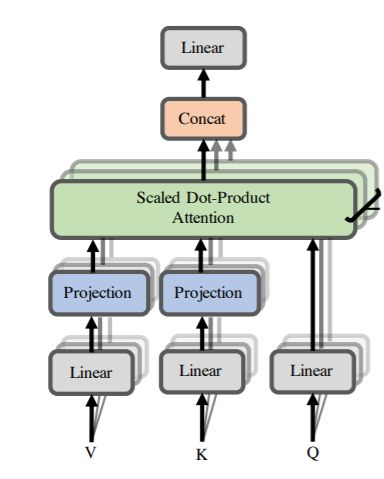
The Transformer Encoder: Multi-headed attention

 • What if we want to look in multiple places in the sentence at once?
 • For word , self-attention “looks” where ⊤ ⊤ is high, but maybe we want
 to focus on different for different reasons?
 • We’ll define multiple attention “heads” through multiple Q,K,V matrices
 
 ×ℎ
 • Let, ℓ , ℓ , ℓ ∈ ℝ , where ℎ is the number of attention heads, and ℓ ranges
 from 1 to ℎ.
 • Each attention head performs attention independently:
 • output ℓ = softmax ℓ ℓ⊤ ⊤ ∗ ℓ , where output ℓ ∈ ℝ /ℎ
 • Then the outputs of all the heads are combined!
 • output = [output1 ; … ; output ℎ ], where ∈ ℝ × 

 • Each head gets to “look” at different things, and construct value vectors
29
 differently.

The Transformer Encoder: Multi-headed attention

 • What if we want to look in multiple places in the sentence at once?
 • For word , self-attention “looks” where ⊤ ⊤ is high, but maybe we want
 to focus on different for different reasons?
 • We’ll define multiple attention “heads” through multiple Q,K,V matrices
 
 ×ℎ
 • Let, ℓ , ℓ , ℓ ∈ ℝ , where ℎ is the number of attention heads, and ℓ ranges
 from 1 to ℎ.

 Single-head attention Multi-head attention
 (just the query matrix) (just two heads here) Same amount of
 computation as
 single-head self-
 attention!
 1 2
 = 1 2 =
30

The Transformer Encoder: Residual connections [He et al., 2016]

 • Residual connections are a trick to help models train better.
 • Instead of ( ) = Layer( −1
 ) (where represents the layer)

 ( −1) Layer ( )

 • We let ( ) = ( −1) + Layer( −1
 ) (so we only have to learn “the residual”
 from the previous layer)
 ( −1) Layer + ( )

 • Residual connections are thought to make
 the loss landscape considerably smoother
 (thus easier training!) [no residuals] [residuals]
 [Loss landscape visualization,
31 Li et al., 2018, on a ResNet]

The Transformer Encoder: Layer normalization [Ba et al., 2016]

 • Layer normalization is a trick to help models train faster.
 • Idea: cut down on uninformative variation in hidden vector values by normalizing
 to unit mean and standard deviation within each layer.
 • LayerNorm’s success may be due to its normalizing gradients [Xu et al., 2019]
 • Let ∈ ℝ be an individual (word) vector in the model.
 • Let = σ =1 ; this is the mean; ∈ ℝ.
 1 2
 • Let = σ =1 − ; this is the standard deviation; ∈ ℝ.
 
 • Let ∈ ℝ and 
 ∈ ℝ be learned “gain” and “bias” parameters. (Can omit!)
 • Then layer normalization computes:
 − 
 output = ∗ + 
 + 
 Normalize by scalar Modulate by learned
32
 mean and variance elementwise gain and bias

The Transformer Encoder: Layer normalization [Ba et al., 2016]

 • Layer normalization is a trick to help models train faster.
 • Idea: cut down on uninformative variation in hidden vector values by normalizing
 to unit mean and standard deviation within each layer.
 • LayerNorm’s success may be due to its normalizing gradients [Xu et al., 2019]
 • Let ∈ ℝ be an individual (word) vector in the model.
 • Let = σ =1 ; this is the mean; ∈ ℝ.
 1 2
 • Let = σ =1 − ; this is the standard deviation; ∈ ℝ.
 
 • Let ∈ ℝ and 
 ∈ ℝ be learned “gain” and “bias” parameters. (Can omit!)
 • Then layer normalization computes:
 − 
 output = ∗ + 
 + 
 Normalize by scalar Modulate by learned
33
 mean and variance elementwise gain and bias

The Transformer Encoder: Scaled Dot Product [Vaswani et al., 2017]

 • “Scaled Dot Product” attention is a final variation to aid in Transformer training.
 • When dimensionality becomes large, dot products between vectors tend to
 become large.
 • Because of this, inputs to the softmax function can be large, making the
 gradients small.
 • Instead of the self-attention function we’ve seen:
 output ℓ = softmax ℓ ℓ⊤ ⊤ ∗ ℓ
 • We divide the attention scores by /ℎ, to stop the scores from becoming large
 just as a function of /ℎ (The dimensionality divided by the number of heads.)
 ℓ ℓ⊤ ⊤
 output ℓ = softmax ∗ ℓ
 /ℎ

34

The Transformer Encoder-Decoder [Vaswani et al., 2017]
Looking back at the whole model, zooming in on an Encoder block:
 [predictions!]

 Transformer Transformer
 Encoder Decoder
 [decoder attends
 to encoder states]

 Transformer Transformer
 Encoder Decoder

 Word + Position Word Position
 +
 Embeddings Representations Embeddings Representations

 [input sequence] [output sequence]
35

The Transformer Encoder-Decoder [Vaswani et al., 2017]
Looking back at the whole model, zooming in on an Encoder block:
 [predictions!]
 Transformer
 Encoder Transformer
 Decoder
 Residual + LayerNorm [decoder attends
 Feed-Forward to encoder states]

 Residual + LayerNorm
 Transformer
 Multi-Head Attention Decoder

 Word + Position Word Position
 +
 Embeddings Representations Embeddings Representations

 [input sequence] [output sequence]
36

The Transformer Encoder-Decoder [Vaswani et al., 2017]
 [predictions!]
Looking back at the whole model,
zooming in on a Decoder block: Transformer
 Decoder
 Transformer
 Encoder Residual + LayerNorm

 Feed-Forward

 Residual + LayerNorm
 Transformer
 Multi-Head Cross-Attention
 Encoder
 Residual + LayerNorm

 Word + Position Masked Multi-Head Self-Attention
 Embeddings Representations
 Word + Position
 [input sequence] Embeddings Representations

37
 [output sequence]

The Transformer Encoder-Decoder [Vaswani et al., 2017]
 [predictions!]
The only new part is attention from decoder to encoder.
Like we saw last week! Transformer
 Decoder
 Transformer
 Encoder Residual + LayerNorm

 Feed-Forward

 Residual + LayerNorm
 Transformer
 Multi-Head Cross-Attention
 Encoder
 Residual + LayerNorm

 Word + Position Masked Multi-Head Self-Attention
 Embeddings Representations
 Word + Position
 [input sequence] Embeddings Representations

38
 [output sequence]

The Transformer Decoder: Cross-attention (details)

 • We saw that self-attention is when keys, queries, and values come from the same
 source.
 • In the decoder, we have attention that looks more like what we saw last week.
 • Let ℎ1 , … , ℎ be output vectors from the Transformer encoder; ∈ ℝ 
 • Let 1 , … , be input vectors from the Transformer decoder, ∈ ℝ 
 • Then keys and values are drawn from the encoder (like a memory):
 • = ℎ , = ℎ .
 • And the queries are drawn from the decoder, = .

39

The Transformer Encoder: Cross-attention (details)

 • Let’s look at how cross-attention is computed, in matrices.
 • Let H = ℎ1 ; … ; ℎ ∈ ℝ × be the concatenation of encoder vectors.
 • Let Z = 1 ; … ; ∈ ℝ × be the concatenation of decoder vectors.
 • The output is defined as output = softmax ⊤ × .

 First, take the query-key dot All pairs of
 products in one matrix = ⊤ ⊤ attention scores!
 multiplication: ⊤ ⊤ ⊤ ∈ ℝ × 

 Next, softmax, and
 compute the weighted
 average with another
 softmax ⊤ ⊤ =
 output ∈ ℝ × 
 matrix multiplication.
40

Outline
1. From recurrence (RNN) to attention-based NLP models
2. Introducing the Transformer model
3. Great results with Transformers
4. Drawbacks and variants of Transformers

41

Great Results with Transformers
First, Machine Translation from the original Transformers paper!

 Not just better Machine Also more efficient to
 Translation BLEU scores train!
42 [Test sets: WMT 2014 English-German and English-French] [Vaswani et al., 2017]

Great Results with Transformers
 Next, document generation!

The old standard Transformers all the way down.

 43 [Liu et al., 2018]; WikiSum dataset

Great Results with Transformers
 Before too long, most Transformers results also included pretraining, a method we’ll
 go over on Thursday.
 Transformers’ parallelizability allows for efficient pretraining, and have made them
 the de-facto standard.

On this popular aggregate
benchmark, for example:

 All top models are
 Transformer (and
 pretraining)-based.

 More results Thursday when we discuss pretraining.
 44 [Liu et al., 2018]

Outline
1. From recurrence (RNN) to attention-based NLP models
2. Introducing the Transformer model
3. Great results with Transformers
4. Drawbacks and variants of Transformers

45

What would we like to fix about the Transformer?

 • Quadratic compute in self-attention (today):
 • Computing all pairs of interactions means our computation grows
 quadratically with the sequence length!
 • For recurrent models, it only grew linearly!
 • Position representations:
 • Are simple absolute indices the best we can do to represent position?
 • Relative linear position attention [Shaw et al., 2018]
 • Dependency syntax-based position [Wang et al., 2019]

46

Quadratic computation as a function of sequence length

 • One of the benefits of self-attention over recurrence was that it’s highly
 parallelizable.
 • However, its total number of operations grows as 2 , where is the
 sequence length, and is the dimensionality.

 Need to compute all
 = ⊤ ⊤ pairs of interactions!
 ⊤ ⊤ 2 
 ∈ ℝ × 

 • Think of as around , .
 • So, for a single (shortish) sentence, ≤ 30; 2 ≤ .
 • In practice, we set a bound like = 512.
 • But what if we’d like ≥ , ? For example, to work on long documents?

47

Recent work on improving on quadratic self-attention cost

 • Considerable recent work has gone into the question, Can we build models like
 Transformers without paying the 2 all-pairs self-attention cost?
 • For example, Linformer [Wang et al., 2020]

 Inference time (s)
 Key idea: map the
 sequence length
 dimension to a lower-
 dimensional space for
 values, keys

 Sequence length / batch size

48

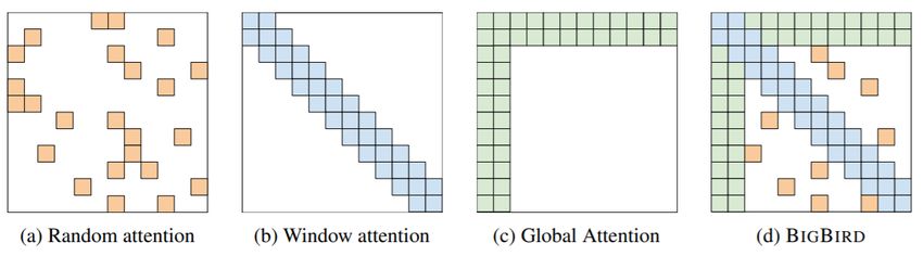
Recent work on improving on quadratic self-attention cost

 • Considerable recent work has gone into the question, Can we build models like
 Transformers without paying the 2 all-pairs self-attention cost?
 • For example, BigBird [Zaheer et al., 2021]

 Key idea: replace all-pairs interactions with a family of other interactions, like local
 windows, looking at everything, and random interactions.

49

Parting remarks

 • Pretraining on Thursday!
 • Good luck on assignment 4!
 • Remember to work on your project proposal!

50