Netflix Competition CptS 570 Machine Learning Project: Parisa Rashidi - Team: MLSurvivors
←
→
Page content transcription
If your browser does not render page correctly, please read the page content below
CptS 570 Machine
 Learning Project:
Netflix Competition

   Team: MLSurvivors
   Parisa Rashidi
Vikramaditya Jakkula

Wednesday, December 12, 2007
Introduction
In current report, we describe our efforts put forth the Netflix competition project as part
of the objectives for machine learning course, CptS570. Netflix, as a movie renting
company has developed a movie recommendation system called CinematchSM which its
job is to predict whether someone will enjoy a movie based on how much they liked or
disliked other movies by predicting a rating on a scale of 1-5 for the given movie. They
announced a contest carrying an award of $1 million for achieving 10% more accuracy
over current Cinematch prediction and progress award of $50k for best program
achieving 1% more accuracy over a declared RMSE.
Following is a brief description of the dataset:
There are 17770 movies.
There are 480189 users. CustomerIDs range from 1 to 2649429, with gaps.
Ratings are based on a scale of 1 to 5.
YearOfRelease range from 1890 to 2005.
Training set consists of 100 million records.
Qualifying dataset size is 2817131. It contains from 1-9999 movies ids.
Prediction needs to be submitted on this dataset.
Probe dataset size is 1408395. It contains from 1-9999 movies ids. This
dataset is meant to be used for checking the RMSE before proceeding for
qualifying dataset prediction.
Developing a solution for the Netflix project requires designing a recommender based
system. All of recommendation systems use the principal collaborative filtering in one
way or the other way. Collaborative filtering (CF) is the method of making automatic
predictions (filtering) about the interests of a user by collecting taste information from
many users (collaborating). The underlying assumption of CF approach is that: those who
agreed in the past tend to agree again in the future. A lot of research has been done in this
field giving birth to item-based filtering, user based filtering, content-based predictions
and many mixture models. For example in user based filtering, the user of the system
provides ratings of some artifacts or items. The system makes informed guesses about
other items the user may like based on ratings other users have provided. This is the
framework for social filtering methods. In item-based filtering, the system accepts
information describing the nature of an item and based on a sample of the user’s
preferences and learns to predict which items the user will like, usually called content
based filtering as it does not rely on social information, in the form of other users’
ratings. We aim to approach this problem using several different approaches such as
simple average, double average, nearest neighborhood coupled with movie information,
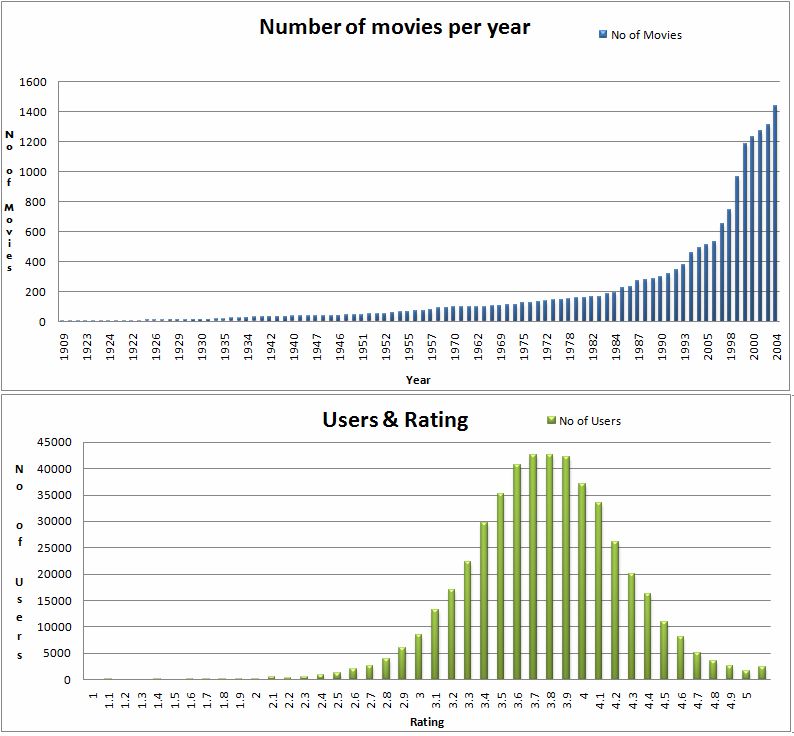
matrix factorization and slope one method.Netflix Data The Netflix data consists of a training set, of over 100 million ratings that over 480,000 users gave to nearly 18,000 movies. Each training rating is a quadruplet . The qualifying data set contains over 2.8 million triplets , with grades known only to the jury. A participating team's algorithm must predict grades on the entire qualifying set, but they are only informed of the score for half of the data, the quiz set. The other half is the test set, and performance on this is used by the jury to determine potential prize winners. Only the judges know which ratings are in the quiz set, and which are in the test set. Submitted predictions are scored against the true grades in terms of root mean squared error (RMSE), and the goal is to reduce this error as much as possible [5]. Another major hurdle in this dataset is missing data handling. Figure 1. Some interesting findings from the provided dataset. [Note: The charts plotted here are customized for the view to have a quick overview as how the dataset looks like. Also there are missing values] [6]
Methods Discussion
There are more than 23882 different teams registered on Netflix website, who are trying
to make improvements to their current algorithms with a variety of different methods and
techniques. Cinematch does straightforward statistical linear models with a lot of data
conditioning. But a real-world system is much more than an algorithm, and Cinematch
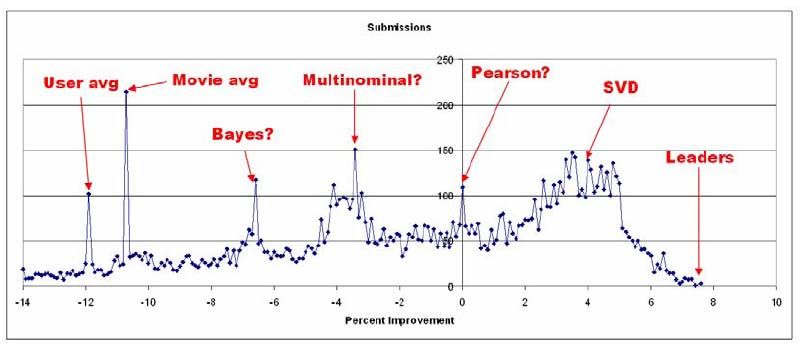
does a lot more than just optimize for RMSE. Figure 2 shows the distribution of the
leading submissions. Additional spikes with putative techniques, according to comments
made on the Netflix Prize Forum are also shown. These include the per-movie average
and the per-user average rating [1]. As it can be seen in the figure, most widely used
algorithms include Pearson correlation, Bayes, user average, movie average, SVD and
multidimensional algorithms. Our approach to this problem involves test & trial approach
where we first test a few simple approaches and progress to more advanced ones, and
report the findings.
Figure 2 Detail of distribution of leading submissions indicating possible techniques
In the following sections, we will describe the main methods we used for predicting
movies in Netflix dataset. As we already mentioned, we applied a number of different
methods such as simple average, double average, nearest neighborhood coupled with
background information, matrix factorization and slope one method. Some of these
methods achieved better results than other and some of them while working well, were
not able to do well on a large dataset such as Netflix due to resource constraints.
Following sections provide a detailed description of each used method.
Averaging Method
The most primitive approach will be to predict the rating of a movie for a user based on
average statistics. One can take different directions in this regard; for example one
method would be to assign average rate (3.8) to all movies for all users which we call as
simple average (see
Figure 3). The other method would be to calculate averages of movies for each user and
for that particular user to assign unrated movies as the calculated average rate which we
call as user average. Yet another method is to calculate averages over all users for anyspecific movies and then assign it in unrated cases, we call this later method as movie
average.
Figure 3 Rating Distribiutions1
The figure 3 shows the train and the probe set and rating distributions on them. These
above methods provide different RMSE values based on granularity and complexity of
taken approach. The following table 1 shows RMSE for each method.
Table 1 Averaging methods
Method RMSE
Simple average 1.13
Movie based average 1.05
User based average 1.017
Matrix factorization Method
One intuitive way to think of the Netflix data is as a matrix with rows corresponding to
users and columns corresponding to movies where it only has ratings for approximately
1% of the elements. One of the most successful and widely used approaches for
predicting these unknown ratings is Singular Value Decomposition (SVD) which
sometimes in information retrieval literature is referred to as LSI (Latent Semantic
1
Plot adopted from the following source: http://www.philbrierley.com/netflix/scoredist.gifIndexing). SVD methods are a direct consequence of a theorem in linear algebra which says that any m × n matrix A whose number of rows m is greater than or equal to its number of columns n, can be written as the product of an m × m column-orthogonal matrix U, and m × n diagonal matrix W with positive or zero elements (singular values), and the transpose of an n × n orthogonal matrix V as: A = UWV T More intuitively, assuming that we have an m × n matrix with m users and n movies; the theorem simply states that we can decompose such a matrix into three components: (m × m) call it U, (m × n) call it W, and (n × n) call it V. More importantly, we can use this decomposition to approximate the original m × n matrix. By taking the first k eigenvalues of the matrix W, we can effectively obtain a compressed representation. This approach shows the basic idea taken in SVD method. There are a variety of SVD implementation’s depending on the way it handles missing values and depending on its efficiency compromises, for example, JAMA package is a Java based matrix package that implements SVD. In addition to matrix based packages, there are also a number of standalone open source classes written in different languages such as the one that we are using in current project which is written in C++, based on [4]. Current SVD method assumes that a user's rating of a movie is composed of a sum of preferences about n aspects of that movie and correspondingly each user is described by n values describing how much they prefer each aspect. To combine these all together into a rating, each user preference is multiplied by the corresponding movie aspect, and then those n leanings add up into a final opinion of how much that user likes that movie. In matrix terms, the original matrix has been decomposed into two very oblong. Multiplying those together just performs the products and sums described above, resulting in approximation to the original rating matrix. By using singular value decomposition method we can find those two smaller matrices which minimize the resulting approximation error. The following equations show how error and aspects can be calculated. U [user ] = α ∗ e ∗ M [movie] M [movie] = α ∗ e ∗ U [user ] e = α ∗ (r − rpred ) The above conditions are evaluated for each rating in the training database where α is the learning rate, e is the residual error from the current prediction , r is actual rate and rpred is predicted rate for pair and M and U represent movie and user aspect matrixes. Using above equations, one feature (aspect) can be trained by finding the most prominent feature that will most reduce the error. After it does not show any more significant change, a new feature is started. To initialize rpred, one can use average movie ratings and to be more accurate, deviations can also be taken into account such that if Ra and Va are the mean and variance of all of the movies' average ratings and Vb is the average variance of individual movie ratings, then a bogus mean µ can be defined as in
following where r is any observed rating and µe is enhanced mean, note that 3.8 is
average global rating:

       n

     ∑r
μ=     r

       n
     Vb
k=
     Va
                  n
       3 .8 ∗ K + ∑ r
μe =              r

           K +n

Another tweak to current method is made possible by changing linear summation in
formula (1) into a non-linear function, G. One choice for G is to use a sigmoid function.
The next question is how to adapt G to the data, one straight forward way is to simply fit
a piecewise linear approximation to the true output/output curve.

Settings for this algorithm are mentioned in the following table for two different
experiments where we changed K in second experiment from 0.015 to 0.010, by using
these settings, we found an RMSE of 0.9260 on Netflix dataset:
                            Table 4. Parameters used in this experiment.

                        Parameter              Experiment I         Experiment II
                       Max features                  64                  64
                        Min Epochs                  120                  120
                        Max epochs                  200                  200
                      Min improvement             0.0001               0.0001
                       Learning rate               0.001               0.001
                             K                     0.015                0.010
                           RMSE                   0.9260               1.0006

Nearest Neighborhood Method
We also did prototype KNN approach and were curious to compare its performance. In
the Netflix problem, the goal is when given a set of training data user (u), movie (m),
time (t), rating (r), consisting of a sample of prior movie ratings r (an integer from 1 to 5),
associated with user (u), movie (m), time (t) to be able to accurately predict the rating that
should be associated with a new point [user (u), movie (m)]. In the analysis we will
ignore the time dimension for analysis. This approach was just a basic approach tried out!

For this experiment we decided to reduce the dataset size. The training data set provided
by Netflix was huge. If we were to run our algorithms on that dataset, we would lose a
significant amount of time waiting for the training to happen, especially with KNN
method. This would impair our ability to test small changes quickly. Therefore we
created training sets that are 1000, 100 and 10 times smaller (meaning they have so many
times fewer users), along with their respective testing sets. For this 5 different datasets
were created, by randomly selecting users.
This approach is based on movie similarity; we use the ratings given for a movie and by
the users and use the Euclidian distance as the similarity measure. We know that this
function of similarity treats all attributes similarly and this is a know weakness of KNN
and this can be eliminated by using weighted techniques. Given p and q are two points
and we can calculate the Euclidian distance using the given equation.
The advantage of this method is its online and though relatively simple, it’s
computationally intensive and in the past it performed well on similar recommendation
system problems. The KNN approach is a simple approach based on relative distance [8].
The observations using this approach are reported in the tables
We see that the only issue with KNN is that it requires all the training data to be present
in the order to make predictions and having a huge dataset is never a issue with the
memory but is an issue with time as we see that we need to compare it to all the items
which we are trying to make a prediction and this process may be very slow based on the
application. Another issue is finding the correct scaling factor, which turns out to be
tedious. Table 3 helps us look into identifying as how the variations of the k value would
help the RMSE to swing! We see that k=30 has an average RMSE of 1.09885 on a
fraction of the test set and when we use the similar approach on the entire test set we
would result in value ranges with approximately similar distributions [13].
Figure 4. Illustrating RMSE values for KNN from table 3Table 3. RMSE values across various K values
TRAIN SET Training K=1 k=3 k=5 k=10 k=30 k=100
1 1742 1.6024 1.3002 1.2436 1.1743 1.1476 1.1258
2 1742 1.4344 1.1979 1.1551 1.1339 1.1191 1.1069
3 1742 1.4374 1.182 1.1432 1.1497 1.1096 1.1179
4 1742 1.3872 1.1938 1.1928 1.1518 1.11 1.1128
5 1742 1.619 1.3091 1.2431 1.1684 1.1161 1.1118
Average 1.49188 1.24071 1.20657 1.15745 1.09885 1.10841
We also implemented the KNN approach using Euclidean measure for similarity using c#
classes but this was not optimized for time and memory. This was taking tedious amount
of time for basic runs and the first simple approach for trying to look at variations of k
was done using the simple KNN approach using. Some future directions to this work
include using other similarity measures such as Pearson’s coefficient, and cosine based
similarity.
Slope One Method
Slope one is a family of algorithms used for Collaborative filtering [2]. Arguably, it is the
simplest form of non-trivial item-based collaborative filtering based on ratings. Its
simplicity makes it especially easy to implement while its accuracy is often on par with
more complicated and expensive algorithms [2]. The algorithm itself is based on the idea
of a “popularity differential” between items. For example, if User A rates Item J 0.5 stars
higher than Item I, then User B might also like Item J by about 0.5 stars more than Item I.
This is demonstrated in Figure 5.
Figure 5 The Slope One algorithm ideaThe name of the algorithm, slope one, derives from the fact that we are essentially estimating an equation of the form f(x) = x + b, where f(x) is the prediction and x is an average of ratings for a training movie. We estimate b for many different training movies, and combine the results of the functions to get a prediction. Functions with additional coefficients, like f(x) = ax + b or f(x) = ax2 + bx + c may be used, but previous work has shown no significant increase in performance over f(x) = x + b [2]. Formally, P(u) is defined as a prediction vector, where each component P(u)i is the contribution that one item in the training set, item i, makes to the prediction. We are predicting on item j. Rj is the set of relevant items, i.e. the items other than j that the user has rated, and card(Rj) is the size of the set Rj. Let ui be the rating that the user gave item i. Define devj,i to be the average difference between the ratings for items i and j across all users who have rated both i and j. Then, the Slope One algorithm can be summarized as follows: This defines the value of each component of the prediction vector. To get the overall prediction, it’s also possible to do a weighted average of the components, either with equal weights for standard slope one, or with different weights for weighted slope one. This version takes into account the number of users who rated a specific item in Rj. If more users rated an item, the accuracy of that component of the prediction is assumed to be greater, so it is weighted more heavily. The weights increase linearly with the number of users who rated the item. So, for each component of the prediction vector P(u), there is an associated weight value contained in the vector W(u), where each entry is the number of users rating both the predictee item and the training item. The overall prediction P is then: Regarding time and space complexity, suppose that there are n items and m users. Computing the average rating differences for each pair of items requires up to n2 units of storage, and up to m n2 time steps. Considering the fact that n2 in our problem is too large to be handled in a conventional size memory and also regarding the fact that Java memory allocation is not efficient (especially for dynamic objects which are created on the heap), we were not able to hold the entire dataset in memory. Rather we decided to run on top 50 most frequently rated movies and substitute missing predictions by 3.8 which is the average rate, this resulted in an RMSE of 1.1335. This result is very close to random result (1.1357) due to small number of training files (top 50 most frequently rated movies). It can be improved in several different ways, by increasing number of files, running it on a more powerful machine, using C++ instead of Java to avoid inefficient memory allocation of Java, and using a stratification method to combine results from different size sets.
Additional Methods and Approaches
Additional methods such as decision trees, neural networks, and other such learning
techniques would work on the dataset and would produce some results, but when the
problem is approached it logically appears to be a relational problem and relational
learning techniques best suite this problem. We should also remember that the learning
tools such as Weka, Taste, Rapid Miner (YALE) and more, would not be suitable tools as
they give memory and computational constraints as well as not all of them are equipped
with learning classifiers which would be best suitable for this problem. We observe that
methods such as clustering by k-means [9], support vector regression [10], and time
series models can be some other approaches which can be experimented with and would
have promising results. An ensemble formed using above methods might serve as a future
winner in this recommendation system contest.

One major problem would be handling the missing values, which still would be
challenging, if the userid or movieid where missing, adding a new user or an old user or a
new movie or a old movie would make the whole process as an approximation and
would make it heuristically biased. But if given a userid and movieid and if we have the
user rating missing then we can use clustering or a weighted approach to fill this missing
value and continue the analysis and see if this helps the experimentation or not.

Conclusion
Advanced methods including, the SVD, were the apple’s eye. Among all the experiments,
SVD does a better job which results in a RMSE of 0.9260 on the Netflix dataset and
stands as over niche technique for this project. The figure 6 compares different RMSE
values from different algorithms used in current project. The KNN based
recommendation systems are more popular systems in this domain, but due to our current
time, memory and resources constraints, proper data conditioning and analysis would
take a longer time and many not be feasible to reach very good results, and thus it was
included as a prototype model.

One clear idea in mind was to extend the KNN based approach using clustering in
preprocessing where we have a better data conditioning, where we increase the attribute
or dimensionality and then apply clustering to include user based information and later
apply item based collaborative filtering for enhanced performance. Also SVD methods
are extremely computationally efficient, requiring only an inner product and the solution of a
low-dimensional linear system and are capable in a way address bias via posterior bias
correction techniques. For this SVD specifically we include specific customer bias and movie
based bias and the future work can include ways to remove this for better results. In KNN the
value of K helps to formulate the bias for the overall model, thus K should always be set to
such a value that it should always minimize the probability of misclassification. Defining the
degree of bias for these algorithms is very challenging and our discussions point to the most
general bias issues.
Some of the future work includes experimenting using ensemble made of a combination
of these techniques. Also we can evaluate support vector regression machines for
prediction. Another approach can involve time and take time of movie release, and the
movie ratings from IMDB [12] and the time of the release of DVD and other such similar
or related attributes involving time and apply time series based regression models [11]
and evaluate the prediction accuracy.

                        Figure 6 Comparing best RMSE of different methods.

On November 13, 2007, the team KorBell (also known as BellKor) had been officially
declared the winner of the $50,000 Progress Prize [7] with their RMSE of 0.8712 (8.43%
improvement). In order to win the 2008 Progress Prize, one should obtain the RMSE of
0.8625 or better on the quiz set [5].

References
1.  The Netflix Prize, James Bennet, Stan Lanning, in Proceedings of KDD Cup and Workshop 2007, San
    Jose, California, 2007
2. Daniel Lemire, Anna Maclachlan, Slope One Predictors for Online Rating-Based Collaborative
    Filtering, In SIAM Data Mining (SDM'05), Newport Beach, California, April 21-23, 2005.
    http://www.daniellemire.com/fr/documents/publications/lemiremaclachlan_sdm05.pdf
3. The Netflix Prize Dataset. Netflix, Inc. http://www.netflixprize.com/
4. Netflix Update: Try This at Home, http://sifter.org/~simon/journal/20061211.html. , last update
    December 2006.
5. http://en.wikipedia.org/wiki/Netflix_Prize Retrieved: December 10, 2007.
6. Plot adopted from the following source: http://www.igvita.com/blog/2006/10/29/dissecting-the-netflix-
    dataset/
7. http://www.netflixprize.com/leaderboard
8. http://en.wikipedia.org/wiki/Nearest_neighbor_(pattern_recognition) retrieved December 9, 2007
9. http://dmnewbie.blogspot.com/2007/08/great-collaborative-filtering_29.html retrieved December 9,
    2007.
10. http://www.svms.org/regression/ retrieved December 9, 2007.
11. http://en.wikipedia.org/wiki/Autoregressive_integrated_moving_average retrieved on December 9,
2007.
12. http://imdb.com/ retrieved on December 10,2007.
13. http://www.erikshelley.com/netflix/ retrieved on december 10, 2007.You can also read