Optimal Image-Based Guidance of Mobile Manipulators using Direct Visual Servoing
←
→
Page content transcription
If your browser does not render page correctly, please read the page content below
Article
Optimal Image-Based Guidance of Mobile
Manipulators using Direct Visual Servoing
Álvaro Belmonte, José L. Ramón, Jorge Pomares *, Gabriel J. Garcia and Carlos A. Jara
 Dpt of Physics, Systems Engineering and Signal Theory, University of Alicante, Alacante, Spain;
 bb35@alu.ua.es (A.B.); jl.ramon@ua.es (J.L.R.); gjgg@ua.es (G.J.G.); carlos.jara@ua.es (C.A.J.)
 * Correspondence: jpomares@ua.es; Tel.: +34 965903400

 Received: 20 February 2019; Accepted: 23 March 2019; Published: 27 March 2019

 Abstract: This paper presents a direct image-based controller to perform the guidance of a mobile
 manipulator using image-based control. An eye-in-hand camera is employed to perform the
 guidance of a mobile differential platform with a seven degrees-of-freedom robot arm. The
 presented approach is based on an optimal control framework and it is employed to control mobile
 manipulators during the tracking of image trajectories taking into account robot dynamics. The
 direct approach allows us to take both the manipulator and base dynamics into account. The
 proposed image-based controllers consider the optimization of the motor signals sent to the mobile
 manipulator during the tracking of image trajectories by minimizing the control force and torque.
 As the results show, the proposed direct visual servoing system uses the eye-in-hand camera
 images for concurrently controlling both the base platform and robot arm. The use of the optimal
 framework allows us to derive different visual controllers with different dynamical behaviors
 during the tracking of image trajectories.

 Keywords: visual servoing; optimal control; mobile manipulator; dynamic control

1. Introduction
      This paper proposes a direct image-based visual servoing system for the guidance of a mobile
manipulator. As described throughout the paper, the visual information is employed to guide both
the robot manipulator and the base platform for the tracking of image trajectories. A common
classification for visual servoing systems based on position and image is established [1]. Within the
field of position-based visual servoing systems, it is worth mentioning some classic works [2] as well
as some more recent ones such as the works of Huang et al. [3]. Besides these two works, it is worth
mentioning other remarkable ones such as the works of Park et al. [4], which describes the use of
vision for a robot’s positioning with regard to an object whose position was previously determined.
Position-based systems are those where the reference of the control system is in a desired
tridimensional position and orientation. In contrast to position-based approaches, image-based
visual servoing systems determine the reference in the image space. This strategy is the one used in
this paper. Although the literature regarding image-based visual servoing is quite extensive, works,
such as the presented in [1,5], perform a review of the classical approaches and problems related to
indirect image-based controllers. One of the elements which most affects the behavior of
image-based visual servoing controllers is the interaction matrix, which is employed by the
controller and depends on several parameters. The interaction matrix J is employed by the
image-based visual servoing controllers for relating velocities in a tridimensional point with
velocities of a corresponding point in the image space. Deep learning approaches are currently in
development for image-based control of robot manipulators (see e.g. [6,7]). When this kind of
approaches has to be applied to a mobile manipulator, it is necessary to consider not only the
manipulator but also the mobile platform, having a redundant system. When dealing with stability

Electronics 2019, 8, 374; doi:10.3390/electronics8040374                      www.mdpi.com/journal/electronics
Electronics 2019, 8, 374 2 of 13
problems, it is worth mentioning those that stem from dealing with a redundant robot [8]. In this
case, it is not only necessary to correctly perform the end effector guidance, but also to solve the
redundancy by establishing the most appropriate joint configuration for each situation.
Another useful classification depending on the control strategy of visual servoing systems
divides them in direct and indirect visual servoing. In indirect visual servoing, the control action is
specified as velocities to be applied at the robot’s end effector and does not take robot dynamics into
account. In this case, the internal robot controller is used and translates these velocities into torques
and forces for the joints. When applying an indirect controller to a task only kinematic aspects of the
robot are taken into account. However, in direct controllers, the control action is usually given as
forces and torques applied directly to the manipulator joints. By using this approach, the internal
feedback control loop for the servomotors is removed, and the visual information is used to directly
generate the currents or torques to be applied to the motors of the robot’s every joint. Some direct
visual control systems for redundant robots with chaos compensation have been developed to avoid
robotic chaotic behaviors with new architectures to improve systems maintainability and traceability
[9,10]. Within the field of direct image-based visual servoing systems it is worth mentioning works
such as [11] that considers a FPGA (Field Programmable Gate Arrays) implementation, or [12] that
extends the previous direct visual servoing for the optimal control of robot manipulators.
Within the field of indirect visual servoing, several approaches can be found for the guidance of
mobile robots or mobile manipulators. In [13], a homography-based 2D approach for visual control
of a mobile manipulator that does not need any measure of the 3D structure of the observed target
has been proposed. A task-space sensing and control system designed to control the end effector
motion of a mobile manipulator in the presence of dynamic and unknown base motion is proposed
in [14]. In [15], an image-based approach with redundancy resolution is proposed for the guidance
of a mobile manipulator. An indirect position-based visual control approach is described in [16] for
the guidance of a mobile manipulator. In [17], a control scheme that uses image-based visual
servoing was developed along with a functional mobile manipulator platform, where a hybrid
camera configuration composed of monocular and stereo vision cameras was integrated into the
system.
In contrast with previous approaches, the one proposed in this paper employs a direct visual
servoing system for guiding mobile manipulators. In this case, the controller directly generates the
torques, forces, and moments to be applied to the manipulator and base platform taking into account
the robot dynamics. In the previous indirect approaches, the controller assumes that the guided
device is a perfect positioning system, and therefore its dynamics is not considered. However, the
use of a direct visual servo approach allows for the manipulator and base dynamics to be taken into
account. The result is a faster and more accurate control that reacts more quickly to abrupt changes
in the image trajectories. Additionally, an optimal control approach is used for the definition of the
proposed controllers. This control approach considers the optimization of the motor signals sent to
the mobile manipulator during the tracking of image trajectories. Using this optimal approach,
different visual controllers with different dynamic properties can be derived.
The paper is divided into the following sections. First, Section 2 describes the robotic system
and main coordinate frames. The system kinematics is described in Section 3 and the dynamics in
Section 4. Section 5 describes the optimal controller and the visual servoing of the mobile
manipulator. Finally, in Section 6, the main results obtained in the application of the proposed
optimal controller are described.
2. System Architecture and Nomenclature
Figure 1 represents the main components of the mobile manipulator (TIAGo robot from PAL
Robotics). The robot is composed of a mobile differential platform with a 7-DOF
(degrees-of-freedom) arm, a RGB-D camera which is not employed in this paper, and an additional
eye-in-hand camera. Frame ℱ is attached to the mobile robot platform and ℱ is the manipulator
arm coordinate system attached to the base of the robot arm. The origin of ℱ is translated with
respect to the frame ℱ a vector ( , , ). The world coordinate frame is called ℱ . The endElectronics 2019, 8, 374 3 of 13
effector frame ℱ is attached to the manipulator end effector, and frame ℱ is the eye-in-hand
camera frame. In this paper we consider an eye-in-hand camera system where ℱ = ℱ . The
orientation of the mobile platform is considered as α, i.e., the angle between de X-axis of the frame
ℱ and the X-axis of the frame ℱ and the origin of ℱ is at the position ( , , ) with respect to
ℱ . From the manipulator kinematics we can obtain the position of ℱ with respect to ℱ as
( , , ) and ( , , ), respectively.
Regarding the visual system, an eye-in-hand camera observes a set of four visual features
located on the surface of the tracked object. As Figure 1 shows, a black pattern with four white points
is located in the tracked object. Therefore, the computer vision extracts four visual feature points,
T
= , , , , that correspond to the center of these white points. Figure 2 shows the different
modules that compose the computer vision system. The first step preprocesses the image in order to
obtain a single format of the image no matter what camera is employed (e.g., image conversion from
RGB to gray scale, image resizing, noise filtering, etc.). In the second stage, the image is binarized
through a thresholding process. The result is a binary image with all the essential data of the pattern.
The third step is an erosion operation. This is a morphological operation on the image that removes
the pixels located on the edge of any object in the image. This step is mainly used to reduce the noise
of the image. The fourth phase is the most important stage of the vision module: blob detection. The
purpose of this module is to detect the connected pixels which form an object in the image and then
assign a label to them. Finally, the vision module has to provide the pixel coordinates of the center of
gravity of the visual features. The fifth submodule (area and centroid computation) accomplishes
this task. In [12], a detailed description of the computer vision components required to determine the
set of visual features is presented.
Figure 1. System components.
Figure 2. Computer vision components.
3. System Kinematics
The main components and coordinate frames of the robotic system are presented in Section 2.
This section describes the kinematic formulation required for the definition of the proposed
controllers. ∈ ℜm represent the generalized joint coordinates of the manipulator (in our case, mElectronics 2019, 8, 374 4 of 13
= 7) and ∈ ℜnp are the generalized coordinates of the platform. The generalized coordinates of
both manipulator and platform can be represented as = . In a general case, the computer
T
vision system extracts k visual feature points from the observed object = , ,…, ∈ ℝk (k = 4
in the experiments, see Figure 1). Therefore, the image-based direct visual controller must perform
the guidance of the mobile manipulator to track the desired trajectory in the image space, sd(t). The
visual servoing control approach allows the control of the manipulator joints and base using k visual
features, using an eye-in-hand configuration, where a camera is held by the end effector.
Considering an image feature point, , , the relationship between velocities in the camera image
space, ̇ , and the velocity twist ṙ c = [ ] of the camera (expressed in its own frame), is given
by:
̇ = J ,, (1)
where is the depth of the image feature and the value of J can be found in [1]. From a kinematic
point of view, the motor commands are considered as a set of platform command velocities, ∈
ℝp , and manipulator command velocities, ∈ ℝm , therefore
= (2)
In the above equation the manipulator motor commands are the joint velocities, i.e., ̇ = ,
and from the kinematic model of the mobile platform the following relation can be considered:
̇ =
(3)
where, usually, =[ ] is the platform linear and angular velocities and the function
spans the admissible velocity space at each mobile platform configuration. In this paper, an
image-based approach will be employed for the guidance of the mobile manipulator, therefore, an
image Jacobian, J , must be defined which relates the differential mapping between the motor
commands and the time derivative of the set of image features s:
̇ =J
(4)
where J will be defined throughout the paper as the product of the matrices J and J , therefore,
J = J J . The interaction matrix J ∈ ℝ2k×6 for the set of image features points, s, is the stack of k
matrices J for each feature:
J ( , )
̇ =J ( , ) = ⋮ (5)
J ( , )
where = [ … ] ∈ ℝk is a depth vector for each image feature. The matrix J relates the
end effector velocity with respect to the camera coordinate frame [ ] and the motor
command :
=J ( ) (6)
As previously described, the mobile manipulator is composed of a differential drive platform
and a 7-DOF robot arm with an eye-in-hand camera. In order to derive the value of the matrix J ,
first the position and orientation of the camera with respect to the world coordinate ℱ is defined as
=[ ( ) ( )] = [ ]
(7)
where ( ) represents the position and ( ) is the minimal parametrization of the camera
orientation by Euler angles. From the robot kinematics and the system architecture presented in
Section 2, it is possible to obtain
= + − + +
(8)
= + + + +
(9)Electronics 2019, 8, 374 5 of 13
= +
(10)
From the previous equations we can obtain the time derivatives of , i.e., [ ] . First, the
components of the translation velocity, ̇ ( ), can be defined as
̇ = ̇ − + ( ) − ̇ − + ( ) +
(11)
̇ = ̇ + + ( ) + ̇ − + ( ) +
(12)
̇ = ̇
(13)
Therefore, the motion of the manipulator end depends not only on the joint positions and
velocities of the manipulator arm but also on the motion of the mobile platform and its orientation
. Additionally, the components of the angular speed, ̇ ( ) of the robot can be computed as [15]
̇ = ̇ − ̇
(14)
̇ = ̇ − ̇
(15)
̇ = ̇ +
(16)
From Equations (11)–(16) the values of [ ] = ̇ ̇ ̇ ̇ ̇ ̇ are obtained
with respect to the motor commands. Using the rotation matrix R , which represents the orientation
frame ℱ with respect to ℱ , the values of [ ] can be expressed with respect to the frame ℱ ,
[ ] . Appendix A describes the computation of the numerical values of matrix J .
Another useful kinematic relationship for the definition of the proposed controllers is the image
acceleration or second time derivative of s. This relationship is obtained by the definition of J
(Equation (4)) and differentiating w.r.t.
̈ =J ̇ + ̇
(17)
4. System Dynamics
This section describes the main dynamic equations for the robotic system. The dynamic
equations of motion of the mobile manipulator can be written as
F M M ̇
= T + (18)
M M ̈
where ̈ ∈ ℜm is the set of joint accelerations of the robot manipulator, ̇ = [ ̇ ̇ ] is the
platform linear and angular accelerations, M ∈ ℜ × is the inertia matrix of the platform,
M ∈ ℜ × is the coupled inertia matrix of the base and the manipulator, and M ∈ ℜ × is
the inertia matrix of the manipulator; and are a velocity/displacement-dependent, nonlinear
terms for the base and manipulator, respectively, F is the force and moment exerted on the base,
and is the applied joint torque on the robot manipulator. From a dynamic point of view, the
motion of the mobile manipulator is governed by the applied torques on the manipulator joints and
by the force and moment exerted on the base. Hence, Equation (18) can be written in the following
compact form.
=M ̇ +C
(19)
F M M ̇
where = , M= , ̇ = , and C = .
MT M ̈Electronics 2019, 8, 374 6 of 13
5. Optimal Control of the Mobile Manipulator
5.1. Optimal Control Definition
In complex high dimensional systems, several tasks can be accomplished simultaneously taking
advantage of the robot redundancy. This paper considers a system with µ constrains that represents
the task for the mobile manipulator to be executed. These constraints can be represented as
A(t) ̇ = b(t) (20)
where A(t) ∈ ℜµ×(p+m) and b(t) ∈ ℜµ×1 . An advantage of this task formulation is that
nonholonomic constraints can be treated in the same general way. In order to reduce the energy
required for performing the visual servoing task, the proposed optimal controller is designed to
minimize the control torque for the mobile manipulator, considering the following cost function.
Ω(t) = T W(t)
(21)
where W(t) is a time-dependent weight matrix.
Let us assume that the robot model presented in the previous section and a constraint
formulation are given. In this case, the optimal controller has to guarantee that the task is perfectly
achieved, i.e., that A(t) ̇ = b(t) holds at all times. Additionally, the minimization of the control
command with respect to some given metric, i.e., Ω(t) = T W(t) , is intended at each instant of time.
The solution to this pointwise optimal control problem [18] can be derived from a generalization of
Gauss’ principle, as originally suggested in [19]. It is also a generalization of the propositions in
[20,21], where the following control action is obtained considering the general expression for the
dynamic model expressed in Equation (19) (for the sake of clarity the time dependences are not
indicated):
-1 + -1
= W-1/2 AM W-1/2 · b + AM C (22)
where the symbol + denotes the pseudo inverse of a general matrix. As it can be seen in Equation
(22), the matrix W is an important factor in the control law that can be used to determine how the
control efforts are distributed over the joints and the robot base.
5.2. Optimal Direct Visual Servoing
Once the optimal control framework is presented in Section 5.1, this section describes its
application for the optimal control of the mobile platform. First, we define s̈ r as the reference image
accelerations that will be employed by the optimal controller. The value of these image accelerations
can be obtained from Equation (17). This last expression can be expressed into the form of Equation
(20) as
J ̇ = ̈ − ̇
(23)
This way, the visual servoing task is defined by the following relationships.
A=J
(24)
= ̈ − ̇
Therefore, with the given definition of A and b, the optimal control will minimize the motor
commands while performing the tracking in the image space. The final control law can be obtained
replacing these variables into the function that minimizes the motor signals described by Equation
(22):
-1 + -1
= W-1/2 J M W-1/2 · ̈ − ̇ +J M C (25)
As it can be seen, the visual controller represented by (25) implicitly depends on the weighting
matrix W, and different values of this matrix can be used to coordinate the motion of the base and of
the manipulator. The diagram of the considered control loop is depicted in Figure 3.Electronics 2019, 8, 374 7 of 13
Robot Kinematics and Dynamics
J , M, C
Desired trajectory ̈ Optimal
K ,K ROBOT
̈ , ̇ , controller W
̇ ̈
Visual feedback ̇,
Figure 3. Diagram of the control scheme for the mobile manipulator robot.
-2
Considering =M and replacing this value in the control framework expressed in Equation
(25), the result yields
-1
=M · ̈ − ̇ +J M C (26)
This controller represents a direct visual servo control using inversion of the dynamic model.
Additionally, new controllers can be obtained using different values of W. For example, an
-1
important value for W, due to its physical interpretation, is = M , since it is consistent with the
principle of d’Alembert:
1/2 -1 1/2 + -1
=M JM M · ̈ − ̇ +J M C (27)
Now, the definition of the reference control, s̈ r , is described considering the eye-in-hand
camera system that extracts a set of k image feature points. The task description as a constraint is
given by the following equation in the image space.
( ̈ − ̈) + K ( ̇ − ̇) + K ( − ) = 0
(28)
where ̈ , ̇ , and are the desired image space accelerations, velocities, and positions,
respectively. K and K are proportional and derivative gain matrices, respectively. This equation
can be expressed in regards to image error in the following way.
̈ +K ̇ +K = ̈
(29)
where and ̇ are the image error and the time derivative of the image error, respectively. As
stated, the variable ̈ denotes the reference image accelerations of the proposed image space based
controller. Substituting this variable into the dynamic visual servo controller in Equation (25), the
control law is set by the following relationship.
-1 + -1
= W-1/2 J M W-1/2 · ̈ +K ̇ +K − ̇ +J M C (30)
In order to demonstrate the asymptotic tracking of the control law, some operations must be
done. First, the closed-loop behavior is computed from Equation (19) as
-1 + -1
M ̇ + C = W-1/2 J M W-1/2 · ̈ +K ̇ +K − ̇ +J M C (31)
-1
Equation (31) can be simplified by premultiplying its left and right sides by J M W-1/2 W1/2 :
J ̇ = ̈ +K ̇ +K − ̇
(32)
Finally, using the relationship expressed in (23), it can be concluded that
̈ =− K ̇ − K
(33)
Therefore, when J is full-rank, an asymptotic tracking is achieved by the visual servo
controller expressed in Equation (30) for the tracking of an image trajectory.Electronics 2019, 8, 374 8 of 13
6. Results
This section presents the system behavior during the tracking of different trajectories. The robot
is guided by an eye-in-hand camera system. The parameters of a Gigabit Ethernet TM6740GEV
camera is considered, which acquires 200 images every second with a resolution of 1280 × 1024
pixels. The eye-in-hand camera extracts four visual features from the four corners of the target.
Three different experiments are presented in this section. In these experiments the value of W =
M−1 is considered. Figure 4a,b represents the initial configuration employed in all of the experiments.
Figure 4a represents the target and the mobile manipulator with the eye-in-hand camera system. The
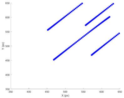
initial position of the visual features is represented in Figure 4b. The desired trajectory employed in
the first experiment is a linear trajectory that represents a lateral translation of 200 px. in x and y
directions in the image from the initial position of the visual features. As it can be seen in Figure 4d,
the image-based controller correctly carries out the tracking and a straight line is obtained in the
image space. Figure 4c represents the final pose of the mobile manipulator. The second experiment,
represented in Figure 4e,f, evaluates the tracking when a displacement in depth must be performed.
As it can be seen in Figure 4e, a displacement in depth is carried out and, once the experiment ends,
the mobile manipulator is closer to the target. Figure 4f represents the obtained image trajectory.
This trajectory corresponds to the desired trajectory specified as a linear increase in depth from the
initial image configuration. Finally, the experiment represented in Figure 4g,h requires a change in
orientation of the eye-in-hand camera with respect to the observed target. To do this, the desired
image trajectories for the visual features are represented by a straight line between the initial and the
T
final ones defined as ∗ = = (503, 584), = (612, 600), = (523, 472), = (630, 477)
px. As in the previous experiments, Figure 4g represents the final robot pose once the experiment
ends and Figure 4h represents the image trajectory. As the experiments show, the proposed
controller allows the concurrent guidance of both the manipulator and robotic platform during the
tracking of the desired image trajectory.
Figure 5 represents the joint torques applied to the manipulator (m = 1…7) and force and
moments applied to the robot platform during the first and second experiments. As it can be seen in
Figure 5a (first experiment), the torques, force, and moment remain low, and a smooth behavior is
obtained during the tracking. For the second experiment, Figure 5b represent the joint torques
applied to the manipulator and force and moment applied to the base platform during the robot
motion in depth. It is worth noting that the reduction of the distance between the two bodies (target
and robot) is obtained by modifying both the base platform pose and the robot manipulator joint
configuration. Finally, as in the previous experiments, Figure 6 represents the joint torques applied
to the manipulator and force and moment applied to the base platform during the third tracking
experiment. The desired relative orientation is achieved by controlling both the orientation of the
base platform and the robot manipulator joint configuration.Electronics 2019, 8, 374 9 of 13
(a) (b)
(d)
(c)
(e) (f)
(g) (h)
Figure 4. Robot pose and image trajectories in the experiments. (a) 3D initial pose of the mobile
manipulator and target. (b) Initial visual features extracted by the eye-in-hand camera. FirstElectronics 2019, 8, 374 10 of 13
experiment: (c) 3D final pose. (d) Image trajectory. Second experiment: (e) 3D final pose. (f) Image
trajectory. Third experiment: (g) 3D Final pose. (h) Image trajectory.
(a) (b)
Figure 5. (a) Experiment 1: Joint torque and moment and force exerted on the base platform. (b)
Experiment 2: Joint torque, moment, and force exerted on the base platform.
)
Figure 6. Experiment 3: Joint torque, moment, and force exerted on the base platform.
One of the main advantages of the proposed controller is the possibility to define new direct
image-based controllers by modifying the value of the matrix W of the optimal controller (see
Equation (25)). A different controller with different dynamic behavior during the tracking of image
trajectories can be obtained by modifying this matrix. In order to evaluate the proposed framework,
in Table 1 we represent the obtained image error during the tracking of a repetitive image trajectory
defined by the following equation.
320 + 166 ( + ⁄4)
= = (34)
265 + 160 ( + ⁄4)
Table 1 represents the mean error in pixels and mm during the tracking of the image trajectory
considering different tracking velocities. As it can be seen in this table, different tracking errors are
-1
obtained and the best behavior at high velocities is obtained considering = M . Additionally, theElectronics 2019, 8, 374 11 of 13
performance of the controllers is compared with respect to previous controllers only based on
inverse dynamics [22] (indicated as “previous” in Table 1).
Table 1. Mean image error in pixels (mm) during the tracking of the image trajectory.
= 0.5 rad/s = 1 rad/s = 2 rad/s
-2
=M 2.14 px (0.59 mm) 2.21 px (0.61 mm) 3.84 px (1.04 mm)
-1
=M 2.12 px (0.58 mm) 2.95 px (0.8 mm) 2.39 px (0.66 mm)
= 3.81 px (1.03 mm) 3.22 px (0.87 mm) 4.4 px (1.2 mm)
Previous 2.25 px (0.62 mm) 3.2 px 0.85 mm) 4.12 px (1.09 mm)
7. Conclusions
This paper presents a direct image-based visual servoing system for the guidance of mobile
manipulators. This approach is based on an optimal framework that considers the optimization of
the motor signals sent to the mobile manipulator during the tracking of image trajectories. The
stability of the controller has been proved analytically, and different dynamical behavior can be
obtained by using different values of the matrix W.
As a result, an adaptive and flexible tool has been obtained, allowing for concurrent control of
both the base platform and manipulator during the tracking of trajectories. With the given definition
of A and b, the optimal control can minimize the motor commands while performing the tracking of
trajectories in the image space. The viability of the controller has been tested in a variety of test case
experiments, including approaches to an object, as well as different positioning tasks that require
modifying the position and/or the orientation of the mobile manipulator. In all such cases, the
experiments and trajectories have been accomplished.
Author Contributions: Funding acquisition, C.A.J.; Methodology, J.L.R.; Software, Á.B.; Supervision, J.P.;
Validation, G.J.G.
Funding: This research was supported by the Valencia Regional Government through project GV/2018/050.
Conflicts of Interest: The authors declare no conflict of interest.
Appendix A
As described throughout the paper, the motor commands are = =[ ̇ ] .
First, the robot Jacobian is used to convert the joint velocities to Cartesian velocities:
⎡ ⎤
⎢ ̇ ⎥
⎢ ̇ ⎥
⎢ ⎥ × ×
⎢ ̇ ⎥= (A1)
× ×
⎢ ̇ ⎥
⎢ ̇ ⎥
⎢ ⎥
⎣ ̇ ⎦
The relation between the previous Cartesian velocities and [ ] can be obtained by using
Equations (11)–(16):
̇ ⎡ ⎤
⎡ ⎤ ⎢ ̇ ⎥
̇
⎢ ⎥ ⎢ ⎥
̇ ̇
⎢ ⎥ × ⎢ ⎥
⎢ ̇ ⎥= ⎢ ̇ ⎥ (A2)
× ̇
⎢ ⎥ ⎢ ⎥
̇ ⎢ ⎥
⎢ ⎥ ̇
⎣ ̇ ⎦ ⎢ ⎥
⎣ ̇ ⎦
Where,Electronics 2019, 8, 374 12 of 13
− − − 0 0 0 0
= + 0 0 0 0
0 0 0 0 1 0 0 0 (A3)
0 0 0 0 0 − 0
= 0 0 0 0 0 − 0
0 1 0 0 0 0 0 1
Finally, by using the rotation matrix R which represents the orientation frame ℱ with
respect to the fame ℱ , the values of [ ] can be expressed with respect to the frame ℱ ,
[ ] .
= (A4)
Therefore, the value of J is equal to
× × ×
J = (A5)
× × ×
References
1. Chaumette, F.; Hutchinson, S. Visual servo control. I. Basic approaches. IEEE Robot. Autom. Mag. 2006, 13,
82–90.
2. Allen, P.K.; Yoshimi, B.; Timcenko, A. Real-time visual servoing. In Proceedings of the 1991 IEEE
International Conference on Robotics and Automation, Sacramento, CA, USA, 9–11 April 1991; pp. 851–
856.
3. Huang, P.; Zhang, F.; Cai, J.; Wang, D.; Meng, Z.; Guo, J. Dexterous Tethered Space Robot: Design,
Measurement, Control, and Experiment. IEEE Trans. Aerosp. Electron. Syst. 2017, 53, 1452–1468.
4. Park, D.; Kwon, J.; Ha, I. Novel Position-Based Visual Servoing Approach to Robust Global Stability Under
Field-of-View Constraint. IEEE Trans. Ind. Electron. 2012, 59, 4735–4752.
5. Chaumette, F.; Hutchinson, S. Visual control. II. Advanced approaches. IEEE Robot. Autom. Mag. 2007, 14,
109–118.
6. Bateux, Q.; Marchand, E.; Leitner, J.; Chaumette, F.; Corke, P. Training Deep Neural Networks for Visual
Servoing. In Proceedings of the 2018 IEEE International Conference on Robotics and Automation (ICRA),
Brisbane, Australian, 21–25 May 2018; pp. 1–8.
7. Levine, S.; Pastor, P.; Krizhevsky, A.; Ibarz, J.; Quillen, D. Learning hand-eye coordination for robotic
grasping with deep learning and large-scale data collection. Int. J. Robot. Res. 2018, 37, 421–436.
8. Agravante, D.J.; Claudio, G.; Spindler, F.; Chaumette, F. Visual Servoing in an Optimization Framework for
the Whole-Body Control of Humanoid Robots. IEEE Robot. Autom. Lett. 2017, 2, 608–615.
9. Pomares, J.; Jara, C.A.; Perez, J.; Torres, F. Direct visual servoing framework based on optimal control for
redundant joint structures. Int. J. Precis. Eng. Manuf. 2015, 16, 267–274.
10. Pomares, J.; Perea, I.; Torres, F. Dynamic Visual Servoing With Chaos Control for Redundant Robots.
IEEE/ASME Trans. Mechatron. 2014, 19, 423–431.
11. Alabdo, A.; Pérez, J.; Garcia, G.J.; Pomares, J.; Torres, F. FPGA-based architecture for direct visual control
robotic systems. Mechatronics 2016, 39, 204–216.
12. Pérez, J.; Alabdo, A.; Pomares, J.; García, G.J.; Torres, F. FPGA-based visual control system using dynamic
perceptibility. Robot. Comput. Integr. Manuf. 2016, 41, 13–22.
13. Benhimane, S.; Malis, E. Homography-based 2D Visual Tracking and Servoing. Int. J. Robot. Res. 2007, 26,
661–676.
14. Sandy, T.; Buchli, J. Dynamically decoupling base and end-effector motion for mobile manipulation using
visual-inertial sensing. In Proceedings of the 2017 IEEE/RSJ International Conference on Intelligent Robots
and Systems (IROS), Vancouver, BC, Canada, 24–28 September 2017; pp. 6299–6306.
15. Luca, A.D.; Oriolo, G.; Giordano, P.R. Image-based visual servoing schemes for nonholonomic mobile
manipulators. Robotica 2007, 25, 131–145.
16. Lang, H.; Khan, M.T.; Tan, K.K. Application of visual servo control in autonomous mobile rescue robots.
Int. J. Comput. Commun. Control 2016, 11, 685–696.
17. Wang, Y.; Zhang, G.; Lang, H. A modified image-visual servo controller with hybrid camera configuration
for robust robotic grasping. Robot. Auton. Syst. 2014, 62,1398-1407.
18. Spong, M.; Thorp, J.; Kleinwaks, J. The control of robot manipulators with bounded input. IEEE Trans.
Autom. Control 1986, 31, 483–490.Electronics 2019, 8, 374 13 of 13
19. Udwadia, F.E. A new perspective on tracking control of nonlinear structural and mechanical systems. Proc.
R. Soc. Lond. Ser. A 2003, 1783–1800.
20. Udwadia, F.E.; Kalaba, R.E. Analytical Dynamics: A New Approach; Cambridge University Press: Cambridge,
UK, 1996.
21. Bruyninckx, H.; Khatib, O. Gauss’ principle and the dynamics of redundant and constrained manipulators.
In Proceedings of the 2000 IEEE International Conference on Robotics & Automation, San Francisco, CA,
USA, 24–28 April 2000; pp. 2563–2569.
22. Pomares, J.; Corrales, J.A.; García, G.J.; Torres, F. Direct visual Servoing to track trajectories in human-robot
cooperation. Int. J. Adv. Robot. Syst. 2011, 8, 44.
© 2019 by the authors. Licensee MDPI, Basel, Switzerland. This article is an open access
article distributed under the terms and conditions of the Creative Commons Attribution
(CC BY) license (http://creativecommons.org/licenses/by/4.0/).You can also read