OSSOS. XXIII. 2013 VZ70 and the Temporary Coorbitals of the Giant Planets
←
→
Page content transcription
If your browser does not render page correctly, please read the page content below
Draft version October 20, 2021
                                               Typeset using LATEX manuscript style in AASTeX63

                                                                OSSOS. XXIII. 2013 VZ70 and the Temporary Coorbitals of the Giant Planets

                                                                            Mike Alexandersen,1, 2 Sarah Greenstreet,3, 4, 5, 6 Brett J. Gladman,7
arXiv:2110.09627v1 [astro-ph.EP] 18 Oct 2021

                                                   Michele T. Bannister,8 Ying-Tung Chen (陳英同),2 Stephen D. J. Gwyn,9 JJ Kavelaars,9, 10
                                                                                   Jean-Marc Petit,11 Kathryn Volk,12 Matthew J. Lehner2, 13, 1
                                                                                                            And Shiang-Yu Wang (王祥宇)2
                                                                                                                             —

                                                                     1
                                                                         Center for Astrophysics | Harvard & Smithsonian, 60 Garden Street, Cambridge, MA 02138, USA
                                               2
                                                   Institute of Astronomy and Astrophysics, Academia Sinica; 11F of AS/NTU Astronomy-Mathematics Building, No.
                                                                                                        1 Roosevelt Rd., Sec. 4, Taipei 10617, Taiwan
                                                                                   3
                                                                                       B612 Asteroid Institute, 20 Sunnyside Ave, Suite 427, Mill Valley, CA 94941
                                                        4
                                                            DIRAC Center, Department of Astronomy, University of Washington, 3910 15th Ave NE, Seattle, WA 98195
                                                                              5
                                                                                  Las Cumbres Observatory, 6740 Cortona Drive, Suite 102, Goleta, CA 93117, USA
                                                                                        6
                                                                                            University of California, Santa Barbara, Santa Barbara, CA 93106, USA
                                                            7
                                                                Department of Physics and Astronomy, University of British Columbia, Vancouver, BC V6T 1Z1, Canada
                                                                8
                                                                    School of Physical and Chemical Sciences – Te Kura Matū, University of Canterbury, Private Bag 4800,
                                                                                                               Christchurch 8140, New Zealand
                                               9
                                                   Herzberg Astronomy and Astrophysics Research Centre, National Research Council of Canada, 5071 West Saanich
                                                                                                      Rd, Victoria, British Columbia V9E 2E7, Canada
                                                   10
                                                        Department of Physics and Astronomy, University of Victoria, Elliott Building, 3800 Finnerty Rd, Victoria, BC
                                                                                                                     V8P 5C2, Canada
                                                    11
                                                            Institut UTINAM UMR6213, CNRS, Univ. Bourgogne Franche-Comté, OSU Theta F25000 Besançon, France
                                                            12
                                                                 Lunar and Planetary Laboratory, University of Arizona, 1629 E University Blvd, Tucson, AZ 85721, USA
                                               13
                                                    Department of Physics and Astronomy, University of Pennsylvania, 209 S. 33rd St., Philadelphia, PA 19104, USA

                                               Corresponding author: Mike Alexandersen
                                               mike.alexandersen@alumni.ubc.ca
2 Alexandersen et al.
(Received 2020 December 23; Revised 2021 July 28; Accepted 2021 August 9)
Submitted to the Planetary Science Journal
ABSTRACT
We present the discovery of 2013 VZ70 , the first known horseshoe coorbital companion
of Saturn. Observed by the Outer Solar System Origins Survey (OSSOS) for 4.5 years,
the orbit of 2013 VZ70 is determined to high precision, revealing that it currently is in
‘horseshoe’ libration with the planet. This coorbital motion will last at least thousands
of years but ends ∼ 10 kyr from now; 2013 VZ70 is thus another example of the already-
known ‘transient coorbital’ populations of the giant planets, with this being the first
known prograde example for Saturn (temporary retrograde coorbitals are known for
Jupiter and Saturn). We present a theoretical steady state model of the scattering
population of trans-Neptunian origin in the giant planet region (2–34 au), including
the temporary coorbital populations of the four giant planets. We expose this model
to observational biases using survey simulations in order to compare the model to the
real detections made by a set of well-characterized outer Solar System surveys. While
the observed number of coorbitals relative to the scattering population is higher than
predicted, we show that the number of observed transient coorbitals of each giant planet
a)
relative to each other is consistent with a transneptunian source.
Keywords: Kuiper belt: general — minor planets, asteroids: general — planets and
satellites: detection
1. INTRODUCTION
Coorbital objects are found in the 1:1 mean-motion resonance with a planet. Resonance membership
is determined by inspecting the evolution of the resonant angle φ11 = λ − λP , where λ = Ω + ω + M is
a)
This is a preprint. The nicely formatted, typo-free, final, open access, published version is available at
https://doi.org/10.3847/PSJ/ac1c6b2013 VZ70 and the Temporary Coorbitals of the Giant Planets 3 the mean longitude, P denotes the planet, Ω is the longitude of the ascending node, ω the argument of pericenter and M the mean anomaly. The resonant angle φ11 must librate rather than circulate (ie. φ11 must occupy a bounded range) in order for an object to be considered to be in coorbital resonance. Like other n : 1 resonances, the 1:1 mean-motion resonance includes multiple libration islands; objects in these islands are called leading Trojans (mean hφ11 i = +60◦ ), trailing Trojans (hφ11 i = 300◦ = −60◦ ), quasi-satellites (hφ11 i = 0◦ ) or horseshoe coorbitals (hφ11 i = 180◦ ). The motion of Trojans librate around one of the L4 or L5 Lagrangian points, while the path of horseshoe coorbitals encompass all of the L3, L4 and L5 Lagrangian points; quasi-satellites appear to orbit the planet (while not actually being bound to it). Quasi-satellites and horseshoe coorbitals are almost always unstable and thus temporary (eg. Mikkola et al. 2006; Ćuk et al. 2012; Jedicke et al. 2018) with the exception of Saturn’s moons Epimetheus and Janus, which are horseshoe coorbitals of each other (Fountain & Larson 1978). Greenstreet et al. (2020) and Li et al. (2018) discuss the existence of high inclination (i > 90◦ ) objects temporarily trapped in a 1:-1 retrograde “coorbital” resonance with Jupiter and Saturn, respectively, although these are not coorbitals in the traditional sense described above; since they orbit the Sun in the opposite direction than the planet, retrograde coorbitals are not protected from close approaches with the planet the way that prograde coorbitals are, nor do the resonant island librations (ie. Trojan, horseshoe, quasi-satellite motion) behave in the traditional sense in the retrograde configuration. For many planets, the coorbital phase space is unstable due to perturbations from neighboring planets (eg. Nesvorný & Dones 2002; Dvorak et al. 2010). Innanen & Mikkola (1989) first suggested, at a time when only the Jovian Trojans were known, that populations of objects in stable 1:1 resonance with each of the other giant planets may exist; their analysis showed that the exact Lagrangian points are unstable for Saturn, but that Trojans farther from the resonance center (featuring larger libration amplitudes) could be stable for at least 10 Myr. These results were confirmed by Holman & Wisdom (1993). Using longer timescales than previous studies, de la Barre et al. (1996) specifically studied the stability of Saturnian Trojans and found that Saturnian Trojans could only be long-term (> 428 Myr) stable with very specific conditions: very small eccentricity (
4                                     Alexandersen et al.

greater than 80◦ , ω libration about a point 45◦ ahead of Saturn’s ω, and constraints on the timing of
the maximum eccentricity relative to the timing of Jupiter’s maximum eccentricity, so that Jupiter

and the Trojans do not approach close enough to dislodge the Trojan from Saturn’s 1:1 resonance.
Nesvorný & Dones (2002) showed that while Neptunian Trojans may have only been depleted by a
factor of 2 over the age of the Solar System, the Saturnian Trojans would have been depleted by a

factor of 100. Studying the cause of the instability of Saturnian Trojans, Marzari & Scholl (2000)
and Hou et al. (2014) found that the instability is caused by interactions between mean motion and
secular resonances. Huang et al. (2019) investigated the stability of retrograde Saturnian coorbitals

and found that they are always unstable due to an overlap with the ν5 and ν6 secular resonances.
Given these destabilizing factors, causing any primordial population to have been mostly depleted
and allowing only small niches to be long term stable, it is not surprising that no long-term stable

Saturnian Trojans have been discovered to date.
 Only Mars, Jupiter and Neptune have known populations of long-term (>Gyr) stable Trojans
(which thus might be primordial) (Wolf 1906; Bowell et al. 1990; Levison et al. 1997; Marzari et al.

2003; Scholl et al. 2005). These long-term stable Trojan populations are important for understanding
planet formation processes. As a few examples: Polishook et al. (2017) suggested that the Martian
Trojans are likely to be impact ejecta from Mars, and used the mass of the current Trojan cloud to

constrain how much Mars’ orbit could have evolved during the phase of collisions. Morbidelli et al.
(2005) showed that in order to reproduce the wide inclination-distribution of the Jovian Trojans,
the Trojans must have been captured from an excited disk during a migration phase rather than

having formed in place together with Jupiter. Nesvorný et al. (2013) demonstrated that a sudden
displacement of Jupiter’s semi-major axis, can explain the asymmetry seen between the L4 and
L5 clouds and use the mass of the Jovian Trojan clouds to estimate the mass of the primordial

planetesimal disk. Gomes & Nesvorný (2016) used the observed mass of Neptunian Trojans to infer
that Neptune migrated slightly past its current location and then back, destabilizing the cloud, as
we would otherwise observe a more massive cloud. Parker (2015) demonstrated that if Neptune’s

migration and eccentricity-damping was fast, the disk that it migrated into and captured Trojans
2013 VZ70 and the Temporary Coorbitals of the Giant Planets                                             5

from must already have been dynamically excited prior to Neptune’s arrival in order to reproduced
our observed orbital distribution.

 While only three planets are known to have long-term stable Trojans, scattering objects (scattering
TNOs, Centaurs and even some objects originating in the asteroid belt1 ) can become temporary
coorbitals, transiently captured into unstable resonance (Alexandersen et al. 2013; Greenstreet et al.

2020). All Solar System planets except Mercury, Mars and Jupiter now have known populations
of temporary coorbitals on prograde (i < 90◦ ) orbits (Wiegert et al. 1998; Mikkola et al. 2004;
Karlsson 2004; Horner & Lykawka 2012; Alexandersen et al. 2013; Greenstreet et al. 2020). Temporary

“sticking” like this also occurs in other resonances (eg. Duncan & Levison 1997; Tsiganis et al. 2000;
Alvarez-Candal & Roig 2005; Lykawka & Mukai 2007; Yu et al. 2018; Volk et al. 2018). While
long-term stable Trojans inform us of conditions in the time of planet formation and migration, the

temporarily captured coorbitals inform us about properties of the scattering population. For example,
Alexandersen et al. (2013) confirmed the Shankman et al. (2013) finding that the size distribution of
the scattering population must have a transition in order to explain the observed ratio of small nearby

scattering object (including Uranian coorbitals) and larger more distant ones (including Neptunian
coorbitals)
 Horner & Wyn Evans (2006) integrated the Centaurs known at the time, demonstrating that

Centaurs do indeed get captured into temporary coorbital resonance with the giant planets, claiming
that Jupiter should have by far the most temporary coorbitals, followed by Saturn and hardly any
for Uranus and Neptune. Alexandersen et al. (2013) pointed out that using the known centaurs as

the starting sample is biased towards having more objects nearer the Sun, and thus more captures for
the inner giant planets, resulting in a disagreement with the sample of at-the-time known temporary
coorbitals; they instead used a model that started with scattering TNOs that scatter inwards to

become Centaurs and temporary coorbitals, to demonstrate that a TNO origin can explain the
distribution of the temporary coorbitals of Neptune and Uranus.

 1
     For the rest of this work, “scattering objects” will be considered synonymous with scattering TNOs and Centaurs of
     TNO origin, ignoring Centaurs originating from the asteroid belt, unless asteroidal origin is explicitly mentioned.
6 Alexandersen et al.
In this paper we describe the discovery of the first known Saturnian horseshoe coorbital, 2013
VZ70 , and demonstrate its temporary nature (Section 2). Furthermore we expand upon the analysis of
Alexandersen et al. (2013) to analyze the populations of temporary coorbitals of all four giant planets,
in an attempt to demonstrate the likely origin of 2013 VZ70 and similar objects. We use numerical
integrations to construct a steady-state distribution model of the scattering Trans-Neptunian Objects
(TNOs) and temporary coorbitals of the giant planets (Section 3). Lastly we use survey simulations,
exposing our model to the survey biases of a well-understood set of surveys, in order to compare our
theoretical predictions to real detections of this population (Section 4).
2. OBSERVATIONS AND ORBIT OF 2013 VZ70
2013 VZ70 was discovered by the Outer Solar System Origins Survey (OSSOS, Bannister et al.
2016, 2018) in images taken on 2013 November 1 using the MegaCam wide-field imager (Boulade
et al. 2003) on the Canada-France-Hawai’i Telescope (CFHT). The object was subsequently measured
in 37 tracking observations from 2013 August 09 to 2018 January 18 (for the full list of astromet-
ric measurements, see MPEC 2021-Q55, Bannister et al. 2021). With 4.5 years of high-accuracy
astrometry, the orbit is very well known, being a = 9.1838 ± 0.0002 AU, e = 0.097145 ± 0.000011,
i = 12◦ .04110 ± 0◦ .00006, Ω = 215◦ .22021 ± 0◦ .00008, ω = 245◦ .754 ± 0◦ .006, M = 291◦ .425 ± 0◦ .006
for epoch = JDT 2456514.0. Here a, e, i are the barycentric semi-major axis, eccentricity and incli-
nation, respectively; the uncertainties are calculated from a covariance matrix using the orbit-fitting
software Find_Orb (Gray 2011)and the JPL DE430 planetary ephemerides (Folkner et al. 2014).
This orbit is very close to that of Saturn, although the two bodies are seperated by ∼ 180◦ on the
sky. From dynamical integrations we found that 2013 VZ70 is in fact in the 1:1 mean motion resonance
with Saturn, in a horseshoe configuration (see Figure 1). However, the best fit clone only remains
resonant for about 11 kyr before leaving the resonance and re-joining the scattering population.
We investigated whether the best fit orbit could be near a stability boundary by generating orbit
clones from appropriate resampling of our astrometry, allowing us to test whether any orbit consistent
with the astrometry featured long-term stability. Each clone was produced by resampling all the
astrometry (using a normal distribution with standard deviation equal to the mean residual of the2013 VZ70 and the Temporary Coorbitals of the Giant Planets 7
10
5
End
Start Saturn
0
(AU)
5
10
10 5 0 5 10
(AU)
Figure 1. The forward integrated motion of 2013 VZ70 for 1 libration period (∼ 890 yr at this instance), in
the Saturnian mean-motion subtracted reference frame. The blue dots shows the motion of 2013 VZ70 relative
to Saturn’s mean motion (red dot). The start and end points are marked. The time between integration
outputs (blue dots) is ∼ 0.33 years. Note that when the object appears near Saturn in this planar, mean-
motion subtracted projection, it is not actually close to the planet due to the vertical motion caused by the
orbital inclination and the fact that Saturn’s true location does oscillate around the marked mean location.
The small cycles are caused by the eccentricity of the object’s orbit, causing one little loop-and-shift motion
for every orbit around the Sun. Each local minimum in distance from the center of the plot corresponds to a
perihelion passage, and each local maximum corresponds to an aphelion passage; the small loops occur when
the object’s distance is close to Saturn’s mean heliocentric distance, while the large shifts occur when the
object is at a distance substantially different from Saturn, thus moving faster or slower around the Sun than
Saturn does. It is thus clear from this figure that the horseshoe libration period at this time is roughly 30
orbital periods, although the libration period does vary slightly while always remaining near ∼ 1 kyr.
best fit, 0.00 146) and fitting a new orbit. This process was repeated 10,000 times using Find_Orb.8 Alexandersen et al.
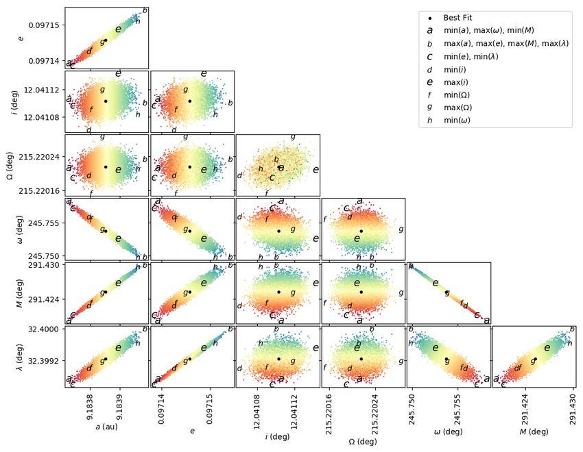
The distribution of orbits generated by this process explicitly shows how the uncertainty of some of
the orbital parameters are strongly coupled, as can be seen in Figure 2. From these 10,000 clones,
we identified the most extreme orbits (largest and smallest value of each parameter) and integrated
these 8 clones (labelled in Figure 2) as well as the best fit orbit. These dynamical integrations
were done using Rebound (Rein & Liu 2012) with the WHFast(Wisdom & Holman 1991; Kinoshita
et al. 1991; Rein & Tamayo 2015) symplectic integrator. The eight major planets and Pluto2 were
included as massive perturbers and an integration step size of 5% of Mercury’s initial orbital period
(' 0.012 yr ' 4.39 days) was used, while output was saved approximately 3 times per year. As
can be seen in Figures 3 and 4, the future evolution of all of the clones involve an initial period in
coorbital resonance, but all clones leave the resonance between 6 kyr and 26 kyr from now. The
large range of resonance exit times is due to the highly chaotic nature of the orbit. We used a
second set of numerical integrations, where clones were displaced infinitesimally (10−13 –10−12 AU, or
1.5–15 cm) relative to each of the above clones, to estimate the object’s current timescale for chaotic
divergence (the Lyapunov time scale); we found this to be 410±60 yr3 . 2013 VZ70 is thus definitely in
coorbital resonance now, but the chaotic nature of the orbit means that the duration of this temporary
resonance capture will likely not be constrained further, even with additional observations.
3. DERIVING THE STEADY STATE ORBITAL DISTRIBUTION
We proceed to investigate the potential origin of temporary coorbitals like 2013 VZ70 . We model the
source of the giant planet temporary coorbitals and investigate their detectability in characterised
surveys. We produced a steady-state distribution of scattering objects in the a < 34 au region
from orbital integrations similar to those used in Alexandersen et al. (2013); the details of those
integrations can be found in the supplementary material of that paper. We primarily outline the
deviations from those used in the previous paper below.
2
Pluto was primarily included as a test to ensure that the system was set up correctly, not because we expect the mass
of Pluto to have any influence on the outcome of the integration. However, since Pluto’s mass is known, there was no
reason to not include it. Pluto was confirmed to be resonating in the 3:2 resonance with Neptune in our integrations,
as expected.
3
A Jupyter notebook demonstrating how the Lyapunov time scale was calculated is available at DOI: 10.11570/21.0008.2013 VZ70 and the Temporary Coorbitals of the Giant Planets 9 Figure 2. Orbital elements of 10,000 fits to resampled astrometry. Each clone was generated using Find_Orb’s MCMC feature, using a Gaussian noise equal to the mean residual of the best fit orbit (0.00 146). The clones are color coded by semi-major axis (which is also the x-axis of the left most row) to give an additional rough indicator of its correlation with the other orbital elements. The best fit orbit is marked with a black dot, and orbits with either the smallest or largest value of one of the parameters are marked with a letter ((a-h, not to be confused with any orbital elements). This figure demonstrates how the uncertainties on the different parameters are related; most parameters are strongly coupled, while i and Ω have only weak or no coupling with other parameters. To perform the dynamical integrations, we used the N-body code SWIFT-RMVS4 (provided by Hal Levison, based on the original SWIFT (Levison & Duncan 1994)) with a base time step of 25 days and an output interval of 50 years for the orbital elements of the planets and any particle which
10                                         Alexandersen et al.

Figure 3.    Future evolution of 2013 VZ70 , the temporary Saturnian horseshoe coorbital. The nine clones
marked on Figure 2 were integrated (the best fit orbit plus eight extremal clones). For clarity, clone trajec-
tories have only been drawn until the semi-major axis of the clone deviates from Saturn’s by more than 1 au
for the first time. The top right panel has been expanded in Figure 4 to better show the clones’ interactions
with the resonance. The "stair step" patterns occurs at the time when φ11 is close to 0◦ /360◦ , which is the
time the coorbital is closest to the planet; the close approach causes the switch from a slightly-larger-than-
the-planet’s semi-major axis to a slightly-smaller-than-the-planet’s (and vice versa) that ensures that the
planet/coorbital never overtake each other. The close approaches also imparts small changes in the other
orbital elements, seen as the "stair step" pattern.

at the moment had a < 34 au. The gravitational influences of the four giant planets and the Sun
were included. The system starts with 8500 particles, derived from the 34 au < a < 200 au scattering
2013 VZ70 and the Temporary Coorbitals of the Giant Planets                                      11

Figure 4.    Future evolution of the resonant angle φ11 (with respect to Saturn) for each of the 2013 VZ70
clones shown in Figures 2 and 3. The information here is identical to that in the top-right subplot of Figure 3,
but split up for clarity. As in Figure 3, clone trajectories have only been drawn until the semi-major axis of
the clone deviates from Saturn’s by more than 1 au for the first time. It is clear that 2013 VZ70 is currently
in the Saturnian coorbital resonance, but will escape from this state in 6–26 kyr. Note that after leaving
the resonance, the minimum Ω clone gets recaptured and librates a few times in each Trojan island before
becoming re-ejected.

portion of the Kaib et al. (2011) model of the outer Solar System. Particles were removed from the
simulation when they hit a planet, went outside 2000 AU or inside 2 AU from the Sun (since they

would either interact with the terrestrial planets that are absent in our simulations or would rapidly
be removed from the Solar System by Jupiter), or the final integration time of 1 Gyr was reached.
Since 1 Gyr is substantially longer than the dynamical lifetime of Centaurs and scattering TNOs,

we thoroughly sample the a
12                                      Alexandersen et al.

100 Myr is similar enough to the distribution in the following 900 Myr (because the a
2013 VZ70 and the Temporary Coorbitals of the Giant Planets                              13

4000 times fewer coorbitals than Neptune), although this is unsurpring given that the source of the
scattering objects is beyond Neptune and that the dynamical timescales (orbital period, libration

timescale) are longer farther from the Sun. An interesting result is that while Neptune’s and Uranus’
coorbitals are roughly equally distributed between horseshoe and Trojan coorbitals, Saturn seems to
very preferentially capture scattering objects into horseshoe orbits, and Jupiter has a much larger

fraction of quasi-satellites than any of the other planets. Table 1 also shows the mean, median and
maximum duration of a capture in coorbital resonance with the planets, as well as the mean, median
and maximum number of captures experienced by particles with at least one episode of coorbital

motion with a given planet. The mean and median coorbital lifetimes and number of captures for
Uranus and Neptune are also within a factor of two of those in Alexandersen et al. (2013), which
we thus adopt as the uncertainty. Note that the captures into coorbital motion with Saturn and

Jupiter are typically significantly shorter than for Uranus and Neptune, although if the lifetimes are
represented in units of orbital periods rather than years, the Jovian captures actually have the second
longest lifetimes, after Uranus. While the different coorbital resonances no doubt experience different

interactions with secular resonances and experience different perturbations from neighbouring planets,
it is noteworthy that the median number of orbital periods for coorbital captures for all four planets
are within a factor of 2.5 of each other. However, going Neptune to Jupiter, particles are increasingly

unlikely to have multiple captures, presumably due to the increasing ability of the planet to scatter
the object to large semi-major axis; this results in particles on average spending both more total
time and more total orbital periods in coorbital motion with Uranus and Neptune than Saturn and

Jupiter.

                        4. COMPARING THEORY AND OBSERVATIONS

 In order to compare our dynamical model to the real detections, we run the model through the
OSSOS Survey Simulator (Bannister et al. 2018; Lawler et al. 2018a). The survey simulator generates
one object at a time (with an orbit drawn from the dynamical model and an H-magnitude drawn from

a parametric model discussed later) and assesses whether the object would have been discovered by
the input surveys. We used all of the characterized surveys with sufficient characterization available
14 Alexandersen et al.
Table 1. Steady state fractions of the a < 34 AU, q > 2 AU scattering objects that are in temporary co-orbital resonance with
the giant planets. For reference, “Horseshoe” coorbitals librate about φ11 = 180◦ , “Trojan” librate about φ11 = 60◦ and 300◦ ,
and “Quasi-satellites” librate about φ11 = 0◦ . Also listed are the mean, median and maximum duration of such captures seen in
our simulations, and the median lifetime divided by the orbital period of the associated planet. Lastly the mean, median and
maximum number of captures experienced by a particle that is trapped by the planet at least once.
Planet Coorbitals Horseshoe Trojan Quasi-satellite Lifetime (kyr) Median lifetime Number of traps
% of scattering % of planet’s coorbitals Mean Median Max (orbital periods) Mean Median Max
Jupiter 0.00093 33 21 46 11 7.1 26 600 1 1 1
Saturn 0.022 85 12 3 19 10 630 340 2 1 6
Uranus 0.65 56 37 7 129 59 16, 000 700 4 2 30
Neptune 3.6 48 40 12 83 46 3, 300 280 10 5 85
for use in the simulator: the Canada-France Ecliptic Plane Survey (CFEPS, Petit et al. 2011), the
CFEPS High-Latitude extension (Petit et al. 2015, HiLat), the Alexandersen et al. (2016) survey,
and OSSOS (Bannister et al. 2018). These surveys combined will be referred to as OSSOS++.
4.1. Orbital distribution
For our survey simulations, it is preferable to have orbital distribution functions rather than an
orbital distribution composed of a fixed number of discrete particles. This allows for the simulator
to be run for as long as necessary, without producing duplicate identical particles. We have set
up independent distributions for the coorbitals and the scattering objects, as described below, both
inspired by the distribution seen in the integrations discussed in Section 3. Our model files and scripts
for use with the OSSOS Survey Simulator (Lawler et al. 2018a) are provided at DOI: 10.11570/21.0008
for anybody curious to use this model distribution.
4.1.1. Scattering objects
We use the output from the Section 3 integrations, taking every particle’s orbit at every time step
and binning them using bin sizes of 0.5 au, 0.02 and 2◦ .0 in a, e and i space. The survey simulator
reads this binned table, randomly selects a bin weighted by the number of particles that went into2013 VZ70 and the Temporary Coorbitals of the Giant Planets 15
the bin, and then randomly assigns a, e and i from a uniform distribution within the bin. Ω, ω
and M are all assigned randomly from a uniform distribution from 0◦ to 360◦ , since the orientations
of scattering objects’ orbits are random. This process allows us to draw essentially infinite unique
particles that follow a distribution consistent with the steady-state distribution from Section 3.
4.1.2. Coorbital objects
We cannot simply bin the coorbital distributions as we did for the scattering distribution. The
numbers of coorbitals in the Section 3 integrations are low (particularly for Jupiter), and the number
of dimensions we would need to bin is higher since the resonant angle φ11 is also important for the
coorbital distribution. Instead, we opted to use parametric distributions, fitted to the distributions
seen in Section 3.
In this simplified parametric model, the semi-major axis of the coorbital is always set equal to that
of the planet, since the few tenths of au variability do not influence detectability by sky surveys as
much as the details of the eccentricity and inclination distribution. The eccentricity is modelled with
a normal distribution, centred at 0 with a width we , multiplied by sin2 (e), truncated to [emin , emax ]4 :
sin2 (e) −e2
f (e|emin ≤ e ≤ emax ) = √ exp (1)
we 2π 2we2
This functional form has little physical motivation and was merely chosen as it in the end provides
a good fit to the distribution seen in our integrations. The inclination is modelled as a normal
distribution, with centre at 0◦ and a width wi , multiplied by sin(i), truncated at imax :
−i2
◦ sin(i)
f (i|0 ≤ i ≤ imax ) = √ exp (2)
wi 2π 2wi2
This is simply a Normal distribution modified to account for the spherical coordinate system. Lastly,
Ω and M are chosen randomly from a uniform distribution [0◦ , 360◦ ) while ω is calculated from φ11 ,
the value of which depends on the type of coorbital. The different types of coorbitals are generated
using the ratios in Table 1. The details of the selection of a φ11 value is similar to that used in
4
In the end, emin ≈ 0.0 was always best, but this was not required.16 Alexandersen et al.
Table 2. Orbital parameters used for each planet
in the parametric model described in Section 4.1.2.
Planet we emin emax wi (◦ ) imax (◦ )
Jupiter 0.188 0.0 0.523 16.1 40.6
Saturn 0.127 0.0 0.707 15.6 89.6
Uranus 0.134 0.0 0.998 19.4 51.3
Neptune 0.123 0.0 0.974 18.1 80.9
Alexandersen et al. (2013), accounting for a distribution of libration amplitudes and the fact that
the centre of libration is offset away from 60◦ /300◦ for Trojans with large libration amplitudes. The
values of we , wi , emin , emax , and imax used in this work for each planet’s coorbital population are
shown in Table 2.
4.2. Absolute magnitude distributions
The Solar System absolute magnitude (H) distribution of the TNOs is not well constrained for
objects fainter than about Hr ≈ 8.0, although it is clear that there is a transition from a steep to
shallower slope somewhere in 7.5 ≤ Hr ≤ 9 (Sheppard & Trujillo 2010; Shankman et al. 2013; Fraser
et al. 2014; Alexandersen et al. 2016; Lawler et al. 2018b). The scattering objects provide a clue to
the small-end distribution, as many of these reach distances closer to the Sun, allowing us to more
easily detect smaller objects. Lawler et al. (2018b) carefully analysed the size distribution of the
scattering objects in OSSOS++; since our sample is a subset of their sample (we only use objects
with a < 34 au), we will directly apply the two magnitude distributions favored by Lawler et al.
(2018b): a divot (with αb = 0.9, αf = 0.5, Hb = 8.3 and c = 3) and a knee (with αb = 0.9, αf = 0.4,
Hb = 7.7 and c = 1). Here αb and αf are the exponent of the exponential magnitude distribution
on the bright and faint (respectively) side of a transition that happens at the break magnitude Hb ; c
denotes the contrast factor of the population immediately on each side of the break, such that c = 1
is a knee and c > 1 is a divot. For further details on this parameterization, see Shankman et al.
(2013) and Lawler et al. (2018b).2013 VZ70 and the Temporary Coorbitals of the Giant Planets 17
4.3. Population estimate
Table 3. Details of the sample (29 objects) used in this work. MPC name denotes the Minor Planet Center
designation for the TNO, while O++ name is the internal designation used within the OSSOS++ surveys.
Cls is the classification of the object, where coorbitals of Saturn, Uranus and Neptune are indicated with
the initial of the planet (S, U, N), with subscripted H, 4 or 5 for horseshoe coorbitals, leading Trojans and
trailing Trojans, respectively; finally C indicates a non-coorbital Centaur/scattering object. Mag is the
magnitude at discovery in the filter F, while H is the absolute magnitude in that same filter. The J2000
barycentric distance, semi-major axis, eccentricity and inclination are shown in d, a, e, i, respectively; for
both d and i the uncertainty is 1 on the last digit or smaller, and has therefore been omitted. The elements
for 2013 VZ70 were calculated using Find_Orb (Gray 2011) and the JPL DE430 planetary ephemerides
(Folkner et al. 2014), while elements for all other objects were taken from Bannister et al. (2018).
MPC O++ Cls Mag F H d a e i
name name (au) (au) ◦
2013 VZ70 Col3N10 SH 23.28 r 13.75 8.891 9.1838 ± 0.0002 0.097145 ± 0.000011 12.041
2015 KJ172 o5m02 C 24.31 r 14.68 9.180 10.8412 ± 0.0018 0.47436 ± 0.00012 11.403
2015 GY53 o5p001 C 24.05 r 13.40 12.029 12.0487 ± 0.0011 0.0828 ± 0.0003 24.112
2015 KH172 o5m01 C 23.55 r 14.92 7.434 16.896 ± 0.004 0.68003 ± 0.00010 9.083
(523790) 2015 HP9 o5p003 C 21.39 r 10.15 13.563 18.146 ± 0.003 0.2699 ± 0.0003 3.070
2011 QF99 mal01 U4 22.57 r 9.56 20.296 19.092 ± 0.003 0.1769 ± 0.0004 10.811
2013 UC17 o3l02 C 23.86 r 11.42 17.045 19.3278 ± 0.0008 0.12702 ± 0.00004 32.476
2015 RE277 o5t01 C 24.02 r 16.13 6.018 20.4545 ± 0.0012 0.766535 ± 0.000014 1.621
2015 RH277 o5s04 C 24.51 r 13.11 13.441 20.916 ± 0.008 0.5083 ± 0.0003 10.109
2015 GB54 o5p004 C 23.92 r 12.68 13.563 20.993 ± 0.007 0.4205 ± 0.0003 1.628
2015 RF277 o5t02 C 24.91 r 14.51 10.616 21.692 ± 0.004 0.51931 ± 0.00013 0.927
2015 RV245 o5s05 C 23.21 r 10.10 19.884 21.981 ± 0.010 0.4793 ± 0.0003 15.389
2013 JC64 o3o01 C 23.39 r 11.95 13.774 22.145 ± 0.002 0.37858 ± 0.00006 32.021
2015 GA54 o5p005 C 24.34 r 10.67 23.500 22.236 ± 0.007 0.2582 ± 0.0006 11.402
2014 UJ225 o4h01 C 22.74 r 10.29 17.756 23.196 ± 0.009 0.3779 ± 0.0004 21.319
2013 UU17 o3l03 C 24.07 r 9.93 25.336 25.87 ± 0.04 0.249 ± 0.003 8.515
2015 RD277 o5t03 C 23.27 r 10.48 18.515 25.9676 ± 0.0014 0.28801 ± 0.00004 18.849
2015 RK277 o5s01 C 23.36 r 15.29 6.237 26.9108 ± 0.0012 0.802736 ± 0.000009 9.533
Table 3 continued on next page18 Alexandersen et al.
Table 3 (continued)
MPC O++ Cls Mag F H d a e i
name name (au) (au) ◦
2014 UG229 o4h02 C 24.33 r 11.47 19.526 27.955 ± 0.005 0.44082 ± 0.00011 12.242
2015 VF164 o5d001 C 23.93 r 12.74 13.286 28.273 ± 0.005 0.54257 ± 0.00013 5.729
2015 VE164 o5c001 C 23.72 r 11.75 15.857 28.529 ± 0.007 0.45711 ± 0.00019 36.539
2012 UW177 mah01 N4 24.20 r 10.61 22.432 30.072 ± 0.003 0.25912 ± 0.00016 53.886
2004 KV18 L4k09 N5 23.64 g 9.33 26.634 30.192 ± 0.003 0.1852 ± 0.0003 13.586
2015 RU245 o5t04 C 22.99 r 9.32 22.722 30.989 ± 0.007 0.2898 ± 0.0003 13.747
2015 GV55 o5p019 C 22.94 r 7.55 34.605 31.375 ± 0.011 0.3026 ± 0.0005 28.287
2008 AU138 HL8a1 C 22.93 r 6.29 44.517 32.393 ± 0.002 0.37440 ± 0.00009 42.826
2015 KS174 o5m04 C 24.38 r 10.19 26.018 32.489 ± 0.005 0.2254 ± 0.0002 7.026
2004 MW8 L4m01 C 23.75 g 8.75 31.360 33.467 ± 0.004 0.33272 ± 0.00008 8.205
2015 VZ167 o5c002 C 23.74 r 11.18 17.958 33.557 ± 0.005 0.52485 ± 0.00009 15.414
We predict a population estimate for the scattering objects with a < 34 au of trans-Neptunian
origin based on our model and the real detections. The OSSOS++ surveys discovered a total of
29 scattering objects with a < 34 au (including 4 temporary coorbitals), listed in Table 3. For the
purposses of this work, 2013 VZ70 is included in this sample, despite its uncharacterized status, as
discussed in subsection 4.5. We thus ran the survey simulation with our scattering model (see Section
4.1.1) as input until it detected 29 objects, recorded how many objects had been drawn from the
model, and repeated 1000 times to measure the uncertainty for the population estimate. For the divot
and knee H distributions respectively, we predict the existence of (2.1±0.2)×107 and (4.9±1.0)×106
scattering TNOs with a < 34 au and Hr < 19. Given the size and orbit distribution, most of these
are small objects beyond 30 au and thus far beyond the detectability both of the surveys we consider
here and similar-depth future surveys like the upcoming Legacy Survey of Space and Time (LSST)
on the Vera Rubin Observatory.
4.4. Expected versus detected numbers
Using the population estimate of the a < 34 au scattering objects as measured in Section 4.3, we
predict the number of temporary coorbitals of TNO origin that OSSOS++ should have detected.2013 VZ70 and the Temporary Coorbitals of the Giant Planets 19 This is done by running the survey simulator for each planet’s coorbital population separately (using the coorbital model defined in Section 4.1.2), inputting a fixed number of coorbital particles (equal to the total scattering object population estimate found in Section 4.3 multiplied by the coorbital fraction for the given planet as found in Section 3) and recording the number of detections, repeating 1000 times to sample the distribution. We find that for both the divot and knee distribution and for each planet, the most common (expected) value of temporary coorbital detections is zero. However, the probabilities of getting zero detected temporary coorbitals for Saturn, Uranus and Neptune are 84%, 74% and 71% (divot) or 91%, 73% and 59% (knee). The probability of getting zero detections for all three planets in these surveys is thus less than 50%. In other words, more often than not, we would expect OSSOS++ to detect at least one giant planet coorbital beyond Jupiter (the case of Jupiter is discussed in the next paragraph). From the distribution of simulated detections, we find that the detection of four coorbitals (as in the real surveys) is unlikely, at a probability of 0.8%, but not completely implausible. We expand on this below. For Jupiter, the chance of zero detections is > 99.99% due to the rate of motion cuts imposed on/by the moving object detection algorithms of the OSSOS++ surveys; only the most eccentric Jovian coorbitals would have been detectable at aphelion (and only in a few fields). It is thus entirely reasonable that OSSOS++ found no Jovian coorbitals, neither temporary nor long term stable; these surveys were simply not sensitive to objects at those distances. We note that there is one known temporary retrograde (i > 90◦ ) coorbital of Jupiter, 2015 BZ509 (514107) Ka‘epaoka‘awela (Wiegert et al. 2017), whose origin is, according to Greenstreet et al. (2020), most likely the main asteroid belt and not the trans-neptunian/scattering object population. Our simulations produce no retrograde coorbitals of any of the planets, supporting that Ka‘epaoka‘awela likely originates from the asteroid belt and not the transneptunian region. Our survey simulations predict a number ratio of detected Jovian, Saturnian, Uranian and Nep- tunian coorbitals of 0:1:2:2 (J:S:U:N, where the mean number of detections have been scaled such that the value for Saturn is 1, then rounded). The ratio of real detections is 0:1:1:2 (2013 VZ70 , 2011 QF99 , 2012 UW177 and 2004 KV18 ), so the ratio of detected temporary coorbitals of each of the giant
20                                     Alexandersen et al.

planets is in good agreement with predictions. However, the survey simulations predict that only 3%
of the detected a < 34 au scattering objects should be coorbitals, whereas the four real coorbitals

make up 14% of detections (4 of 29); the observed fraction of the a < 34 au scattering objects that
are in temporary coorbital resonance is thus ∼ 5 times higher than expected. Before the OSSOS
survey, which was by far the most sensitive survey of the ensemble and discovered over 80% of the

OSSOS++ TNOs and scattering objects, 60% were coorbital (3 of 5), so it would appear that the
initially high fraction of coorbitals detected in the earlier surveys in our set was a fluke, and that
the ratio is approaching the theoretical value predicted above as the observed sample increases. We

thus do not feel it justified to hypothesize additional sources for the temporary coorbital population
at this time. While we cannot rule out that the population of temporary coorbitals, particularly for
Jupiter, is supplemented from other sources such as the asteroid belt and primordial Jovian Trojans,

Greenstreet et al. (2020) finds that for Jovian temporary coorbitals, the asteroid belt is only the
dominant source for retrograde (i > 90◦ ) coorbitals, which they estimate comprise  1% of the tem-
porary coorbital population. It is unlikely that the asteroid belt is a dominant source for the outer

planets if it isn’t for Jupiter. The contribution of the asteroid belt to the steady state temporary
coorbital distribution of the giant planets is thus insignificant, and we are likely not missing any
important source population in producing our population/detection estimates.

                                            4.5. Caveat

 While the orbit of 2013 VZ70 was well determined by the OSSOS observations, it is not part of
the characterized OSSOS dataset. 2013 VZ70 was discovered in images taken in a “failed” observing

sequence from 2013B (failed due to poor image quality and the sequence not being completed),
which was thus not used for the characterised (ie. well understood) part of the OSSOS survey. This
failed sequence, which should have been 30 high-quality images of 10 fields (half of the OSSOS “H”

block), only obtained low-quality (limiting mr ≈ 23.5) images of 6 fields. A TNO search of these
images was conducted (discovering 2013 VZ70 ) to facilitate follow-up observations (color and light
curve measurements), but this shallow search was never characterised due to the expectation that

everything would be rediscovered in an eventual high-quality discovery sequence. A high-quality
2013 VZ70 and the Temporary Coorbitals of the Giant Planets 21
observing sequence of the full set of H-block fields was successfully observed in 2014B, with limiting
magnitude mr = 24.67, which was used for the characterised search. However, as a year had passed,
2013 VZ70 had already left the field due to its large rate of motion; unlike all other objects discovered
in the failed 2013B sequence, 2013 VZ70 was thus not re-discovered in the characterised discovery
images. As such, 2013 VZ70 is not part of the characterised sample of the survey, as that sample
only includes objects discovered in specific images on specific nights through a carefully characterised
process. However, because the failed discovery sequence points at the same area of the sky as parts
of the characterised survey and it is a small minority of the total observed fields, it would make
hardly any difference on the discovery biases whether these particular images are included in the
characterization or not. From our simulations in Section 4 we can see that only about 8% of simulated
detections of theoretical Saturnian Coorbitals were discovered in the OSSOS H block; this block is
thus not in a crucial location for discovering Saturnian coorbitals in any way. The fact that the only
Saturnian coorbital to have been discovered in OSSOS++ was among the very small minority of those
surveys’ total discoveries that were not characterised thus appears to be a low-probability event. We
can therefore treat 2013 VZ70 as effectively being part of the characterised survey for the purposes
of this work, with the warning that this approach should not be used for other non-characterised
objects from these surveys; most other objects are non-characterised for other reasons, mostly for
being fainter than the well-measured part of the detection efficiency function. That being said,
ignoring 2013 VZ70 from the sample on grounds of being uncharacterized would brings the coorbital
to total scattering ratio down to 11% (3 out of 28), closer to the 3% predicted in the previous section.
5. CONCLUSIONS
2013 VZ70 is the first known temporary Saturnian horseshoe coorbital, remaining resonant for 6–
26 kyr; it likely originates in the trans-Neptunian region. Our simulations show that all the giant
planets should have temporary coorbitals of TNO origin, although Jupiter has approximately a factor
of 4000 fewer than Neptune; the duration of the coorbital captures are significantly more short-lived
for Saturn and Jupiter than for Uranus and Neptune. Our simulations show that Neptune’s and
Uranus’ coorbitals should be roughly equally distributed between horseshoe and Trojan coorbitals,22 Alexandersen et al.
Saturn very preferentially captures scattering objects into horseshoe orbits, and Jupiter should have
a much larger fraction of its temporary coorbitals be quasi-satellites than any of the other planets.
Accounting for observing biases in a set of well-characterized surveys (CFEPS (Petit et al. 2011),
HiLat (Petit et al. 2015), the Alexandersen et al. (2016) survey, and OSSOS (Bannister et al. 2018))
we find that the fraction of a < 34 au scattering objects that are in temporary coorbital motion
is higher in the real observations (13.7%) than in simulated observations (2.9%). However, for the
distribution of the temporary coorbitals among the giant planets, we find that our predictions (∼
0:1:2:2 for J:S:U:N) are consistent with the observations (0:1:1:2).
ACKNOWLEDGMENTS
This work is based on TNO discoveries obtained with MegaPrime/MegaCam, a joint project of the
Canada France Hawaii Telescope (CFHT) and CEA/DAPNIA, at CFHT which is operated by the
National Research Council (NRC) of Canada, the Institute National des Sciences de l’Universe of
the Centre National de la Recherche Scientifique (CNRS) of France, and the University of Hawaii. A
portion of the access to the CFHT was made possible by the Academia Sinica Institute of Astronomy
and Astrophysics, Taiwan. This research used the facilities of the Canadian Astronomy Data Centre
operated by the National Research Council of Canada with the support of the Canadian Space
Agency.
The authors wish to recognize and acknowledge the very significant cultural role and reverence that
the summit of Maunakea has always had within the indigenous Hawaiian community. We are most
fortunate to have the opportunity to conduct observations from this mountain. We would also like to
acknowledge the maintenance, cleaning, administrative and support staff at academic and telescope
facilities, whose labor maintains the spaces where astrophysical inquiry can flourish.
The authors wish to thank Hanno Rein for useful discussions and help regarding how to estimate
the Lyapunov timescale through numerical integrations. The authors also wish to thank Jeremy
Wood for the suggestion of looking at the capture durations in terms of orbital periods rather than
only absolute time.2013 VZ70 and the Temporary Coorbitals of the Giant Planets 23 SG acknowledges support from the Asteroid Institute, a program of B612, 20 Sunnyside Ave, Suite 427, Mill Valley, CA 94941. Major funding for the Asteroid Institute was generously provided by the W.K. Bowes Jr. Foundation and Steve Jurvetson. Research support is also provided from Founding and Asteroid Circle members K. Algeri-Wong, B. Anders, R. Armstrong, G. Baehr, The Barringer Crater Company, B. Burton, D. Carlson, S. Cerf, V. Cerf, Y. Chapman, J. Chervenak, D. Corrigan, E. Corrigan, A. Denton, E. Dyson, A. Eustace, S. Galitsky, L. & A. Fritz, E. Gillum, L. Girand, Glaser Progress Foundation, D. Glasgow, A. Gleckler, J. Grimm, S. Grimm, G. Gruener, V. K. Hsu & Sons Foundation Ltd., J. Huang, J. D. Jameson, J. Jameson, M. Jonsson Family Foundation, D. Kaiser, K. Kelley, S. Krausz, V. Lašas, J. Leszczenski, D. Liddle, S. Mak, G.McAdoo, S. McGregor, J. Mercer, M. Mullenweg, D. Murphy, P. Norvig, S. Pishevar, R. Quindlen, N. Ramsey, P. Rawls Family Fund, R. Rothrock, E. Sahakian, R. Schweickart, A. Slater, Tito’s Handmade Vodka, T. Trueman, F. B. Vaughn, R. C. Vaughn, B. Wheeler, Y. Wong, M. Wyndowe, and nine anonymous donors. SG acknowledges the support from the University of Washington College of Arts and Sciences, Department of Astronomy, and the DIRAC Institute. The DIRAC Institute is supported through generous gifts from the Charles and Lisa Simonyi Fund for Arts and Sciences and the Washington Research Foundation. This work was supported in part by NASA NEOO grant NNX14AM98G to LCOGT/Las Cumbres Observatory. KV acknowledges support from NASA (grants NNX15AH59G and 80NSSC19K0785) and NSF (grant AST-1824869). This work was supported by the Programme National de Plantologie (PNP) of CNRS-INSU co- funded by CNES. This research has made use of NASA’s Astrophysics Data System Bibliographic Services. This research made use of SciPy (Jones et al. 2001), NumPy (van der Walt et al. 2011), matplotlib (a Python library for publication quality graphics, Hunter 2007). Facilities: CFHT(MegaCam)
24                                         Alexandersen et al.

 Software: Python (van Rossum & de Boer 1991), Matplotlib (Hunter 2007), NumPy (van der
Walt et al. 2011), SciPy (Jones et al. 2001), Find_Orb (Gray 2011), Rebound (Rein & Liu 2012),

fit_radec & abg_to_aei (Bernstein & Khushalani 2000), SWIFT-RMVS4 (Levison & Duncan 1994),
Jupyter notebook (Kluyver et al. 2016)

                                              REFERENCES

Alexandersen, M., Gladman, B., Greenstreet, S.,       Boulade, O., Charlot, X., Abbon, P., et al. 2003,
  et al. 2013, Science, 341, 994,                       Instrument Design and Performance for
  doi: 10.1126/science.1238072                          Optical/Infrared Ground-based Telescopes.
                                                        Edited by Iye, 4841, 72
Alexandersen, M., Gladman, B., Kavelaars, J. J.,
  et al. 2016, AJ, 152, 111,                          Bowell, E., Holt, H. E., Levy, D. H., et al. 1990, in

  doi: 10.3847/0004-6256/152/5/111                      BAAS, Vol. 22, 1357

                                                      Ćuk, M., Hamilton, D. P., & Holman, M. J. 2012,
Alvarez-Candal, A., & Roig, F. 2005, in IAU
                                                        MNRAS, 426, 3051,
  Colloq. 197: Dynamics of Populations of
                                                        doi: 10.1111/j.1365-2966.2012.21964.x
  Planetary Systems, ed. Z. Knežević & A. Milani,
  205–208, doi: 10.1017/S174392130400866X             de la Barre, C. M., Kaula, W. M., & Varadi, F.
                                                        1996, Icarus, 121, 88,
Bannister, M. T., Kavelaars, J., Gladman, B. J.,
                                                        doi: 10.1006/icar.1996.0073
  et al. 2021, Minor Planet Electronic Circulars,
  2021-Q55                                            Duncan, M. J., & Levison, H. F. 1997, Science,
                                                        276, 1670, doi: 10.1126/science.276.5319.1670
Bannister, M. T., Kavelaars, J. J., Petit, J.-M.,
                                                      Dvorak, R., Bazsó, Á., & Zhou, L.-Y. 2010,
  et al. 2016, AJ, 152, 70,
                                                        Celestial Mechanics and Dynamical Astronomy,
  doi: 10.3847/0004-6256/152/3/70
                                                        107, 51, doi: 10.1007/s10569-010-9261-y
Bannister, M. T., Gladman, B. J., Kavelaars, J. J.,
                                                      Folkner, W. M., Williams, J. G., Boggs, D. H.,
  et al. 2018, The Astrophysical Journal
                                                        Park, R. S., & Kuchynka, P. 2014,
  Supplement Series, 236, 18,
                                                        Interplanetary Network Progress Report,
  doi: 10.3847/1538-4365/aab77a
                                                        42-196, 1

Bernstein, G., & Khushalani, B. 2000, AJ, 120,        Fountain, J. W., & Larson, S. M. 1978, Icarus, 36,
  3323, doi: 10.1086/316868                             92, doi: 10.1016/0019-1035(78)90076-3
2013 VZ70 and the Temporary Coorbitals of the Giant Planets 25
Fraser, W. C., Brown, M. E., Morbidelli, A., Kaib, N. A., Roškar, R., & Quinn, T. 2011, Icarus,
Parker, A., & Batygin, K. 2014, ApJ, 782, 100, 215, 491, doi: 10.1016/j.icarus.2011.07.037
doi: 10.1088/0004-637X/782/2/100 Karlsson, O. 2004, Astronomy and Astrophysics,
Gomes, R., & Nesvorný, D. 2016, A&A, 592, 413, 1153, doi: 10.1051/0004-6361:20031543
A146, doi: 10.1051/0004-6361/201527757
Kinoshita, H., Yoshida, H., & Nakai, H. 1991,
Gray, B. 2011, Find_Orb: Orbit determination
Celestial Mechanics and Dynamical Astronomy,
from observations.
50, 59
https://www.projectpluto.com/find_orb.htm
Kluyver, T., Ragan-Kelley, B., Pérez, F., et al.
Greenstreet, S., Gladman, B., & Ngo, H. 2020, AJ,
2016, in Positioning and Power in Academic
160, 144, doi: 10.3847/1538-3881/aba2c9
Publishing: Players, Agents and Agendas, ed.
Holman, M. J., & Wisdom, J. 1993, AJ, 105, 1987,
F. Loizides & B. Schmidt, IOS Press, 87 – 90
doi: 10.1086/116574
Lawler, S. M., Kavelaars, J. J., Alexandersen, M.,
Horner, J., & Lykawka, P. S. 2012, Monthly
et al. 2018a, Frontiers in Astronomy and Space
Notices of the Royal Astronomical Society, 426,
Sciences, 5, 14, doi: 10.3389/fspas.2018.00014
159, doi: 10.1111/j.1365-2966.2012.21717.x
Horner, J., & Wyn Evans, N. 2006, Monthly Lawler, S. M., Shankman, C., Kavelaars, J. J.,
Notices of the Royal Astronomical Society, 367, et al. 2018b, AJ, 155, 197,
L20, doi: 10.1111/j.1745-3933.2006.00131.x doi: 10.3847/1538-3881/aab8ff
Hou, X. Y., Scheeres, D. J., & Liu, L. 2014, Levison, H. F., & Duncan, M. J. 1994, Icarus, 108,
MNRAS, 437, 1420, doi: 10.1093/mnras/stt1974 18, doi: 10.1006/icar.1994.1039
Huang, Y., Li, M., Li, J., & Gong, S. 2019, Levison, H. F., Shoemaker, E. M., & Shoemaker,
MNRAS, 488, 2543, doi: 10.1093/mnras/stz1840 C. S. 1997, Nature, 385, 42,
Hunter, J. D. 2007, Computing In Science & doi: 10.1038/385042a0
Engineering, 9, 90
Li, M., Huang, Y., & Gong, S. 2018, A&A, 617,
Innanen, K. A., & Mikkola, S. 1989, AJ, 97, 900,
A114, doi: 10.1051/0004-6361/201833019
doi: 10.1086/115036
Lykawka, P. S., & Mukai, T. 2007, Icarus, 192,
Jedicke, R., Bolin, B. T., Bottke, W. F., et al.
238, doi: 10.1016/j.icarus.2007.06.007
2018, Frontiers in Astronomy and Space
Marzari, F., & Scholl, H. 2000, Icarus, 146, 232,
Sciences, 5, 13, doi: 10.3389/fspas.2018.00013
doi: 10.1006/icar.2000.6376
Jones, E., Oliphant, T., Peterson, P., & Others.
2001, SciPy: Open source scientific tools for Marzari, F., Tricarico, P., & Scholl, H. 2003, A&A,
Python. http://www.scipy.org/ 410, 725, doi: 10.1051/0004-6361:2003127526 Alexandersen et al. Mikkola, S., Brasser, R., Wiegert, P., & Innanen, Scholl, H., Marzari, F., & Tricarico, P. 2005, K. 2004, Monthly Notices of the Royal Icarus, 175, 397, Astronomical Society, 351, L63, doi: 10.1016/j.icarus.2005.01.018 doi: 10.1111/j.1365-2966.2004.07994.x Shankman, C., Gladman, B. J., Kaib, N., Mikkola, S., Innanen, K., Wiegert, P., Connors, Kavelaars, J. J., & Petit, J. M. 2013, M., & Brasser, R. 2006, MNRAS, 369, 15, Astrophysical Journal Letters, 764, L2, doi: 10.1111/j.1365-2966.2006.10306.x doi: 10.1088/2041-8205/764/1/L2 Morbidelli, A., Levison, H. F., Tsiganis, K., & Sheppard, S. S., & Trujillo, C. A. 2010, Gomes, R. 2005, Nature, 435, 462, Astrophysical Journal Letters, 723, L233, doi: 10.1038/nature03540 doi: 10.1088/2041-8205/723/2/L233 Murray, C. D., & Dermott, S. F. 1999, Solar Tsiganis, K., Varvoglis, H., & Hadjidemetriou, system dynamics (Cambridge University Press), J. D. 2000, Icarus, 146, 240, 63–129 doi: 10.1006/icar.2000.6382 Nesvorný, D., & Dones, L. 2002, Icarus, 160, 271, van der Walt, S., Colbert, S. C., & Varoquaux, G. doi: 10.1006/icar.2002.6961 2011, Computing in Science Engineering, 13, 22, Nesvorný, D., Vokrouhlický, D., & Morbidelli, A. doi: 10.1109/MCSE.2011.37 2013, ApJ, 768, 45, van Rossum, G., & de Boer, J. 1991, in EurOpen. doi: 10.1088/0004-637X/768/1/45 UNIX Distributed Open Systems in Perspective. Parker, A. H. 2015, Icarus, 247, 112, Proceedings of the Spring 1991 EurOpen doi: 10.1016/j.icarus.2014.09.043 Conference, Tromsø, Norway, May 20–24, 1991, Petit, J.-M., Kavelaars, J. J., & Gladman, B. J. ed. EurOpen (Buntingford, Herts, UK: 2015, In prep EurOpen), 229–247 Petit, J.-M., Kavelaars, J. J., Gladman, B. J., Volk, K., Murray-Clay, R. A., Gladman, B. J., et al. 2011, Astronomical Journal, 142, 131, et al. 2018, AJ, 155, 260, doi: 10.1088/0004-6256/142/4/131 doi: 10.3847/1538-3881/aac268 Polishook, D., Jacobson, S. A., Morbidelli, A., & Wiegert, P., Connors, M., & Veillet, C. 2017, Aharonson, O. 2017, Nature Astronomy, 1, Nature, 543, 687, doi: 10.1038/nature22029 0179, doi: 10.1038/s41550-017-0179 Wiegert, P. A., Innanen, K. A., & Mikkola, S. Rein, H., & Liu, S. F. 2012, A&A, 537, A128, 1998, Astronomical Journal, 115, 2604, doi: 10.1051/0004-6361/201118085 doi: 10.1086/300358 Rein, H., & Tamayo, D. 2015, MNRAS, 452, 376, Wisdom, J., & Holman, M. 1991, AJ, 102, 1528, doi: 10.1093/mnras/stv1257 doi: 10.1086/115978
2013 VZ70 and the Temporary Coorbitals of the Giant Planets   27

Wolf, M. 1906, Astronomische Nachrichten, 170,
  353
Yu, T. Y. M., Murray-Clay, R., & Volk, K. 2018,
  AJ, 156, 33, doi: 10.3847/1538-3881/aac6cd
You can also read