Partition Function Estimation: A Quantitative Study - IJCAI
←
→
Page content transcription
If your browser does not render page correctly, please read the page content below
Proceedings of the Thirtieth International Joint Conference on Artificial Intelligence (IJCAI-21)
                                                                   Survey Track

                       Partition Function Estimation: A Quantitative Study

                            Durgesh Agrawal1 , Yash Pote2 and Kuldeep S. Meel2
                             1
                               Indian Institute of Technology Kanpur, Kanpur, India
                                  2
                                    National University of Singapore, Singapore

                         Abstract                                             work of Roth (1996) established that the problem of com-
                                                                              putation of partition function is #P-hard. Since the parti-
     Probabilistic graphical models have emerged as a                         tion function plays a crucial role in probabilistic reasoning,
     powerful modeling tool for several real-world sce-                       the development of algorithmic techniques for calculating
     narios where one needs to reason under uncertainty.                      the partition function has witnessed a sustained interest from
     A graphical model’s partition function is a central                      practitioners over the years [McCallum et al., 2009; Molka-
     quantity of interest, and its computation is key to                      raie and Loeliger, 2012; Gillespie, 2013; Ma et al., 2013;
     several probabilistic reasoning tasks. Given the #P-                     Waldorp and Marsman, 2019].
     hardness of computing the partition function, sev-                          The algorithms can be broadly classified into three cate-
     eral techniques have been proposed over the years                        gories based on the quality of computed estimates:
     with varying guarantees on the quality of estimates
                                                                                1. Exact [Pearl, 1986; Lauritzen and Spiegelhalter, 1988;
     and their runtime behavior. This paper seeks to
                                                                                    Pearl, 1988; Horvitz et al., 1989; Jensen et al., 1990;
     present a survey of 18 techniques and a rigorous
                                                                                    Mateescu and Dechter, 1990; Darwiche, 1995; Dechter,
     empirical study of their behavior across an exten-
                                                                                    1996; Dechter, 1999; Darwiche, 2001b; Chavira et al.,
     sive set of benchmarks. Our empirical study draws
                                                                                    2004; Darwiche, 2004; Mateescu and Dechter, 2005;
     up a surprising observation: exact techniques are as
                                                                                    Darwiche, 2011; Lagniez and Marquis, 2017]
     efficient as the approximate ones, and therefore, we
     conclude with an optimistic view of opportunities                          2. Approximate [Jerrum and Sinclair, 1993; Darwiche,
     for the design of approximate techniques with en-                              1995; Gogate and Dechter, 2005; Georgiev et al., 2012;
     hanced scalability. Motivated by the observation of                            Ermon et al., 2013a; Ermon et al., 2013b; Kuck et al.,
     an order of magnitude difference between the Vir-                              2018; Lee et al., 2019; Kuck et al., 2019; Sharma et al.,
     tual Best Solver and the best performing tool, we                              2019]
     envision an exciting line of research focused on the                       3. Guarantee-less [Pearl, 1982; Yedidia et al., 2000;
     development of portfolio solvers.                                              Minka, 2001; Dechter et al., 2002; Wiegerinck and Hes-
                                                                                    kes, 2003; Qi and Minka, 2004; Eaton and Ghahramani,
                                                                                    2009; Liu and Ihler, 2011; Kuck et al., 2020]
1   Introduction                                                              While the exact techniques return an accurate result, the ap-
Probabilistic graphical models are ubiquitously employed to                   proximate methods typically provide (ε, δ) guarantees such
capture probabilistic distributions over complex structures                   that the returned estimate is within ε factor of the true value
and therefore find applications in a wide variety of do-                      with confidence of at least 1 − δ. Finally, the guarantee-less
mains [Darwiche, 2009; Koller and Friedman, 2009; Mur-                        methods return estimates without any accuracy or confidence
phy, 2012]. For instance, image segmentation and recogni-                     guarantees. Another classification of the algorithmic tech-
tion can be modeled into a statistical inference problem [Fan                 niques can be achieved based on the usage of underlying core
and Fan, 2008]. In computational protein design, by model-                    technical ideas:
ing force fields of a protein and another target molecule as                    1. Message passing [Pearl, 1982; Yedidia et al., 2000;
Markov Random Fields and computing partition function for                           Minka, 2001; Wainwright et al., 2001; Dechter et al.,
the molecules in bound and unbound states, their affinity can                       2002; Wiegerinck and Heskes, 2003; Qi and Minka,
be estimated [Viricel et al., 2016].                                                2004; Eaton and Ghahramani, 2009]
   Given a probabilistic graphical model where the nodes cor-
respond to variables of interest, one of the fundamental prob-                  2. Variable elimination [Dechter, 1996; Dechter, 1999; Liu
lems is computing the normalization constant or the partition                       and Ihler, 2011; Peyrard et al., 2019; Lee et al., 2019]
function. Calculation of the partition function is computa-                     3. Model counting [Darwiche, 2001a; Chavira et al., 2004;
tionally intractable owing to the need for summation over                           Chavira and Darwiche, 2007; Darwiche, 2011; Ermon
possibly exponentially many terms. Formally, the seminal                            et al., 2013a; Ermon et al., 2013b; Viricel et al., 2016;

                                                                       4276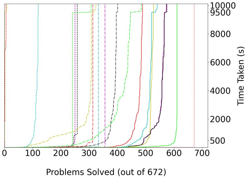
Proceedings of the Thirtieth International Joint Conference on Artificial Intelligence (IJCAI-21)
                                                                      Survey Track

       Lagniez and Marquis, 2017; Grover et al., 2018; Shu                       Xu et al., 2008] and we envision development of such solvers
       et al., 2018; Sharma et al., 2019; de Colnet and Meel,                    in the context of partition function.
       2019; Wu et al., 2019; Lagniez and Marquis, 2019; Shu                        The remainder of this paper is organized as follows. In Sec-
       et al., 2019; Wu et al., 2020; Agrawal et al., 2020; Meel                 tion 2, we introduce the preliminaries while Section 3 surveys
       and Akshay, 2020; Soos et al., 2020; Zeng et al., 2020;                   different techniques for partition function estimation. In Sec-
       Dudek et al., 2020]                                                       tion 4, we describe the objectives of our experimental evalu-
 4. Sampling [Henrion, 1988; Shachter and Peot, 1989;                            ations, the setup, and the benchmarks used. We present our
    Doucet et al., 2000; Winkler, 2002; Gogate and Dechter,                      experimental findings in Section 5. The paper is concluded in
    2005; Ermon et al., 2011; Gogate and Dechter, 2011;                          Section 6.
    Ma et al., 2013; Liu et al., 2015; Lou et al., 2017;
    Broka et al., 2018; Saeedi et al., 2017; Cundy and Er-                       2     Preliminaries
    mon, 2020; Pabbaraju et al., 2020].
                                                                                 A graphical model consists of variables and factors. We rep-
   Given the plethora of techniques, their relative perfor-                      resent sets in bold, and their elements in regular typeface.
mance may not always be apparent to a practitioner. It may
                                                                                    Let X = {x1 , x2 , ..., xn } be the set of discrete random vari-
contribute to the non-usage of the state-of-the-art method,
                                                                                 ables. Let us consider a family S ⊆ 2X . For each x ∈ S, we
thereby limiting the potential offered by probabilistic graphi-
                                                                                 use fx to denote a factor, which is a function defined over x.
cal models. In particular, we draw inspiration from a related
                                                                                 fx returns a non-negative real value for each assignment σ(x)
sub-field of automated reasoning: SAT solving, where a de-
                                                                                 where each variable in x is assigned a value from its domain.
tailed evaluation of SAT solvers offered by SAT competition
                                                                                 In other words, if Dx denotes the cross product of domains
informs the practitioners of the state-of-the-art [Heule et al.,
                                                                                 of all variables in x, then fx : Dx → R+
2019]. An essential step in this direction was taken by the or-
ganization of the six UAI Inference challenges from 2008 to                         The probability distribution is often represented as a bi-
2016 1 . While these challenges have highlighted the strengths                   partite graph, called a factor graph G = (X ∪ S, E), where
and weaknesses of the different techniques, a large selection                    (xi , x) ∈ E iff xi ∈ x.
of algorithmic techniques has not been evaluated owing to a                         The probability distribution encoded by the factor graph is
lack of submissions of the corresponding tools to these com-                                    1 Q
                                                                                 P (σ(X)) =            fx (σ(x)), where the normalization con-
petitions.                                                                                      Z x∈S
   This survey paper presents a rigorous empirical study span-                   stant, denoted by Z and also called partition function, is de-
ning 18 techniques proposed by the broader UAI commu-                            fined as
nity over an extensive set of benchmarks. To the best of our                                                 X Y
knowledge, this is the most comprehensive empirical study to                                         Z :=             fx (σ(x))
understand the behavior of different techniques for computa-                                                    σ(X) x∈S
tion of partition function/normalization constant. Given that
computation of the partition function is a functional problem,                       We focus on techniques for the computation of Z.
we design a new metric to enable runtime comparison of dif-
ferent techniques for problems where the ground truth is un-                     3     Overview of Algorithms
known. To judge long-running or non-terminating algorithms
fairly, we use a two-step timeout that allows them to provide                    We provide an overview of the central ideas behind the algo-
sub-optimal answers. Our proposed metric, TAP score, cap-                        rithms we have included in this study. The algorithms can be
tures both the time taken by a method and its computation ac-                    broadly classified into four categories based on their funda-
curacy relative to other techniques on a unified numeric scale.                  mental approach:
   Our empirical study throws up several surprising observa-
tions: the weighted counting-based technique, Ace [Chavira                       3.1    Message Passing-based Techniques
and Darwiche, 2005] solves the largest number of prob-
lems closely followed by loopy and fractional belief prop-                       Message Passing algorithms involve sending messages be-
agation. While Ace falls in the category of exact meth-                          tween objects that could be variable nodes, factor nodes, or
ods, several of the approximate and guarantee-less tech-                         clusters of variables, depending on the algorithm. Eventu-
niques, surprisingly, perform poorly compared to the exact                       ally, some or all the objects inspect the incoming messages
techniques. Given the #P-hardness of computing the parti-                        to compute a belief about what their state should be. These
tion function, the relatively weak performance of approxi-                       beliefs are used to calculate the value of Z.
mate techniques should be viewed as an opportunity for fu-                       Loopy Belief Propagation was first proposed by Pearl
ture research. Furthermore, we observe that for every prob-                      (1982) for exact inference on tree-structured graphical mod-
lem, at least one method was able to solve in less than 20                       els [Kschischang et al., 2001]. The sum-product variant of
seconds with a 32-factor accuracy. Such an observation                           LBP is used for computing the partition function. For general
in the context of SAT solving led to an exciting series of                       models, the algorithm’s convergence is not guaranteed, and
works on the design of portfolio solvers [Hutter et al., 2007;                   the beliefs computed upon convergence may differ from the
                                                                                 true marginals. The point of convergence corresponds to a
   1
       www.hlt.utdallas.edu/∼vgogate/uai16-evaluation                            local minimum of Bethe free energy.

                                                                          4277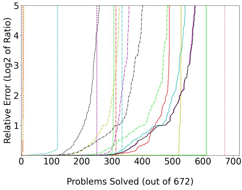
Proceedings of the Thirtieth International Joint Conference on Artificial Intelligence (IJCAI-21)
                                                                    Survey Track

Conditioned Belief Propagation Conditioned Belief Prop-                        a variable ordering, the bucket associated with a variable x
agation is a modification of LBP. Initially, Conditioned BP                    does not contain factors that are a function of variables higher
chooses a variable x and a state X and performs Back Belief                    than x in the ordering. Subsequently, the buckets are pro-
Propagation (back-propagation applied to Loopy BP) with x                      cessed from last to first. When the bucket of variable x is pro-
clamped to X (i.e., conditioned on x = X), and also with                       cessed, an elimination procedure is performed over its func-
the negation of this condition. The process is done recur-                     tions, yielding a new function f that does not mention x, and
sively up to a fixed number of levels. The resulting approxi-                  f is placed in a lower bucket. The algorithm performs exact
mate marginals are combined using estimates of the partition                   inference, and the time and space complexity are exponential
sum [Eaton and Ghahramani, 2009].                                              in the problem’s induced width [Dechter, 1996].
Fractional Belief Propagation modifies LBP by associating                      Weighted Mini Bucket Elimination is a generalization of
each factor with a weight. If each factor f has weight wf ,                    Mini-Bucket Elimination, which is a modification of Bucket
then the algorithms minimize the α-divergence [Amari et al.,                   Elimination and performs approximate inference. It partitions
2001] with α = 1/wf for that factor [Wiegerinck and Heskes,                    the factors in a bucket into several mini-buckets such that at
2003]. Setting all the weights to 1 reduces FBP to Loopy                       most iBound variables are allowed in a mini-bucket. The
Belief Propagation.                                                            accuracy and complexity increase as iBound increases.
Generalized Belief Propagation modifies LBP so that mes-                          Weighted Mini Bucket Elimination associates a weight
sages are passed from a group of nodes to another group of                     with each mini-bucket and achieves a tighter upper bound on
nodes [Yedidia et al., 2000]. Intuitively, the messages trans-                 the partition function based on Holder’s inequality [Liu and
ferred by this approach are more informative, thus improving                   Ihler, 2011].
inference. The convergence points of GBP are equivalent to
the minima of the Kikuchi free energy.                                         3.3    Model Counting-based Techniques
Edge Deletion Belief Propagation is an anytime algorithm
                                                                               Partition function computation can be reduced to one of the
that starts with a tree-structured approximation correspond-
                                                                               weighted model counting [Darwiche, 2002]. A factor graph
ing to loopy BP, and incrementally improves it by recovering
                                                                               is first encoded into a CNF formula ϕ, with an associated
deleted edges [Choi and Darwiche, 2006].
                                                                               weight function W assigning weights to literals such that the
HAK Algorithm Whenever Generalised BP [Yedidia et al.,
                                                                               weight of an assignment is the product of the weight of its
2000] reaches a fixed point, it is known that the fixed point
                                                                               literals. Given ϕ and W , computing the partition function re-
corresponds to the extrema of the Kikuchi free energy. How-
                                                                               duces to computing the sum of weights of satisfying assign-
ever, generalized BP does not always converge. The HAK
                                                                               ments of ϕ, also known as weighted model counting [Chavira
algorithm solves this typically non-convex constrained mini-
                                                                               and Darwiche, 2008].
mization problem through a sequence of convex constrained
                                                                               Weighted Integral by Sums and Hashing(WISH) reduces
minimizations of upper bounds on the Kikuchi free en-
                                                                               the problem into a small number of optimization queries sub-
ergy [Heskes et al., 2003].
                                                                               ject to parity constraints used as hash functions. It computes a
Join Tree partitions the graph into clusters of variables such
                                                                               constant-factor approximation of partition function with high
that the interactions among clusters possess a tree structure,
                                                                               probability [Ermon et al., 2013a; Ermon et al., 2013b].
i.e., a cluster will only be directly influenced by its neighbors
in the tree. Message passing is performed on this tree to com-                 d-DNNF based tools reduce weighted CNFs to a determinis-
pute the partition function. Z can be exactly computed if the                  tic Decomposable Negation Normal Form (d-DNNF), which
local (cluster-level) problems can be solved in the given time                 supports weighted model counting in time linear in the size
and memory limits. The running time is exponential in the                      of the compiled form [Darwiche and Marquis, 2002].
size of the largest cluster [Lauritzen and Spiegelhalter, 1988;                   Ace [Chavira and Darwiche, 2007] extracts an Arithmetic
Jensen et al., 1990].                                                          Circuit from the compiled d-DNNF, which is used to com-
Tree Expectation Propagation represents factors with tree                      pute the partition function. miniC2D [Oztok and Darwiche,
approximations using the expectation propagation frame-                        2015] is a Sentential Decision Diagram (SDD) compiler,
work, as opposed to LBP that represents each factor with a                     where SDDs are less succinct and more tractable subsets of
product of single node messages. The algorithm is a general-                   d-DNNFs [Darwiche, 2011].
ization of LBP since if the tree distribution approximation of                 GANAK uses 2-universal hashing-based probabilistic com-
factors has no edges, the results are identical to LBP [Qi and                 ponent caching along with the dynamic decomposition-based
Minka, 2004].                                                                  search method of sharpSAT [Thurley, 2006] to provide prob-
                                                                               abilistic exact counting guarantees [Sharma et al., 2019].
3.2   Variable Elimination-based Techniques                                    WeightCount converts weighted CNFs to un-
Variable Elimination algorithms involve eliminating an object                  weighted [Chakraborty et al., 2015], and ApproxMC [Soos
(such as a variable or a cluster of variables) to yield a new                  and Meel, 2019] is used as the model counter.
problem that does not involve the eliminated object [Zhang
and Poole, 1994]. The smaller problem is solved by repeat-                     3.4    Sampling-based Techniques
ing the elimination process or other methods such as message                   Sampling-based methods choose a limited number of config-
passing.                                                                       urations from the sample space of all possible assignments to
Bucket Elimination partitions the factors into buckets, such                   the variables. The partition function is estimated based on the
that each bucket is associated with a single variable. Given                   behavior of the model on these assignments.

                                                                        4278
Proceedings of the Thirtieth International Joint Conference on Artificial Intelligence (IJCAI-21)
Survey Track
SampleSearch augments importance sampling with a sys-
tematic constraint-satisfaction search, guaranteeing that all
the generated samples have non-zero weight. When a sample
is supposed to be rejected, the algorithm continues instead
with a systematic search until a non-zero weight sample is
generated [Gogate and Dechter, 2011].
Dynamic Importance Sampling interleaves importance
sampling with the best first search, which is used to refine
the proposal distribution of successive samples. Since the
samples are drawn from a sequence of different proposals,
a weighted average estimator is used that upweights higher-
quality samples [Lou et al., 2017].
FocusedFlatSAT is an MCMC technique based on the flat
histogram method. FocusedFlatSAT proposes two modifica-
tions to the flat histogram method: energy saturation that
allows the Markov chain to visit fewer energy levels, and Figure 1: Variation in TAP with R for constant t (best viewed in
focused-random walk that reduces the number of null moves color)
in the Markov chain [Ermon et al., 2011].
4 Experimental Methodology before timeout. To extract the outputs based on incomplete
execution, we divided the timeout into two parts:
We designed our experiments to rank the algorithms that com-
pute partition function according to their performance on a 1. Soft Timeout: Once the soft timeout is reached, the algo-
benchmark suite. A similar exercise is carried out every year rithm is allowed to finish incomplete iteration, compile
where SAT solvers are compared and ranked on the basis of metadata, perform cleanups, and give an output based on
speed and number of problems solved. However, the task of incomplete execution. We set this time to 9500 seconds.
ranking partition function solvers is complicated by the fol- 2. Hard Timeout: On reaching the hard timeout, the algo-
lowing three factors: rithm is terminated, and is said to have timed-out with-
1. For a majority of the problems in the benchmark suite, out solving the problem. We set this time to 500 seconds
the ground truth is unknown. after the soft timeout.
2. Unlike SAT, which is a decision problem, partition func- 4.3 Comparing Functional Algorithms
tion problem is functional, i.e., its output is a real value.
The algorithms vary widely in terms of the guarantees offered
3. Some solvers gradually converge to increasingly accu- and the resources required. We designed a scoring function to
rate answers but do not terminate within the given time. evaluate them on a single scale for a fair comparison amongst
4.1 Benchmarking all of them. The metric is an extension of the PAR-2 scoring
system employed in the SAT competition.
As the ground truth computation for large instances is in- The TAP score or the Time Accuracy Penalty score sys-
tractable, we used the conjectured value of Z, denoted by tem gives a performance score for a particular solver on one
Ẑ, as the baseline which was computed as follows: benchmark. We define the TAP score as follows:
1. If either Ace or the Join Tree algorithm could compute
Z for a benchmark, it was taken as true Z. For these 2T hard timeout/error/memout
benchmarks, Ẑ = Z. TAP(t, R) = t + T × R/32 R < 32
2T − (T − t) × exp(32 − R) R ≥ 32
2. For all such benchmarks where Ẑ = Z, if an algorithm
either (a) returns an accurate answer or (b) no answer at where T = 10000 seconds is the hard timeout,
all, we called the algorithm reliable. t < T is the time taken to solve
the problem, and
3. For the benchmarks where an accurate answer was not R = max Zret /Ẑ, Ẑ/Zret is the relative error in the re-
known, if one or more reliable algorithms gave an an-
swer, their median was used as Ẑ. turned value of partition function Zret with respect to Ẑ.
By this approach, we could construct a reliable dataset of 672 Proposition 1. The TAP score is continuous over the domain
problems. of t and R, where t < 10000 seconds and R ≥ 1.
The score averaged over a set of benchmarks is called the
4.2 Timeout mean TAP score and is a measure of the overall performance
Since many algorithms do not terminate on various bench- of an algorithm on the set. It considers the number of prob-
marks, we set a timeout of 10000 seconds for each algorithm. lems solved, the speed and the accuracy to give a single score
In many cases, even though an algorithm does not return an to the solver. For two solvers, the solver with a lower mean
answer before timeout, it can give a reasonably close esti- TAP score is the better performer. Figure 1 shows the varia-
mate of its final output based on the computations performed tion in TAP score with R for a constant t.
4279Proceedings of the Thirtieth International Joint Conference on Artificial Intelligence (IJCAI-21)
Survey Track
Problem Classes
Method Name Relation- Prome- BN Ising Segment ObjDetect Protein Misc Total
al (354) das (65) (60) (52) (50) (35) (29) (27) (672)
Ace 354 65 60 51 50 0 16 15 611
Fractional Belief Propagation (FBP) 293 65 58 41 48 32 29 9 575
Loopy Belief Propagation (BP) 292 65 58 41 46 32 29 10 573
Generalized Belief Propagation (GBP) 281 65 36 47 40 34 29 9 541
Edge Deletion Belief Propagation (EDBP) 245 42 56 50 49 35 28 23 528
GANAK 353 58 53 4 0 0 7 14 489
Double Loop Generalised BP (HAK) 199 65 58 43 43 35 29 14 486
Tree Expectation Propagation (TREEEP) 101 65 58 50 48 35 29 15 401
SampleSearch 89 56 33 52 37 35 29 25 356
Bucket Elimination (BE) 98 32 15 52 50 35 29 22 333
Conditioned Belief Propagation (CBP) 109 32 21 41 50 35 29 8 325
Join Tree (JT) 98 32 15 52 50 19 26 21 313
Dynamic Importance Sampling (DIS) 24 65 25 52 50 35 29 27 307
Weighted Mini Bucket Elimination (WMB) 68 13 17 50 50 20 28 12 258
miniC2D 187 1 30 31 0 0 0 1 250
WeightCount 93 0 27 0 0 0 0 0 120
WISH 0 0 0 9 0 0 0 0 9
FocusedFlatSAT 6 0 0 0 0 0 0 0 6
Table 1: #Problems solved with 32-factor accuracy
Problem #bench- |X| |S| Avg. var. Avg. factor use .cnf since they do not take evidence as a separate pa-
class marks cardinality scope size rameter.
Relational 354 13457 14012 2.0 2.64 Different implementations and libraries accepted graphical
Promedas 65 639 646 2.0 2.15 models in different formats: Merlin, DIS, SampleSearch, Ace
BN 60 613 658 2.46 2.8 and WISH used the .uai format; libDAI used .fg files ob-
Ising 52 93 270 2.0 1.67 tained using a converter in libDAI; WeightCount, miniC2D
Segment 50 229 851 2.0 1.73 and GANAK used weighted .cnf files obtained using a
ObjDetect 35 60 200 17.14 1.7 utility in Ace’s implementation; FocusedFlatSAT used un-
Protein 29 43 115 15.81 1.58 weighted .cnf files.
Misc 27 276 483 2.35 2.03
5.2 Reliable Algorithms
Table 2: Variation in graphical model parameters over benchmarks
for which Ẑ is available. Entries in the last 4 columns are medians To obtain Ẑ for 672 benchmarks as described in Section 4,
over the entire class the reliable algorithms chosen were Bucket Elimination and
miniC2D.
Z computed by Ace and Junction Tree algorithm agree
5 Experimental Evaluation with each other in all the cases when they both return an an-
The experimental evaluation was conducted on a supercom- swer, i.e. the log2 of their outputs are identical upto three dec-
puting cluster provided by NSCC, Singapore2 . Each experi- imal places. To verify the robustness of computing Ẑ using
ment consisted of running a tool on a particular benchmark on reliable algorithms, we focus on the benchmarks where we
a 2.60GHz core with a memory limit of 4 GB. The objective can calculate both the true Z and the median of the outputs
of our experimental evaluation was to measure empirical per- of reliable algorithms. For such benchmarks, the log2 of two
formance of techniques along the B ENCHMARKS S OLVED, values are identical upto three decimal places in 99.3% cases.
RUNTIME VARIATION, ACCURACY and TAP SCORE. This implies that by computing Ẑ using the approach defined
in 4.1, the dataset can be extended effectively and reliably.
5.1 Benchmarks
5.3 Implementation Details
Table 2 presents a characterization of the graphical models
employed in the evaluation on the number of variables (|X|), The implementations of all Message Passing Algorithms ex-
the number of factors (|S|), the cardinality of variables, and cept Iterative Join Graph Propagation and Edge Deletion Be-
the scope size of factors. The evidences (if any) were incorpo- lief Propagation are taken from libDAI [Mooij, 2010]. The
rated into the model itself by adding one factor per evidence. library Merlin implements Bucket Elimination and Weighted
This step is necessary for a fair comparison with methods that Mini Bucket Elimination [Marinescu, 2019]. The tolerance
was set to 0.001 in libDAI and Merlin wherever applicable,
2 which is a measure of how small the updates can be in suc-
The detailed data is available at https://doi.org/10.5281/zenodo.
4769117 cessive iterations, after which the algorithm is said to have
4280Proceedings of the Thirtieth International Joint Conference on Artificial Intelligence (IJCAI-21)
Survey Track
(a) Relative error (b) Time taken
Figure 2: Cactus plots (best viewed in color)
converged. For the rest of the methods, implementations pro- a tree-like structure. It should be noted that Ace not only re-
vided by respective authors have been used. The available turns the exact values of the partition function but also solves
implementation of WISH supports the computation of Z over the maximum number of benchmarks amongst all algorithms
factor graphs containing unary/binary variables and factors under a 32-factor accuracy restriction.
only. From the VBS graph, it can be inferred that every problem
in the set of benchmarks can be solved with a relative error of
5.4 Results less than 20.01 by at least one of the methods.
We include the results of a Virtual Best Solver (VBS) in our
comparisons. A VBS is a hypothetical solver that performs RUNTIME VARIATION
as well as the best performing method for each benchmark. Figure 2b shows the cactus plot comparing the time taken by
B ENCHMARKS S OLVED different methods. If a curve passes through (x, y), it implies
Table 1 describes the number of problems solved within a that the corresponding method could solve x problems with
32-factor accuracy. Abbreviations for the methods are men- a 32-factor accuracy in not more than y time. The break in
tioned in parentheses that are also used in the results below. the curves at 9500 seconds is due to the soft timeout, and
To handle cases when a particular algorithm returns a highly the problems solved after that point have returned an answer
inaccurate estimate of Z before the timeout, we consider a within 32-factor accuracy based on incomplete execution.
problem solved by a particular algorithm only if the value re- Vertical curves, such as those of SampleSearch and Bucket
Elimination, indicate that these methods either return an an-
turned is different from the Ẑ by a factor of at most 32.
swer in a short time or do not return an answer at all for most
Ace solves the maximum number of problems, followed by
benchmarks. According to the VBS data, all problems can
Loopy and Fractional Belief Propagations. In problem classes
be solved with a 32-factor accuracy inProceedings of the Thirtieth International Joint Conference on Artificial Intelligence (IJCAI-21)
Survey Track
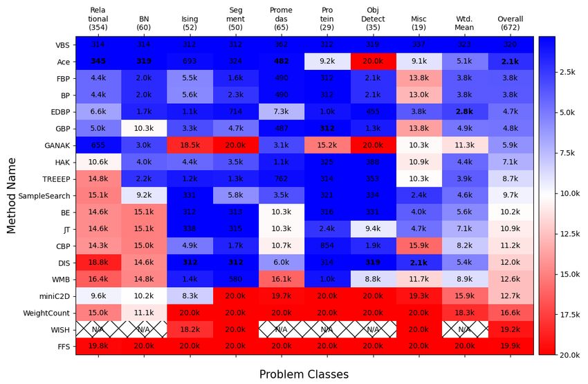
Figure 3: TAP score heatmap - method × problem class
problems in class c. For instance, in ObjDetect class, DIS To name a few, the K* method [Lilien et al., 2005], the A*
has a performance comparable to the Virtual Best Solver. algorithm [Leach and Lemon, 1998], and a method using ran-
Despite the lack of formal guarantees, Belief Propagation domly perturbed MAP solvers [Hazan and Jaakkola, 2012]
and its variants have a low overall TAP score, and a relatively have not been compared due to the unavailability of a suit-
consistent performance across all classes. Thus, BP is the best able implementation. Also, of note are the recently proposed
candidate to perform inference on an assorted dataset if for- techniques for weighted model counting that have shown to
mal guarantees are unnecessary. Among the exact methods, perform well in the model counting competition [Fichte et al.,
Ace performs significantly better than others, and it should be 2020]. Likewise, benchmarks that could not be converted into
preferred for exact inference. compatible formats were not included in the study.
GANAK, a counting-based method performs well on
Relational, Promedas, and BN problems that have a 6 Concluding Remarks and Outlook
higher factor scope size on an average. However, its TAP Several observations are in order based on the extensive em-
scores on the classes with a lower factor scope size such as pirical study: First, observe that the VBS has a mean TAP
Ising, Segment, ObjDetect, and Protein is high, score an order of magnitude lower than the best solver. Such
signaling a poor performance. The opposite is valid for a an observation in the context of SAT solving led to an excit-
subset of methods that do not use model counting, i.e., they ing series of works on the design of portfolio solvers [Hut-
perform well on classes with a smaller factor scope size. The ter et al., 2007; Xu et al., 2008]. In this context, it is worth
methods that show such behavior are JT, BE, and DIS. highlighting that for every problem, at least one method was
able to solve in less than 20 seconds with a 32-factor accu-
5.5 Limitations and Threats to Validity racy. Also, for every benchmark, there existed a technique
The widespread applications of the partition function estima- that could compute an answer with a relative error less than
tion problem have prompted the development of a substan- 20.01 inProceedings of the Thirtieth International Joint Conference on Artificial Intelligence (IJCAI-21)
Survey Track
exciting opportunity for the development of techniques that [Darwiche and Marquis, 2002] Adnan Darwiche and Pierre Mar-
scale better than exact techniques. quis. A knowledge compilation map. Journal of Artificial In-
Finally, the notion of TAP score introduced in this paper telligence Research, 2002.
allows us to compare approximate techniques by consider- [Darwiche, 1995] Adnan Darwiche. Conditioning algorithms for
ing both the estimate quality and the runtime performance. exact and approximate inference in causal networks. In UAI,
We have made the empirical data public, and we invite the 1995.
community to perform a detailed analysis of the behavior [Darwiche, 2001a] Adnan Darwiche. On the tractable counting of
of techniques in the context of structural parameters such as theory models and its application to truth maintenance and belief
treewidth, the community structure of incidence and primal revision. JANCL, 2001.
graphs, and the like. [Darwiche, 2001b] Adnan Darwiche. Recursive conditioning. Ar-
tificial Intelligence, 2001.
Acknowledgments [Darwiche, 2002] Adnan Darwiche. A logical approach to factoring
The authors would like to sincerely thank Adnan Darwiche, belief networks. KR, 2002.
and the anonymous reviewers of IJCAI-20 and AAAI-21 [Darwiche, 2004] Adnan Darwiche. New advances in compiling
for providing detailed, constructive criticism that has signifi- CNF into decomposable negation normal form. In ECAI, 2004.
cantly improved the quality of the paper. [Darwiche, 2009] Adnan Darwiche. Modeling and reasoning with
This work was supported in part by National Research bayesian networks. Cambridge University Press, 2009.
Foundation Singapore under its NRF Fellowship Programme [Darwiche, 2011] Adnan Darwiche. SDD: A new canonical repre-
[NRF-NRFFAI1-2019-0004] and AI Singapore Programme sentation of propositional knowledge bases. In IJCAI, 2011.
[AISG-RP-2018-005], and NUS ODPRT Grant [R-252-000-
[de Colnet and Meel, 2019] Alexis de Colnet and Kuldeep S. Meel.
685-13]. The computational work for this article was per-
Dual hashing-based algorithms for discrete integration. In CP,
formed on resources of the National Supercomputing Centre, 2019.
Singapore (https://www.nscc.sg).
[Dechter et al., 2002] Rina Dechter, Kalev Kask, and Robert Ma-
teescu. Iterative join-graph propagation. In UAI, 2002.
References [Dechter, 1996] Rina Dechter. Bucket elimination: A unifying
[Agrawal et al., 2020] Durgesh Agrawal, Bhavishya, and framework for probabilistic inference. In UAI, 1996.
Kuldeep S. Meel. On the sparsity of xors in approximate [Dechter, 1999] Rina Dechter. Bucket elimination: A unifying
model counting. In SAT, 2020.
framework for reasoning. Artificial Intelligence, 1999.
[Amari et al., 2001] Shun-ichi Amari, Shiro Ikeda, and Hidetoshi
[Doucet et al., 2000] Arnaud Doucet, Nando de Freitas, Kevin
Shimokawa. Information geometry of α-projection in mean field
Murphy, and Stuart Russell. Rao-blackwellised particle filtering
approximation. Advanced Mean Field Methods - Theory and
for dynamic bayesian networks. In UAI, 2000.
Practice, 2001.
[Dudek et al., 2020] Jeffrey M. Dudek, Dror Fried, and Kuldeep S.
[Broka et al., 2018] Filjor Broka, Rina Dechter, Alexander Ihler,
Meel. Taming discrete integration via the boon of dimensionality.
and Kalev Kask. Abstraction sampling in graphical models. In In NeurIPS, 2020.
UAI, 2018.
[Eaton and Ghahramani, 2009] Frederik Eaton and Zoubin Ghahra-
[Chakraborty et al., 2015] Supratik Chakraborty, Dror Fried, mani. Choosing a variable to clamp. In AISTATS, 2009.
Kuldeep S. Meel, and Moshe Y. Vardi. From weighted to
unweighted model counting. In IJCAI, 2015. [Ermon et al., 2011] Stefano Ermon, Carla Gomes, Ashish Sabhar-
wal, and Bart Selman. Accelerated adaptive markov chain for
[Chavira and Darwiche, 2005] Mark Chavira and Adnan Darwiche. partition function computation. In NIPS, 2011.
Compiling bayesian networks with local structure. In IJCAI,
2005. [Ermon et al., 2013a] Stefano Ermon, Carla Gomes, Ashish Sab-
harwal, and Bart Selman. Optimization with parity constraints:
[Chavira and Darwiche, 2007] Mark Chavira and Adnan Darwiche. From binary codes to discrete integration. In UAI, 2013.
Compiling bayesian networks using variable elimination. In IJ-
CAI, 2007. [Ermon et al., 2013b] Stefano Ermon, Carla Gomes, Ashish Sab-
harwal, and Bart Selman. Taming the curse of dimensionality:
[Chavira and Darwiche, 2008] Mark Chavira and Adnan Darwiche. Discrete integration by hashing and optimization. In ICML, 2013.
On probabilistic inference by weighted model counting. Artificial
[Fan and Fan, 2008] Xin Fan and Guoliang Fan. Graphical models
Intelligence, 2008.
for joint segmentation and recognition of license plate characters.
[Chavira et al., 2004] Mark Chavira, Adnan Darwiche, and Man- IEEE Signal Processing Letters, 2008.
fred Jaeger. Compiling relational bayesian networks for exact in-
[Fichte et al., 2020] Johannes K. Fichte, Markus Hecher, and
ference. International Journal of Approximate Reasoning, 2004.
Florim Hamiti. The model counting competition 2020. arXiv
[Choi and Darwiche, 2006] Arthur Choi and Adnan Darwiche. An preprint, 2020.
edge deletion semantics for belief propagation and its practical [Georgiev et al., 2012] Ivelin Georgiev, Ryan H. Lilien, and
impact onapproximation quality. In AAAI, 2006.
Bruce R. Donald. The minimized dead-end elimination criterion
[Cundy and Ermon, 2020] Chris Cundy and Stefano Ermon. Flex- and its application to protein redesign in a hybrid scoring and
ible approximate inference via stratified normalizing flows. In search algorithm for computing partition functions over molecu-
UAI, 2020. lar ensembles. Journal of Computational Chemistry, 2012.
4283Proceedings of the Thirtieth International Joint Conference on Artificial Intelligence (IJCAI-21)
Survey Track
[Gillespie, 2013] Dirk Gillespie. Computing the partition function, [Lauritzen and Spiegelhalter, 1988] S. L. Lauritzen and D. J.
ensemble averages, and density of states for lattice spin systems Spiegelhalter. Local computation with probabilities on graphi-
by sampling the mean. Journal of computational physics, 2013. cal structures and their application to expert systems. Journal of
[Gogate and Dechter, 2005] Vibhav Gogate and Rina Dechter. Ap- the Royal Statistical Society, Series B, 1988.
proximate inference algorithms for hybrid bayesian networks [Leach and Lemon, 1998] Andrew R. Leach and Andrew P. Lemon.
with discrete constraints. In UAI, 2005. Exploring the conformational space of protein side chains using
dead-end elimination and the A* algorithm. Proteins, 1998.
[Gogate and Dechter, 2011] Vibhav Gogate and Rina Dechter.
SampleSearch: Importance sampling in presence of determinism. [Lee et al., 2019] Junkyu Lee, Radu Marinescu, Alexander Ihler,
Artificial Intelligence, 2011. and Rina Dechter. A weighted mini-bucket bound for solving
influence diagrams. In UAI, 2019.
[Grover et al., 2018] Aditya Grover, Tudor Achim, and Stefano Er-
[Lilien et al., 2005] Ryan H. Lilien, Brian W. Stevens, Amy C. An-
mon. Streamlining variational inference for constraint satisfac-
derson, and Bruce R. Donald. A novel ensemble-based scoring
tion problems. In NeurIPS, 2018.
and search algorithm for protein redesign, and its application to
[Hazan and Jaakkola, 2012] Tamir Hazan and Tommi Jaakkola. On modify the substrate specificity of the gramicidin synthetase a
the partition function and random maximum a-posteriori pertur- phenylalanine adenylation enzyme. Journal of Computational
bations. In ICML, 2012. Biology, 2005.
[Henrion, 1988] Max Henrion. Propagating uncertainty in bayesian [Liu and Ihler, 2011] Qiang Liu and Alexander Ihler. Bounding the
networks by probalistic logic sampling. In UAI, 1988. partition function using Holder’s inequality. In ICML, 2011.
[Heskes et al., 2003] Tom Heskes, Kees Albers, and Hilbert Kap- [Liu et al., 2015] Qiang Liu, Jian Peng, Alexander Ihler, and John
pen. Approximate inference and constrained optimization. In Fisher III. Estimating the partition function by discriminance
UAI, 2003. sampling. In UAI, 2015.
[Lou et al., 2017] Qi Lou, Rina Dechter, and Alexander Ihler. Dy-
[Heule et al., 2019] Marijn Heule, Matti Jarvisalo, and Martin
namic importance sampling for anytime bounds of the partition
Suda. Sat competition 2018. Journal on Satisfiability, Boolean
function. In NIPS, 2017.
Modeling and Computation, 2019.
[Ma et al., 2013] Jianzhu Ma, Jian Peng, Sheng Wang, and Jinbo
[Horvitz et al., 1989] Eric J. Horvitz, Jaap Suermondt, and Gre- Xu. Estimating the partition function of graphical models using
gory F. Cooper. Bounded conditioning: Flexible inference for langevin importance sampling. In AISTATS, 2013.
decisions under scarce resources. In UAI, 1989.
[Marinescu, 2019] Radu Marinescu. Merlin: An extensible C++
[Hutter et al., 2007] Frank Hutter, H. Hoos, and Thomas Stutzle. library for probabilistic inference over graphical models, 2019.
Automatic algorithm configuration based on local search. In [Mateescu and Dechter, 1990] Robert Mateescu and Rina Dechter.
AAAI, 2007.
Axioms for probability and belief-function propagation. In UAI,
[Jensen et al., 1990] Finn V. Jensen, Steffen L. Lauritzen, and Kris- 1990.
tian G. Olesen. Bayesian updating in causal probabilistic net- [Mateescu and Dechter, 2005] Robert Mateescu and Rina Dechter.
works by local computation. Computational Statistics Quarterly, AND/OR cutset conditioning. In IJCAI, 2005.
1990.
[McCallum et al., 2009] Andrew McCallum, Karl Schultz, and
[Jerrum and Sinclair, 1993] Mark Jerrum and Alistair Sinclair. Sameer Singh. FACTORIE: Probabilistic programming via im-
Polynomial-time approximation algorithms for the ising model. peratively defined factor graphs. In NIPS, 2009.
SIAM Journal on Computing, 1993. [Meel and Akshay, 2020] Kuldeep S. Meel and S. Akshay. Sparse
[Koller and Friedman, 2009] Daphne Koller and Nir Friedman. hashing for scalable approximate model counting: Theory and
Probabilistic graphical models: Principles and techniques. Adap- practice. In LICS, 2020.
tive Computation and Machine Learning Series, 2009. [Minka, 2001] Thomas P. Minka. A family of algorithms for ap-
[Kschischang et al., 2001] Frank R. Kschischang, Brendan Frey, proximate bayesian inference. PhD Thesis, MIT Cambridge,
and Hans-Andrea Loeliger. Factor graphs and the sum-product 2001.
algorithm. IEEE TIT, 2001. [Molkaraie and Loeliger, 2012] Mehdi Molkaraie and Hans-
[Kuck et al., 2018] Jonathan Kuck, Ashish Sabharwal, and Stefano Andrea Loeliger. Monte carlo algorithms for the partition
Ermon. Approximate inference via weighted rademacher com- function and information rates of two-dimensional channels.
plexity. In AAAI, 2018. IEEE TIT, 2012.
[Mooij, 2010] Joris Mooij. libDAI: A free and open source C++
[Kuck et al., 2019] Jonathan Kuck, Tri Dao, Shengjia Zhao, Burak
library for discrete approximate inference in graphical models.
Bartan, Ashish Sabharwal, and Stefano Ermon. Adaptive hashing
Journal of Machine Learning Research, 2010.
for model counting. In UAI, 2019.
[Murphy, 2012] Kevin Patrick Murphy. Machine learning: a prob-
[Kuck et al., 2020] Jonathan Kuck, Shuvam Chakraborty, Hao abilistic perspective. Probabilistic Machine Learning Series,
Tang, Rachel Luo, Jiaming Song, Ashish Sabharwal, and Stefano 2012.
Ermon. Belief propagation neural networks. In NeurIPS, 2020.
[Oztok and Darwiche, 2015] Umut Oztok and Adnan Darwiche. A
[Lagniez and Marquis, 2017] Jean-Marie Lagniez and Pierre Mar- top-down compiler for sentential decision diagrams. In IJCAI,
quis. An improved decision-DNNF compiler. In IJCAI, 2017. 2015.
[Lagniez and Marquis, 2019] Jean-Marie Lagniez and Pierre Mar- [Pabbaraju et al., 2020] Chirag Pabbaraju, Po-Wei Wang, and
quis. A recursive algorithm for projected model counting. In J. Zico Kolter. Efficient semidefinite-programming based infer-
AAAI, 2019. ence for binary and multi class mrfs. In NeurIPS, 2020.
4284Proceedings of the Thirtieth International Joint Conference on Artificial Intelligence (IJCAI-21)
Survey Track
[Pearl, 1982] Judea Pearl. Reverend bayes on inference engines: A [Wu et al., 2020] Mike Wu, Kristy Choi, Noah Goodman, and Ste-
distributed hierarchical approach. In AAAI, 1982. fano Ermon. Meta-amortized variational inference and learning.
[Pearl, 1986] Judea Pearl. A constraint-propagation approach to In AAAI, 2020.
probabilistic reasoning. In UAI, 1986. [Xu et al., 2008] Lin Xu, Frank Hutter, Holger H. Hoos, and Kevin
Leyton-Brown. SATzilla: Portfolio-based algorithm selection for
[Pearl, 1988] Judea Pearl. Probabilistic reasoning in intelligent sys-
SAT. J. Artif. Intell. Res., 2008.
tems. Networks of Plausible Inference, 1988.
[Yedidia et al., 2000] Jonathan S. Yedidia, William T. Freeman, and
[Peyrard et al., 2019] Nathalie Peyrard, Marie-Josee Cros, Simon
Yair Weiss. Generalized belief propagation. In NIPS, 2000.
de Givry, Alain Franc, Stephane Robin, Regis Sabbadin, Thomas
Schiex, and Matthieu Vignes. Exact or approximate inference in [Zeng et al., 2020] Zhe Zeng, Paolo Morettin, Fanqi Yan, Antonio
graphical models: why the choice is dictated by the treewidth, Vergari, and Guy Van den Broeck. Probabilistic inference with
and how variable elimination can be exploited. ANZJS, 2019. algebraic constraints: Theoretical limits and practical approxima-
tions. In NeurIPS, 2020.
[Qi and Minka, 2004] Yuan Qi and Thomas Minka. Tree-structured
approximations by expectation propagation. In NIPS, 2004. [Zhang and Poole, 1994] Nevin Lianwen Zhang and David Poole.
A simple approach to bayesian network computations. In UAI,
[Roth, 1996] Dan Roth. On the hardness of approximate reasoning. 1994.
Artificial Intelligence, 1996.
[Saeedi et al., 2017] Ardavan Saeedi, Tejas D. Kulkarni, Vikash K.
Mansinghka, and Samuel J. Gershman. Variational particle ap-
proximations. JMLR, 2017.
[Shachter and Peot, 1989] Ross D. Shachter and Mark Alan Peot.
Simulation approaches to general probabilistic inference on be-
lief networks. In UAI, 1989.
[Sharma et al., 2019] Shubham Sharma, Subhajit Roy, Mate Soos,
and Kuldeep S. Meel. GANAK: A scalable probabilistic exact
model counter. In IJCAI, 2019.
[Shu et al., 2018] Rui Shu, Hung Bui, Shengjia Zhao, Mykel
Kochenderfer, and Stefano Ermon. Amortized inference regu-
larization. In NeurIPS, 2018.
[Shu et al., 2019] Rui Shu, Hung Bui, Jay Whang, and Stefano Er-
mon. Training variational autoencoders with buffered stochastic
variational inference. In AISTATS, 2019.
[Soos and Meel, 2019] Mate Soos and Kuldeep S. Meel. BIRD: En-
gineering an efficient CNF-XOR SAT solver and its applications
to approximate model counting. In AAAI, 2019.
[Soos et al., 2020] Mate Soos, Stephan Gocht, and Kuldeep S.
Meel. Tinted, detached, and lazy CNF-XOR solving and its ap-
plications to counting and sampling. In CAV, 2020.
[Thurley, 2006] Marc Thurley. sharpSAT - counting models with
advanced component caching and implicit bcp. In SAT, 2006.
[Viricel et al., 2016] Clement Viricel, David Simonichi, Sophie
Barbe, and Thomas Schiex. Guaranteed weighted counting for
affinity computation: Beyond determinism and structure. In CP,
2016.
[Wainwright et al., 2001] Martin J. Wainwright, Tommi Jaakkola,
and Alan S. Willsky. Tree-based reparameterization for approxi-
mate inference on loopy graphs. In NIPS, 2001.
[Waldorp and Marsman, 2019] Lourens Waldorp and Maarten
Marsman. Intervention in undirected ising graphs and the
partition function. arXiv preprint, 2019.
[Wiegerinck and Heskes, 2003] Wim Wiegerinck and Tom Heskes.
Fractional belief propagation. In NIPS, 2003.
[Winkler, 2002] Gerhard Winkler. Image analysis, random fields
and markov chain monte carlo methods: A mathematical intro-
duction. Stochastic Modelling and Applied Probability, 2002.
[Wu et al., 2019] Mike Wu, Noah Goodman, and Stefano Er-
mon. Differentiable antithetic sampling for variance reduction
in stochastic variational inference. In AISTATS, 2019.
4285You can also read