Magnetar birth: rotation rates and gravitational-wave emission
←
→
Page content transcription
If your browser does not render page correctly, please read the page content below
MNRAS 000, 1–10 (0000)                                               Preprint 7 April 2020              Compiled using MNRAS LATEX style file v3.0

                                              Magnetar birth: rotation rates and gravitational-wave emission

                                              S. K. Lander1,2⋆, D. I. Jones3
                                              1 Schoolof Physics, University of East Anglia, Norwich, NR4 7TJ, U.K.
                                              2 NicolausCopernicus Astronomical Centre, Polish Academy of Sciences, Bartycka 18, 00-716 Warsaw, Poland,
                                              3 Mathematical Sciences and STAG Research Centre, University of Southampton, Southampton SO17 1BJ, U.K.
arXiv:1910.14336v2 [astro-ph.HE] 5 Apr 2020

                                              7 April 2020

                                                                                    ABSTRACT
                                                                                    Understanding the evolution of the angle χ between a magnetar’s rotation and magnetic axes
                                                                                    sheds light on the star’s birth properties. This evolution is coupled with that of the stellar
                                                                                    rotation Ω, and depends on the competing effects of internal viscous dissipation and external
                                                                                    torques. We study this coupled evolution for a model magnetar with a strong internal toroidal
                                                                                    field, extending previous work by modelling – for the first time in this context – the strong
                                                                                    proto-magnetar wind acting shortly after birth. We also account for the effect of buoyancy
                                                                                    forces on viscous dissipation at late times. Typically we find that χ → 90◦ shortly after
                                                                                    birth, then decreases towards 0◦ over hundreds of years. From observational indications that
                                                                                    magnetars typically have small χ, we infer that these stars are subject to a stronger average
                                                                                    exterior torque than radio pulsars, and that they were born spinning faster than ∼ 100 − 300 Hz.
                                                                                    Our results allow us to make quantitative predictions for the gravitational and electromagnetic
                                                                                    signals from a newborn rotating magnetar. We also comment briefly on the possible connection
                                                                                    with periodic Fast Radio Burst sources.
                                                                                    Key words: stars: evolution – stars: interiors – stars: magnetic fields – stars: neutron – stars:
                                                                                    rotation

                                              1 INTRODUCTION                                                               detectable gravitational waves (GWs) (Cutler 2002; Stella et al.
                                                                                                                           2005; Dall’Osso et al. 2009; Kashiyama et al. 2016), though signal-
                                              Magnetars contain the strongest long-lived magnetic fields known
                                                                                                                           analysis difficulties (Dall’Osso et al. 2018) make it particularly im-
                                              in the Universe. Unlike radio pulsars, the canonical neutron stars
                                                                                                                           portant to have realistic templates of the evolving star. As we will see
                                              (NSs), magnetars do not have enough rotational energy to power
                                                                                                                           later, detection of such a signal would provide valuable constraints
                                              their emission, and so the energy reservoir must be magnetic
                                                                                                                           on the star’s viscosity (i.e. microphysics) and internal magnetic
                                              (Thompson & Duncan 1995). Through sustained recent effort in
                                                                                                                           field.
                                              modelling, we now have a reasonable idea of the physics of the
                                              observed mature magnetars.
                                                    The early life of magnetars is far more poorly understood,
                                              although models of various phenomena rely on them being born                       A major weakness in all these models is the lack of convinc-
                                              rapidly rotating. Indeed, the very generation of magnetar-strength           ing observational evidence for newborn magnetars with such fabu-
                                              fields is likely to involve one or more physical mechanisms that              lously high rotation rates; the galactic magnetars we observe have
                                              operate at high rotation frequencies f : a convective dynamo                 spun down to rotational periods P ∼ 2 − 12 s (Olausen & Kaspi
                                              (Thompson & Duncan 1993) and/or the magneto-rotational insta-                2014), and heavy proto-magnetars formed through binary inspi-
                                              bility (Rembiasz et al. 2016). Uncertainties about how these ef-             ral may since have collapsed into black holes. Details of mag-
                                              fects operate at the ultra-high electrical conductivity of proto-            netar birth are, therefore, of major importance. In this paper
                                              NS matter – where the crucial effect of magnetic reconnection                 we show that an evolutionary model of magnetar inclination an-
                                              is stymied – could be partially resolved with constraints on the             gles – including, for the first time, the key effect of a neutrino-
                                              birth f of magnetars. In addition, a rapidly-rotating newborn mag-           driven proto-magnetar wind – allows one to infer details about
                                              netar could be the central engine powering extreme electromag-               their birth rotation, GW emission, and the prospects for accom-
                                              netic (EM) phenomena – superluminous supernovae and gamma-                   panying EM signals. Furthermore, two potentially periodic Fast
                                              ray bursts (GRBs) (Thompson et al. 2004; Kasen & Bildsten 2010;              Radio Burst (FRB) sources have very recently been discovered
                                              Woosley 2010; Metzger et al. 2011). Such a source might also emit            (The CHIME/FRB Collaboration et al. 2020; Rajwade et al. 2020),
                                                                                                                           which may be powered by young precessing magnetars (Levin et al.
                                                                                                                           2020; Zanazzi & Lai 2020); we show that our work allows con-
                                              ⋆   samuel.lander@uea.ac.uk                                                  straints to be put on such models.

                                              © 0000 The Authors
2      S. K. Lander and D. I. Jones
2 MAGNETAR EVOLUTION
We begin by outlining the evolutionary phases of interest here. We
consider a magnetar a few seconds after birth, once processes related
to the generation and rearrangement of magnetic flux have probably
saturated. The physics of each phase will be detailed later.
      Early phase (∼ seconds): the proto-NS is hot and still par-
tially neutrino-opaque. A strong particle wind through the evolving
magnetosphere removes angular momentum from the star. Bulk
viscosity – the dominant process driving internal dissipation – is
suppressed.
      Intermediate phase (∼ minutes–hours): now transparent to neu-
trinos, the star cools rapidly, and bulk viscosity turns on. The wind is
now ultrarelativistic, and the magnetospheric structure has settled.
      Late phase (∼ days and longer): the presence of buoyancy
forces affects the nature of fluid motions within the star, so that they
are no longer susceptible to dissipation via bulk viscosity. The star
slowly cools and spins down.                                                Figure 1. Interior and exterior field of a newborn magnetar. Poloidal-field
                                                                            lines are shown in blue; the internal toroidal field (directed perpendicular
                                                                            to the page) is located in the red shaded region. The exterior field geometry
2.1 Precession of the newborn, fluid magnetar                               and the star’s spindown depend on the rotation and magnetic-field strength.
                                                                            The open-field line region of the magnetosphere, with opening half-angle
Straight after birth, a magnetar (sketched in Fig. 1) is a fluid body; its
                                                                            θop , begins at a line joining to an equatorial current sheet at the Y -point,
crust only freezes later, as the star cools. Normally, the only steady      located at a radius RY from Ω. Both RY and the Alfvén radius R A evolve
motion that such a fluid body can sustain is rigid rotation about one        in time towards the light-cylinder radius R L , with RY ≤ R A ≤ R L .
axis Ω. However, the star’s internal magnetic field1 Bint provides a
certain ‘rigidity’ to the fluid, manifested in the fact that it can induce   capture the complex physics of the newborn magnetar as faithfully
some distortion ǫB to the star (Chandrasekhar & Fermi 1953). For            as possible. In attempting to do so, our calculation will resort to
a dominantly poloidal Bint this distortion is oblate; whereas a dom-        a number of approximations and parameter-space exploration of
inantly toroidal Bint induces a prolate distortion. If the magnetic         uncertain quantities. Nonetheless, as we will discuss at the end, we
axis B is aligned with Ω, the magnetic and centrifugal distortions          believe our conclusions are generally insensitive to this uncertainties
will also be aligned, and the stellar structure axisymmetric and sta-       – and that confronting these issues is better than ignoring them.
tionary – but if they are misaligned by some angle χ, the primary
rotation about Ω will no longer conserve angular momentum; a slow
secondary rotation with period                                              2.2 The evolving magnetar magnetosphere
             2π                                                             The environment around a NS determines how rapidly it loses an-
Pprec =                                                              (1)
          ΩǫB cos χ                                                         gular momentum, and hence spins down. This occurs even if the
                                                                            exterior region is vacuum, through Poynting-flux losses at a rate
about B is also needed. These two rotations together constitute
                                                                            (proportional to sin2 χ) which may be solved analytically (Deutsch
rigid-body free precession, but since the star is fluid this bulk
                                                                            1955). The vacuum-exterior assumption is still fairly frequently em-
precession must be supported by internal motions (Spitzer 1958;
                                                                            ployed in the pulsar observational literature, although it exhibits the
Mestel & Takhar 1972). The first self-consistent solution for these
                                                                            pathological behaviour that spin-down decreases as χ → 0◦ and
motions, requiring second-order perturbation theory, was only re-
                                                                            ceases altogether for an aligned rotator ( χ = 0◦ ).
cently completed (Lander & Jones 2017).
                                                                                  The magnetic-field structure outside a NS, and the associated
      On secular timescales these internal motions undergo vis-
                                                                            angular-momentum losses, change when one accounts for the dis-
cous damping, and the star is subject to an external EM torque
                                                                            tribution of charged particles that will naturally come to populate
(Mestel & Takhar 1972; Jones 1976). The latter effect tends to drive
                                                                            the exterior of a pulsar (Goldreich & Julian 1969). Solving for the
χ → 0◦ , as recently explored by Şaşmaz Muş et al. (2019) in the
                                                                            magnetospheric structure is now analytically intractable, but numer-
context of newborn magnetars; and if the star’s magnetic distortion
                                                                            ical force-free solutions for the cases of χ = 0◦ (Contopoulos et al.
is oblate, viscous damping of the internal motions supporting pre-
                                                                            1999) and χ , 0◦ (Spitkovsky 2006) demonstrate a structure similar
cession also causes χ to decrease. Viscous damping of a prolate
                                                                            to that sketched in Fig. 1: one region of closed, corotating equatorial
star (i.e. one with a dominantly toroidal Bint ) is more interesting: it
                                                                            field lines and another region of ‘open’ field lines around the polar
drives χ → 90◦ , and thus competes with the aligning effect of the
                                                                            cap. The two are delineated by a separatrix: a cusped field line that
exterior torque. Therefore, whilst it is not obvious how the inter-
                                                                            joins an equatorial current sheet at the Y-point RY . Corotation of
nal motions could themselves be directly visible, the effect of their
                                                                            particles along magnetic fields ceases to be possible if their linear
dissipation may be.
                                                                            velocity exceeds the speed of light; this sets the light cylinder radius
      In our previous paper, Lander & Jones (2018), we presented
                                                                            RL = c/Ω. In practice, simulations employing force-free electro-
the first study of the evolution of χ including the competing effects
                                                                            dynamics find magnetospheric structures with RY = RL , although
of the exterior torque and internal dissipation. The balance between
                                                                            solutions with RY < RL are not, a priori, inadmissible. The angular-
these effects was shown to be delicate – and so it is important to
                                                                            momentum losses from these models proved to be non-zero in the
                                                                            case χ = 0◦ , in contrast with the vacuum-exterior case. These losses
1  Later on we will use Bint more precisely, to mean the volume-averaged    again correspond to the radiation of Poynting flux, but are enhanced
internal magnetic-field strength.                                            compared with the vacuum case, since there is now additional work

                                                                                                                              MNRAS 000, 1–10 (0000)
Magnetar rotation and GWs                    3
done on the charge distribution outside the star (Timokhin 2006).              earlier results are taken on trust; we denote some equation X taken
Results from these simulations should be applicable in the ultra-              from M11 by (M11;X).
relativistic wind limit, and since it appears RY = RL generically                    To avoid cluttering what follows with mass and radius factors,
for this case, the losses are also independent of any details of the           we report equations and results for our fiducial magnetar model
magnetospheric structure.                                                      with R∗ = 12 km and a mass 1.4M ⊙ . We have, however, performed
      Shortly after birth, however, a magnetar exterior is unlikely to         simulations with a 15-km radius, 2.4M ⊙ model, as a crude ap-
bear close resemblance to the standard pulsar-magnetosphere mod-               proximation to a massive magnetar formed through binary inspiral
els. A strong neutrino-heated wind of charged particles will carry             (Giacomazzo & Perna 2013), finding similar results.
angular momentum away from the star (Thompson et al. 2004) – a                       We start from the established mass-loss rate MÛ ν
concept familiar from the study of non-degenerate stars (Schatzman             (Qian & Woosley 1996) of a non-rotating, unmagnetised proto-NS:
1962) – and these losses may dominate over those of Poynting-flux                                                       5/3
                                                                                                                 Lν             Eν 10/3
type. At large distances from the star, a particle carries away more           MÛ ν = −6.8 × 10⁻⁵ M ⊙ s−1 52                             ,      (3)
angular momentum than if it were decoupled from the star at the                                             10 erg s−1        10 MeV
stellar surface. At sufficient distance, however, there will be no ad-           where M ⊙ is the solar mass and Lν and Eν are the neutrino luminos-
ditional enhancement to angular momentum losses as the particle                ity and energy per neutrino, respectively. The idea will be to adjust
moves further out; the wind speed exceeds the Alfvén speed, mean-              this result to account for the effects of rotation and a magnetic field.
ing the particle cannot be kept in corotation with the star. The radius        From the simulations of Pons et al. (1999) (see M11 Fig. A1), we
at which the two speeds become equal is the Alfvén radius R A.                 make the following fits to the evolution of Lν and Eν :
      An additional physical mechanism for angular-momentum loss
becomes important at rapid rotation: as well as thermal pressure,                    Lν                      t [s]                t [s] 4
                                                                                               ≈ 0.7 exp   −         + 0.3   1 −          ,
a centrifugal force term assists in driving the particle wind. Each            1052 erg s−1                   1.5                  50
escaping particle then carries away an enhanced amount of angular
                                                                                       Eν                    t [s]          t [s]
momentum (Mestel 1968a; Mestel & Spruit 1987). The mechanism                                   ≈ 0.3 exp −           +1−          .               (4)
                                                                                     10 MeV                    4             60
is active up to the sonic radius Rs = (GM/Ω2 )1/3 , at which these
centrifugal forces are strong enough to eject the particle from its            Our model does not allow for evolution of the radius R∗ , so our time
orbit. If it is still in corotation with the star until the point when it is   zero corresponds to two seconds after bounce, at which point R∗
centrifugally ejected, i.e. R A ≥ Rs , the maximal amount of angular           has stabilised at ∼ 12 km.
momentum is lost.                                                                   Charged particles can only escape the magnetised star along
      Another source of angular-momentum losses is plausible in                the fraction of open field lines, so the original mass-loss rate (3)
the aftermath of the supernova creating the magnetar: a magnetic               should be reduced to MÛ = MÛ ν Fop , where (M11;A4)
torque from the interaction of the stellar magnetosphere with fall-                                          h       p        i
                                                                               Fop = 1 − cos(θ op ) = 1 − cos arcsin R∗ /RY .                     (5)
back material. The physics of this should resemble that of the classic
problem of a magnetic star with an accretion disc (Ghosh & Lamb                                         √
                                                                               Now since cos(arcsin x) = 1 − x 2 , we have
1978), but the dynamical aftermath of the supernova is far messier,
                                                                                        p
and results will be highly sensitive to the exact physical conditions          Fop = 1 − 1 − R∗ RLY /RL ,                                         (6)
of the system. Attempting to account for fallback matter would
therefore not make our model any more quantitatively accurate.                 where RLY ≡ RL /RY . When f & 500 Hz, the mass loss may
      We recall that there are four radii of importance in the                 experience a centrifugal enhancement Fcent > 1, so that (M11;A15):
magnetar-wind problem. Two of them, RL and Rs , depend only                    MÛ = MÛ ν Fop Fcent .                                              (7)
on the stellar rotation rate. The others are RY , associated with elec-
tromagnetic losses, and R A , associated with particle losses. We will         Our approach will be first to ignore this to obtain a slow-rotation
need to account for how these quantities, which both grow until                solution, which we then use to calculate Fcent (and hence the gen-
                                                                                     Û ‘perturbatively’. We start by combining equations (6) and
                                                                               eral M)
reaching RL , evolve over the early phase of the magnetar’s life. Fi-
nally, we also need to know, at a given instant, the dominant physics          (2) (with Fcent = 1) to get a relation between RLY and σ0 . But
governing the star’s angular-momentum loss. This is captured in the            another, phenomenological relation RLY = max{(0.3σ00.15 )−1, 1}
wind magnetisation σ0 , the ratio of Poynting-flux to particle kinetic          (Bucciantini et al. 2006; Metzger et al. 2007) also links the two. The
energy losses:                                                                 relations may therefore be combined to eliminate σ0 :
                                                                                     r              !
        2 F 2 R 4 Ω2
       Bext op ∗
                                                                                           R∗          1/0.15   0.3−1/0.15 c3 MÛ ν
σ0 =                 ,                                                  (2)     1− 1−          RLY RLY        =       2 R 4 Ω2
                                                                                                                                   .               (8)
            Û 3                                                                            RL                       Bext  ∗
            Mc
where Fop is the fraction of field lines which remain open beyond               This equation may be solved to find RLY for given Bext, Ω and t.
RY (see Fig. 1) and Bext is the surface field strength. Note that the           It has real solutions as long as R∗ /RY < 1; the Y -point cannot be
limits σ0 ≪ 1 (σ0 ≫ 1) correspond to non(ultra)-relativistic winds.            within the star. As RY → R∗ all magnetospheric field lines become
     At present there are neither analytic nor numerical solutions             open, and the following limits are attained:
providing a full description of the proto-magnetar wind. In the ab-                                           2 R4 Ω2 /( M
                                                                                                                         Û ν c3 ).
                                                                               RLY = RL /R∗ , Fop = 1 , σ0 = Bext ∗                               (9)
sence of these, we will adapt the model of Metzger et al. (2011)
(hereafter M11), which at least attempts to incorporate, semi-                 Accordingly, in cases where equation (8) has no real solutions, we
quantitatively, the main ingredients that such a full wind solution            use the above limiting values.
should have. Based on their work, we have devised a simplified                       Next we move on to calculate the centrifugal enhancement. As
semi-analytic model for the magnetar wind, capturing the same                  discussed earlier, this depends strongly on the location of R A with
fundamental wind physics but more readily usable for our simula-               respect to Rs . Only the former quantity depends on the magneto-
tions. Our description of the details is brief, but self-contained if          spheric physics, and as for the Y-point location we find it convenient

MNRAS 000, 1–10 (0000)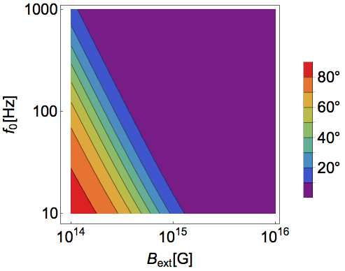
4 S. K. Lander and D. I. Jones
f[Hz] f[] f[H]
1000 1
800 3
600
4
400 9 1
2
t[s] t[s] t[s]
20 40 60 80 20 40 60 80 20 40 60 80
Figure 2. The first 80 s of rotational evolution for different model newborn magnetars, with fixed χ and (from left to right): f0 = 1 kHz, Bext = 1016 G;
f0 = 100 Hz, Bext = 1016 G; f0 = 1 kHz, Bext = 1015 G. Linestyles 1,2 show (respectively) χ = 0, 90◦ models evolved with the magnetar wind prescription
described in section 2.2 for 40 s and thereafter with a ‘pulsar’ prescription (third line of equation (12)); linestyles 3,4 show the corresponding results using the
‘pulsar’ prescription from birth. Note that before 40 s, lines 1 and 2 become indistinguishable from one another for higher f0 and Bext .
to work with the dimensionless radius RL A ≡ RL /R A. Now, M11 the two limiting regimes over a timescale short compared with the
−1/3 evolution of both χ and Ω.
employ the phenomenological relation RL A = max{σ0 , 1}; we
therefore just need to find σ0 . To do so, we use the solution we have Fig. 2 shows sample evolutions, comparing the magnetar wind
just obtained for RLY , plugging it in equation (7) to make a first prescription with one often used for pulsars (and also used, with
calculation of MÛ in the absence of any centrifugal enhancement (i.e. a slightly different numerical prefactor, in Lander & Jones (2018)).
setting Fcent = 1), then using the result in equation (2) to find σ0 . For the extreme case of f0 = 1 kHz, Bext = 1016 G (left-hand
We may now calculate the centrifugal enhancement: panel), we see that the rotation rate has roughly halved after 40 s
max
for all models – although the most rapid losses are suffered by the
Fcent = Fcent [1 − exp(−R A/Rs )] + exp(−R A/Rs ), (10) model with χ = 90◦ and the pulsar prescription. For less extreme
where (M11;A12,A13) cases (middle and right panels), however, the magnetar wind always
" gives the greatest losses. Finally, as expected from equation (12),
1.5 #
max f [kHz] we see that the value of χ often has less effect on the magnetar-wind
Fcent = exp (11) losses than those from the pulsar prescription.
2.8 max{sin(θ op ), sin χ}
is the maximum possible enhancement factor to the mass loss,
occurring when R A ≥ Rs . 2.3 Buoyancy forces
The centrifugal enhancement relies on particles reaching large
distances from Ω whilst remaining in corotation; we can see this will At a much later stage, another physical effect needs to be modelled,
not happen if open field lines remain close to this axis out to large related to the role of buoyancy forces on internal motions.
distances. As a diagnostic of this, M11 assume that enhancement The proportions of different particles in a NS varies with depth.
will not occur if a typical open-field line angle ( χ + θ op ) ≪ π/2, If one moves an element of NS matter to a different depth, chem-
but will do if ( χ + θ op ) & π/2. In practice we have to decide on ical reactions act to re-equilibrate it with its surroundings, on a
an angle delineating the two regimes: we take π/4. Accordingly, we timescale τchem . When the temperature T is high, τchem ≪ Pprec ,
will adopt equation (7) for the full mass-loss rate, but set Fcent = 1 so moving fluid elements are kept in chemical equilibrium. Once
when χ + θ op < π/4. We now re-calculate equation (2) to find the the star has cooled sufficiently, however, reactions will have slowed
full σ0 , and so the EM energy-loss rate (M11;A5): down enough for fluid elements to retain a different composition
from their surroundings (Lander & Jones 2018); they will there-
Û 2/3
c2 Mσ σ0 < 1 and t < 40s fore be subject to a buoyancy force due to the chemical gradient
2 2 0
EÛEM = 3 c Mσ Û 0 σ0 ≥ 1 and t < 40s (12) (Reisenegger & Goldreich 1992). This force tends to suppress ra-
R 2 dial motion, and hence will predominantly affect the compressible
− ∗ Ω4 B 2 (1 + sin2 χ)
t ≥ 40s.
4c3 ext piece of the motions (Mestel & Takhar 1972; Lasky & Glampedakis
Within one minute, the bulk of the star’s neutrinos have escaped 2016). For this phase, one would ideally generalise the lengthy cal-
and so the proto-magnetar wind weakens greatly. Here we take the culation of Lander & Jones (2017) to include buoyancy forces, but
wind to be negligible after 40 s, at which point we switch to a this is very likely to be intractable. In lieu of this, we will simply
fit (Spitkovsky 2006) to numerical simulations of pulsar magneto- impose that the motions become divergence-free below some tem-
spheres, corresponding to the ultrarelativistic limit of the wind (i.e. perature Tsolen , which we define to be the temperature for which
kinetic losses being negligible). For all our models σ0 becomes
large and RY → RL before the 40-second mark at which we switch −6
T ρ̄ 2/3
to this regime; see M11 for more details. Pprec = τchem = 0.2 , (13)
109 K ρnuc
Note that the first and second lines of equation (12) are formally
correct only in the limits σ0 ≪ 1 and σ0 ≫ 1, respectively, with no taking the expression for τchem from Reisenegger & Goldreich
such simple expressions existing for the case σ0 ∼ 1. Treating the (1992), and where ρnuc is nuclear density and ρ̄ the average core
latter case is beyond the scope of the present work, so we simply density. Tsolen is clearly a function of Bint and Ω; its typical value is
switch between the first two regimes of equation (12) at σ0 = 1. We 109 − 1010 K. For T < Tsolen , bulk viscous dissipation (depending
do not expect this to introduce any serious uncertainty in our work, on the compressibility of the internal motions) therefore becomes
however: the wind magnetisation makes a rapid transition between redundant, and we shut it off in our evolutions, leaving only the
MNRAS 000, 1–10 (0000)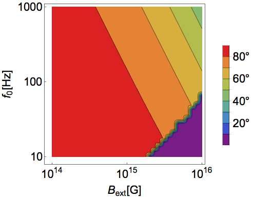
Magnetar rotation and GWs                     5
ineffective shear-viscous dissipation. Without significant viscous             interplay between viscous dissipation EÛvisc of internal fluid motions,
damping, the star’s proclivity towards becoming an orthogonal ro-            and external torques:
tator ( χ = 90◦ ) is suppressed.                                                                          (χ)
      Our evolutionary model employs standard fluid physics, and                            EÛvisc       EÛEM
                                                                             χÛ =                     +       .                                (16)
cannot therefore describe any effects related to the gradual forma-                  IǫB sin χ cos χΩ2    IΩ2
tion of the star’s crust. The star’s motion depends on distortions
                                                                             Now, χÛ should vanish for χ = 0◦, 90◦ (Mestel 1968b). The EÛEM
misaligned from the rotation axis; at late stages this may include, or
                                                                             from equation (12) does not satisfy this, however; it represents the
even be dominated by, elastic stresses in the crust. For the magnetar-
                                                                             spindown part of the full external torque, whereas χÛ depends on a
strength fields we consider, however, it is reasonable to assume that
                                                                             torque component orthogonal to this. As a simple fix that gives the
magnetic distortions dominate. Our fluid model of a magnetar’s χ-                                                           (χ)
evolution should predict the correct long-timescale trend, even if it        correct limiting behaviour of χ, Û we take EÛEM = sin χ cos χ EÛEM
cannot describe short-timescale seismic features (see discussion).           for t < 40 s. For the later phase, Philippov et al. (2014) suggest the
      Finally, as the star cools the core will form superfluid compo-         expression
nents, and the interaction between these may provide a new cou-                        R2
                                                                                (χ)
pling mechanism between the rotation and magnetic-field evolution             EÛEM = ∗3 Ω4 Bext   2
                                                                                                    k sin χ cos χ,                             (17)
                                                                                       4c
(Ruderman et al. 1998). It is not clear what effect – if any – this will
have on the long-timescale evolution of χ.                                   based on fits to numerical simulations, and finding k ≈ 1 for dipo-
                                                                             lar pulsar magnetospheres. This is a sensible result, since setting
                                                                             k = 1 in equation (17) gives the analytic result for the case of a
                                                                             vacuum exterior. Evolutions for a vacuum exterior were performed
3 EVOLUTION EQUATIONS                                                        in Lander & Jones (2018); we also considered pulsar-like models,
We follow the coupled Ω − χ evolution of a newborn magnetar                  but with an alignment torque that did not vanish as χ → 0◦ . The
with a strong, large-scale toroidal Bint in its core – the expected out-     present treatment improves upon this.
come of the birth physics (Jones 1976; Thompson & Duncan 1993).                     Although equation (17) reflects the physics of pulsar magne-
For stability reasons (Tayler 1980) this must be accompanied by a            tospheres, the coronae of magnetars have a different physical origin
poloidal-field component, but we will assume that within the star             and are likely to be complex multipolar structures, which will in
it is small enough to be ignored here (it also retains consistency           turn affect the alignment torque. Furthermore, there are hints that
with the solution we have for the internal motions; Lander & Jones           a magnetar corona may lead to an enhanced torque, k > 1, com-
(2017)). We assume there is no internal motion, and hence no dis-            pared with the pulsar case (Thompson et al. 2002; Younes et al.
sipation, in the outer envelope (the region that becomes the crust           2017). On the other hand, for relatively modest magnetic fields
once the star has cooled sufficiently).                                        (B ∼ 1014 G) these coronae are likely to be transient features
      One unrealistic feature of purely toroidal fields is that Bext = 0.     (Beloborodov & Thompson 2007; Lander 2016); whilst we may still
As in Lander & Jones (2018), we will assume that the poloidal-field           think of k as embodying the long-term average torque, it therefore
component – negligible within the star – becomes significant as one           seems implausible for the appropriate value of k to be far larger than
moves further out, and links to a substantial Bext sharing the same          unity. In the absence of suitable quantitative results for magnetars,
symmetry axis as Bint . We then express the magnetic ellipticity as:         here we will simply adopt equation (17) to describe the alignment,
                                                                             but explore varying the torque prefactor k to check how strong the
                                                2
                    Bint 2               −4 Bint         Bext 2              alignment torque needs to be for consistency with the model.
ǫB = −3× 10−4                 =  −3× 10                           , (14)
                   1016 G                     Bext      1016 G                      Finally, the gravitational radiation reaction torque on the star
                                                                             – like its electromagnetic counterpart – has an aligning effect on
where the first equality comes from self-consistent solutions of              the B and Ω axes. It is given by a straightforward expression that
the star’s hydromagnetic equilibrium (Lander & Jones 2009) with a
                                                                             could be included in our evolutions; we neglect it, however, as one
purely toroidal internal field, and the second equality links this el-
                                                                             can easily show that the GW energy losses (Cutler & Jones 2001)
lipticity to the exterior field strength (somewhat arbitrarily) through       in (15) and (16) are always negligible compared with EÛEM for the
the ratio Bext /Bint . Note that the negative sign of ǫB indicates that
                                                                             models we consider. For instance, for a star with Bext = 1016 G and
the distortion is prolate.
                                                                              f = 1 kHz, the ratio of GW-driven spindown to EM Poynting-type
      A typical model encountered in the literature (e.g. Stella et al.      spindown is ∼ 10−4 . This ratio scales as f 2 Bint4 /B 2 , so would be
(2005)) assumes a ‘buried’ magnetic field, with Bext /Bint ≪ 1, al-                                                                  ext
                                                                             even smaller for more slowly spinning and less strongly magnetised
though self-consistent equilibrium models with vacuum exteriors
                                                                             stars. Furthermore, we have not considered the torque enhancement
have Bext ∼ Bint (Lander & Jones 2009). The results for f and χ              due to the magnetar wind, which would further reduce the ratio.
vary little with the choice of this ratio, since it is mostly the exterior
                                                                                    Viscosity coefficients have strong T-dependence, so this should
torque, i.e. Bext , that dictates the last-phase evolution, and we there-
                                                                             also be accounted for. We assume an isothermal stellar core (recall
fore set the ratio to unity for simplicity unless stated otherwise – an      that we do not consider dissipation in the envelope/crust) with
upper limit for our model, as Bext /Bint & 1 would be inconsistent                        (
with the toroidal field dominating within the star. Only in section 6            T(t)        40 − 3940 t[s]              t ≤ 40 s,
do we explore varying this ratio, as the predicted gravitational and             10
                                                                                       =                           −1/6                        (18)
                                                                             10 K           [1 + 0.06(t[s] − 40)]       t > 40 s,
electromagnetic emission are affected by the relative strength of the
magnetic field inside and outside the star.                                   which mimics the differing cooling behaviour in the neutrino diffu-
      The Ω-evolution is given by the simple, familiar expression:           sion and free-streaming regimes, with the latter expression coming
                                                                             from Page et al. (2006). The isothermal assumption is indeed quite
    Û
Û = EEM ,
Ω                                                                    (15)    reasonable for the latter case, though less so for the former (see,
     IΩ                                                                      e.g., Pons et al. (1999)); the temperature may vary by a factor of a
where I is the moment of inertia, whilst the χ-evolution involves an         few in the core at very early times.

MNRAS 000, 1–10 (0000)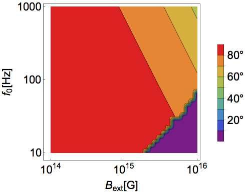
6      S. K. Lander and D. I. Jones
                                                                                              1000

                                                                                               100                                               90°


                                                                                       ]
                                                                                                10                                               60°


                                                                                                                                                       χ
                                                                                       f[
                                                                                                    1                                            30°
                                                                                                                                                 0°
                                                                                               0
                                                                                                        1   100     104    106        108
                                                                                                                      t[s]
                                                                                              ,-.                                                90°

                                                                                          5

                                                                                       ]
                                                                                          2

                                                                                                                                                       χ
                                                                                               *+                                                60°

                                                                                       f[
Figure 3. Distribution of inclination angles (colourscale) after one day, for a
range of f0 and Bext as shown, and with χ0 = 1◦ for all models. All models
in the considered parameter range have already reached either the aligned-
or orthogonal-rotator limit, though the orthogonal rotators will all start to                                                                    3/°
align at later times.                                                                                       !"#    $%4        &'6     ()8
                                                                                                                       t[s]
      In calculating the viscous energy losses EÛvisc we assume the
same well known forms for shear and bulk viscosity as described in                Figure 4. Evolution of f (solid line) and χ (dashed line) for two magnetars.
Lander & Jones (2018). Whilst shear viscosity is always assumed to                Top: f0 = 1 kHz, Bint = Bext = 1016 G, bottom: f0 = 100 Hz, Bint =
be active (albeit inefficient), bulk viscosity is not. We have already              Bext = 1014 G. For illustrative purposes χ0 = 30◦ is chosen, but a smaller
discussed why we take it to be inactive at late times when T < Tsolen ,           value is more likely. For both models χ decreases for the first ∼ 40 s, then
but it is also suppressed in the early era, whilst the proto-neutron star         increases rapidly to 90◦ as bulk viscosity becomes active, staying there until
matter is still partially neutrino-opaque and reactions are inhibited.            the internal motions become solenoidal (at t ∼ 103 s for the left-hand model;
Following Lai (2001), we will switch on bulk viscosity once the                   at t ∼ 108 s for the right-hand one), after which the spindown torque is able,
temperature drops below 3 × 10¹⁰ K. Note that while we include                    slowly, to drive χ back towards 0◦ .
the viscosity mechanisms traditionally considered in such analyses
as ours, other mechanisms can act. Of possible relevance in the
very early life of our star is the shear viscosity contributed by the
                                                                                  with χ ≈ 0◦ . If rapid rotation drives magnetic-field amplification,
neutrinos themselves (see e.g. Guilet et al. (2015)). We leave study
                                                                                  however, a real magnetar born with such a low f could not reach
of this to future work, merely noting for now that its inclusion would
                                                                                  B ∼ 1016 G.
increase the tendency for our stars to orthogonalise.
                                                                                       Fig. 4 shows the way f and χ evolve, for all models in our
      Whatever its microphysical nature, viscous dissipation acts
                                                                                  parameter space except the aligned rotators of Fig. 3: an early phase
on the star’s internal fluid motions, for which we use the only self-
                                                                                  of axis alignment, rapid orthogonalisation, then slow re-alignment.
consistent solutions to date (Lander & Jones 2017). We do not allow
                                                                                  The evolution for most stars in our considered parameter range is
for any evolution of Bint .
                                                                                  similar, though proceeds more slowly for lower Bint , Bext and f0 , as
                                                                                  seen by comparing the left- and right-hand panels (see also Fig. 5
                                                                                  and 6).
4 SIMULATIONS
We solve the coupled Ω − χ equations (15) and (16) with the physi-
cal input discussed above. The highly coupled and non-linear nature
of the equations means that numerical methods are required, and
we therefore use adapted versions of the Mathematica notebooks
                                                                                  5 COMPARISON WITH OBSERVATIONS
described in detail in Lander & Jones (2018). Only in a few limits
are analytic results possible, e.g. at late times where χ has reduced             Next we compare our model predictions with the population of
to nearly zero (see below), and the spin-down then proceeds as the                observed magnetars. Typical magnetars have P ∼ 2 − 12 s and
familiar power-law solution to equation (12). Unless stated other-                Bext ∼ 1014 − 1015 G; comparing these values with Fig. 5, we see
wise, we start all simulations with a small initial inclination angle,            that they are consistent with the expected ages of magnetars, roughly
χ0 ≡ χ(t = 0) = 1◦ .                                                              1000 − 5000 yr (see, e.g., Tendulkar et al. (2012)). The results in
      Fig. 3 shows the distribution of χ after one day, for our                   Fig. 5 are virtually insensitive to the exact value of the alignment-
chosen newborn-magnetar parameter space f0 ≡ f (t = 0) =                          torque prefactor k (we take k = 2 in these plots). The model results
10 − 103 Hz, Bext = 1014 − 1016 G and with k = 2. This is sim-                    are very similar for different Bint and χ0 , and the vertical contours
ilar to our earlier results (Lander & Jones 2018), where the effect                show that present-day periods are set primarily by Bext , and give no
of buoyancy forces on interior motions was not considered. As the                 indication of the birth rotation.
orthogonalising effect of internal viscosity becomes suppressed, the                     Observations contain more information than just P and the
orthogonal rotators can be expected to start aligning at later times,             inferred Bext , however. The four magnetars observed in radio
whilst the small region of aligned rotators will obviously remain                 (Olausen & Kaspi 2014):

                                                                                                                                    MNRAS 000, 1–10 (0000)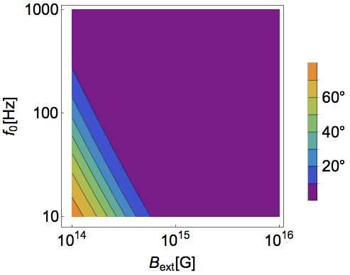
Magnetar rotation and GWs 7
Figure 5. Distribution of spin periods (colourscale) for magnetars with the shown range of Bext
and f0 at ages of 1000 yr (left) and 5000 yr (right). For all models χ0 = 1◦ and Bint = Bext .
name P/s Bext /(1014 G) An accurate value of k (or at least, its long-term average) cannot
be determined without more detailed work, so we have to rely on
1E 1547.0-5408 2.1 3.2
the qualitative arguments above. From these, we tentatively suggest
PSR J1622-4950 4.3 2.7
that existing magnetar observations indicate that f0 & 100 − 300
SGR J1745-2900 3.8 2.3
Hz and 2 . k < 3 for these stars. Furthermore, from Fig. 6, we
XTE J1810-197 5.5 2.1
see that a single measurement of χ & 15◦ from one of the more
are particularly interesting. They have in common a flat spectrum highly-magnetised (i.e. Bext ∼ 1015 G) observed magnetars would
and highly-polarised radio emission that suggests they may all have essentially rule out k ≥ 3.
a similar exterior geometry, with χ . 30◦ (Kramer et al. 2007;
Camilo et al. 2007, 2008; Levin et al. 2012; Shannon & Johnston
2013). The probability of all four radio magnetars having χ < 30◦ , 6 GRAVITATIONAL AND ELECTROMAGNETIC
assuming a random distribution of magnetic axes relative to spin RADIATION
axes, is (1 − cos 30◦ )4 ≈ 3 × 10⁻⁴ , indicating that such a distribution
6.1 GWs from newborn magnetars
is unlikely to happen by chance. Low values of χ could explain
the paucity of observed radio magnetars: if the emission is from An evolution χ → 90◦ brings a NS into an optimal geometry for
the polar-cap region, it would only be seen from a very favourable GW emission (Cutler 2002), and a few authors have previously
viewing geometry. Beyond the four radio sources, modelling of considered this scenario applied to newborn magnetars (Stella et al.
magnetar hard X-ray spectra also points to small χ (Beloborodov 2005; Dall’Osso et al. 2009), albeit without the crucial effects of the
2013; Hascoët et al. 2014), giving further weight to the idea that protomagnetar wind and self-consistent solutions for the internal
small values of χ are generic for magnetars. motions. By contrast, we have these ingredients, and hence can
Now comparing with Fig. 6, we see that – by contrast with the calculate GWs from newborn magnetars more quantitatively. In
present-day P – the present-day χ does encode interesting informa- Fig. 7 we plot the characteristic GW strain at distance d:
tion about magnetar birth. Unfortunately, as noted by Philippov et al. ! 1/2
2
(2014), the results are quite sensitive to the alignment-torque pref- 8G ǫB IΩ(t)2 sin2 χ(t) fGW
hc (t) = 4 (19)
actor k. We are also hindered by the dearth of reliable age estimates 5c d | fÛGW |
for magnetars. Nonetheless, we will still be able to draw some quite
firm conclusions, and along the way constrain the value of k. from four model magnetars with χ0 = 1◦ , averaged over sky loca-
Let us assume a fiducial mature magnetar with χ < 30◦ , tion and source orientation, following Jaranowski et al. (1998). This
Bext = 3 × 10¹⁴ G (i.e. roughly halfway between 1014 and 1015 G signal is emitted at frequency
p fGW = 2 f = Ω/π. We also show the
on a logarithmic scale) and a strong internal toroidal field (so that it design rms noise hrms = fGW Sh ( fGW ) for the detectors aLIGO
will have had χ ≈ 90◦ at early times). We first observe that such a (Abbott et al. 2018) and ET-B (Hild et al. 2008), where Sh is the
star is completely inconsistent with k = 1 unless it is far older than detector’s one-sided power spectral density. Models 1 and 2 from
5000 yr, so we regard this as a strong lower limit. Fig. 7 both have f0 = 1000 Hz and Bint = 1016 G, but the former
If k = 2, Fig. 6 shows us that the birth rotation must satisfy model has a much stronger exterior field. As a result, it is subject to
f0 & 1000 Hz if our fiducial magnetar is 1000 yr old, or f0 & 300 Hz a strong wind torque, which spins it down greatly before χ → 90◦ ,
for a 5000-yr-old magnetar. The former value may just be possible, thus reducing its GW signal compared with model 2.
in that the break-up rotation rate is typically over 1 kHz for any Next we calculate the signal-to-noise ratio (SNR) for our se-
reasonable neutron-star equation of state – but is clearly extremely lected models, following Jaranowski et al. (1998):
high. The latter value of f0 is more believable, but does require the ∫tfinal 2 Û 1/2
star to be towards the upper end of the expected magnetar age range. hc | fGW |
SNR = dt . (20)
Finally, if k = 3 the birth rotation is essentially unrestricted: hrms fGW
it implies f0 & 20 − 100 Hz for the age range 1000 − 5000 yr. As t=0
discussed earlier, however, this represents a very large enhancement Note that this expression assumes single coherent integrations. In
to the torque – with crustal motions continually regenerating the reality it will be difficult to track the evolving frequency well enough
magnetar’s corona – and sustaining this over a magnetar lifetime to perform such integrations; see discussion in Section 7.
(especially 5000 yr) therefore seems very improbable. Using aLIGO, models 1, 2, 3 and 4 have SNR =
MNRAS 000, 1–10 (0000)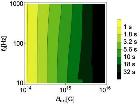
8      S. K. Lander and D. I. Jones

                  Figure 6. Distribution of χ (colourscale) for magnetars with an alignment torque prefactor of (from left to right) k = 1, 2 and
                  3; and at ages of 1000 yr (top panels) and 5000 yr (bottom panels). As before, χ0 = 1◦ and Bint = Bext for all models.

     log h                                                                           (26), however, they appear to have a different numerical prefactor
    -20
             hrms (ET)        hrms (aLIGO)                                           from ours; if this was used
                                                                                                               p in their calculations their SNR values
                                             ;                                       should be multiplied by 2/5 for direct comparison, meaning the
    -22                                                                              SNR = 5 model would become SNR ≈ 3. With our evolutions
                                                                                     we find SNR ≈ 2 for the same model. This smaller value is to be
                                                                                     expected, since we account for two pieces of physics not present
    -24                                  :    8                                      in the Dall’Osso et al. (2018) model – the magnetar wind and the
                                                                                     aligning effect of the EM torque – which are both liable to reduce
                                                                                     the GW signal.
    -26
                         7
                                                                                     6.2 Rotational-energy injection: jets and supernovae
    -28                                                           fG< [Hz]
       1                     10              100      1000                           The rapid loss of rotational energy experienced by a newborn NS
                                                                                     with very high Bext and f may be enough to power superluminous
Figure 7. GW signal hc from four model newborn magnetars, against the                supernovae, and/or GRBs. Because our wind model is based on
noise curves hrms for aLIGO and ET. Three models are for one week of signal          M11, our results for energy losses are similar to theirs, and the
at d = 20 Mpc (i.e. Virgo galaxy cluster): (1) f0 = 1 kHz, Bext = Bint = 1016
                                                                                     evolving χ only introduces order-unity differences to the overall
G, (2) f0 = 1 kHz, Bext = 0.05Bint = 5 × 10¹⁴ G, (3) f0 = 200 Hz,
Bext = 0.05Bint = 1015 G; and the final signal (4) is at d = 10 kpc (i.e. in
                                                                                     energy losses. What may change with χ, however, is which phe-
our galaxy) and has duration of one year (solid line for the first week, dotted       nomenon the lost rotational energy powers: Margalit et al. (2018)
for the rest), with Bext = 0.05Bint = 5 × 10¹³ G, f0 = 100 Hz.                       argue for a model with a partition of the energy, predominantly
                                                                                     powering a jet and GRB for χ ≈ 0◦ and thermalised emission
                                                                                     contributing to a more luminous supernova for χ ≈ 90◦ .
0.018, 0.38, 0.43, 4.0 for tfinal = 1 week. With ET, we find SNR                             The amplification of a nascent NS’s magnetic field to magnetar
values of 0.19, 4.5, 4.4, 47 for models 1, 2, 3, 4, again taking                     strengths is likely to require dynamo action, with differential rotation
tfinal = 1 week. Model 4 would be detectable for longer; taking                       playing a key role, and so we anticipate both poloidal and toroidal
instead tfinal = 1 yr gives SNR = 16 (200) for aLIGO (ET). Once χ                     components of the resulting magnetic field to be approximately
for this model reduces below 90◦ , the GW signal will gain a second                  orientated around the rotation axis. In this case, χ at birth would
harmonic at f , in addition to the one at 2 f (Jones & Andersson                     be small – and decreases further whilst the stellar matter is still
2002) . However, even after 150 yr (when the model-4 signal drops                    partially neutrino-opaque (∼ 38 s in our model). For all of this
below the ET noise curve), the star is still an almost-orthogonal ro-                phase we therefore find – following Margalit et al. (2018) – that
tator, with χ = 81◦ . In this paper, therefore, it is enough to consider             most lost rotational energy manifests itself as a GRB. Following this,
only the 2 f harmonic.                                                               the stellar matter becomes neutrino-transparent and bulk viscosity
      Recently, Dall’Osso et al. (2018) studied GWs from newborn                     activates, rapidly driving χ towards 90◦ . By this point f will have
magnetars, finding substantial SNR values even using aLIGO. To                        decreased considerably, but could still be well over 100 Hz. The
compare with them, we take one of their SNR = 5 models, which has                    star remains with χ ≈ 90◦ for ∼ 106 s in the case of an extreme
Bext /Bint = 0.019 and f0 = 830 Hz. From their equations (25) and                    millisecond magnetar, or otherwise longer; see Fig. 4. Now the

                                                                                                                                     MNRAS 000, 1–10 (0000)
Magnetar rotation and GWs                      9
rotational energy is converted almost entirely to thermal energy         us to infer the unknown Bint . A hallmark of the magnetar-birth sce-
and ceases to power the jet. Therefore, at any one point during          nario we study would be the onset of a signal with a delay of roughly
the magnetar’s evolution, one of the two EM scenarios is strongly        one minute from the initial explosion. The delay is connected with
favoured.                                                                the star becoming neutrino-transparent, and so measuring this might
                                                                         provide a probe of the newborn star’s microphysics. Note, however,
                                                                         that the actual detectability of GWs depends upon the signal anal-
6.3 Fast Radio Bursts                                                    ysis method employed – most importantly single-coherent verses
Finally, we will comment briefly on the periodicities that                multiple-incoherent integrations of the signal – and on the amount
have been seen in two repeating FRB sources (to date).                   of prior information obtained from EM observations, most impor-
The CHIME/FRB Collaboration et al. (2020) reported evidence              tantly signal start time and sky location. For a realistic search, reduc-
for a 16-day periodicity in FRB 180916.J0158+65 over a data              tions of sensitivity by a factor of 5-6 are possible (Dall’Osso et al.
set of ∼ 1 year, whilst Rajwade et al. (2020) found some-                2018; Miller et al. 2018).
what weaker evidence for a 159-day periodicity in FRB 121102                   Stronger magnetic fields do not necessarily improve prospects
from a ∼ 5-year data set. The possibility of magnetar pre-               for detecting GWs from newborn magnetars. A strong Bext causes
cession providing the required periodicity was pointed out by            a dramatic initial drop in f before orthogonalisation, resulting in a
The CHIME/FRB Collaboration et al. (2020), and developed fur-            diminished GW signal. The lost rotational energy from this phase
ther in Levin et al. (2020) and Zanazzi & Lai (2020), with the peri-     will predominantly power a GRB, and later energy losses may be
odicity being identified with the free precession period.                 seen through increased luminosity of the supernova. Less electro-
      As noted by Zanazzi & Lai (2020), the lack of a measurement        magnetically spectacular supernovae may therefore be better targets
of a spin period introduces a significant degeneracy (between P and       for GW searches.
ǫB , in our notation). Nevertheless, a few common-sense considera-             The birth of a NS in our galaxy2 need not have such extreme
tions help to further constrain the model. In addition to reproducing    parameters to produce interesting levels of GW emission, as long
the free precession period, a successful model also has to predict no    as it has a fairly strong internal toroidal field, Bint & 1014 G, and
significant evolution in spin frequency (as noted by Zanazzi & Lai         f0 & 100 Hz. These are plausible birth parameters for a typical radio
(2020)) or in χ, over the ∼ 1–5 year durations of the observations.      pulsar, since Bext will typically be somewhat weaker than Bint . Such
Also, the precession angle cannot be too close to zero or π/2, as        a star will initially experience a similar evolution to that reported
otherwise there would be no geometric modulation of the emission.        here, but slower, giving the star time to cool and begin forming
Finally, a requirement specific to the model of Levin et al. (2020) is    a crust. Afterwards, the evolution of χ will probably proceed in
that the magnetar should be only tens of years old.                      a slow, stochastic way dictated primarily by crustal-failure events:
      Our simulations show that requiring χ to take an intermedi-        crustquakes or episodic plastic flow. Regardless of the details of this
ate value is a significant constraint. At sufficiently late times the       evolutionary phase, we find that the long-timescale trend for all NSs
electromagnetic torque wins out, and the star aligns ( χ → 0), an        should be the alignment of their rotation and magnetic axes, which
effect not considered in either Levin et al. (2020) or Zanazzi & Lai      is in accordance with observations (Tauris & Manchester 1998;
(2020). We clearly can accommodate stars of ages ∼ 10 − 100 yr           Weltevrede & Johnston 2008; Johnston & Karastergiou 2019).
with such intermediate χ values; see the top panel of Fig. 4. Such             Many of our conclusions will not be valid for NSs whose mag-
magnetars in this age range experience, however, considerable spin-      netic fields are dominantly poloidal, rather than toroidal. In this
down: from our evolutions we find a decrease of around 4% in the          case the magnetically-induced distortion is oblate, and there is no
spin and precession frequencies over a year at age 10 yr, and a 0.5%     obvious mechanism for χ to increase; it will simply decrease from
annual decrease at age 100 yr. More work is clearly needed to see        birth. The expectation that all NSs eventually tend towards χ ≈ 0◦
whether this is compatible with the young-magnetar model, and we         remains true, but our constraints on magnetar birth would likely
intend to pursue this matter in a separate study.                        become far weaker and the GW emission from this phase negligi-
                                                                         ble. The lost rotational energy from the newborn magnetar would
                                                                         power a long-duration GRB almost exclusively, at the expense of
                                                                         any luminosity enhancement to the supernova. Poloidal-dominated
7 DISCUSSION                                                             fields are, however, problematic for other reasons: it is not clear how
Inclination angles encode important information about NSs that           they would be generated, whether they would be stable, or whether
cannot be otherwise constrained. In particular, hints that observed      magnetar activity could be powered in the absence of a toroidal field
magnetars generically have small χ places a significant and inter-        stronger than the inferred exterior field. This aspect of the life of
esting constraint on their rotation rates at birth, f0 & 100 − 300       newborn magnetars clearly deserves more detailed modelling.
Hz, and shows that their exterior torque must be stronger than that
predicted for pulsar magnetospheres. More detailed modelling of
this magnetar torque may increase this minimum f0 . Because our          ACKNOWLEDGEMENTS
models place lower limits on f0 (from the shape of the contours
                                                                         We thank Simon Johnston and Patrick Weltevrede for valuable dis-
of Fig. 6), they complement other work indicating upper limits of
                                                                         cussions about inclination angles. We are also grateful to Cris-
 f0 . 200 Hz, based on estimates of the explosion energy from
                                                                         tiano Palomba, Wynn Ho, and the referees for their construc-
magnetar-associated supernovae remnants (Vink & Kuiper 2006).
                                                                         tive criticism. SKL acknowledges support from the European
     Typically, a newborn magnetar experiences an evolution where
                                                                         Union’s Horizon 2020 research and innovation programme under
χ → 90◦ within one minute. At this point it emits its strongest GW
signal. For rapidly-rotating magnetars born in the Virgo cluster, for
which the expected birth rate is & 1 per year (Stella et al. 2005),      2 It is optimistic – but not unreasonable – to anticipate seeing such an
there are some prospects for detection of this signal with ET, pro-      event, with birth rates of maybe a few per century (Lorimer et al. 2006;
vided that the ratio Bext /Bint is small. Such a detection would allow   Faucher-Giguère & Kaspi 2006).

MNRAS 000, 1–10 (0000)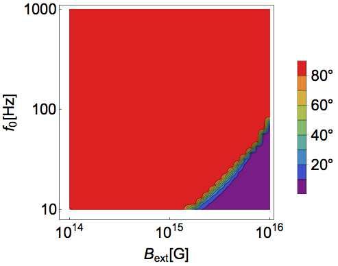
10       S. K. Lander and D. I. Jones
the Marie Skłodowska-Curie grant agreement No. 665778, via fel-                 Qian Y. Z., Woosley S. E., 1996, ApJ, 471, 331
lowship UMO-2016/21/P/ST9/03689 of the National Science Cen-                    Rajwade K. M., et al., 2020, arXiv e-prints, p. arXiv:2003.03596
tre, Poland. DIJ acknowledges support from the STFC via grant                   Reisenegger A., Goldreich P., 1992, ApJ, 395, 240
numbers ST/M000931/1 and ST/R00045X/1. Both authors thank                       Rembiasz T., Guilet J., Obergaulinger M., Cerdá-Durán P., Aloy M. A.,
the PHAROS COST Action (CA16214) for partial support.                                Müller E., 2016, MNRAS, 460, 3316
                                                                                Ruderman M., Zhu T., Chen K., 1998, ApJ, 492, 267
                                                                                Şaşmaz Muş S., Çıkıntoğlu S., Aygün U., Ceyhun Andaç I., Eks, i K. Y.,
                                                                                     2019, arXiv e-prints, p. arXiv:1904.06769
                                                                                Schatzman E., 1962, Annales d’Astrophysique, 25, 18
REFERENCES
                                                                                Shannon R. M., Johnston S., 2013, MNRAS, 435, L29
Abbott B. P., et al., 2018, Living Reviews in Relativity, 21, 3                 Spitkovsky A., 2006, ApJ, 648, L51
Beloborodov A. M., 2013, ApJ, 762, 13                                           Spitzer Jr. L., 1958, in Lehnert B., ed., IAU Symposium Vol. 6, Electromag-
Beloborodov A. M., Thompson C., 2007, ApJ, 657, 967                                  netic Phenomena in Cosmical Physics. p. 169
Bucciantini N., Thompson T. A., Arons J., Quataert E., Del Zanna L., 2006,      Stella L., Dall’Osso S., Israel G. L., Vecchio A., 2005, ApJ, 634, L165
    MNRAS, 368, 1717                                                            Tauris T. M., Manchester R. N., 1998, MNRAS, 298, 625
Camilo F., Reynolds J., Johnston S., Halpern J. P., Ransom S. M., van Straten   Tayler R. J., 1980, MNRAS, 191, 151
    W., 2007, ApJ, 659, L37                                                     Tendulkar S. P., Cameron P. B., Kulkarni S. R., 2012, ApJ, 761, 76
Camilo F., Reynolds J., Johnston S., Halpern J. P., Ransom S. M., 2008,         The CHIME/FRB Collaboration et al., 2020, arXiv e-prints,
    ApJ, 679, 681                                                                    p. arXiv:2001.10275
Chandrasekhar S., Fermi E., 1953, ApJ, 118, 116                                 Thompson C., Duncan R. C., 1993, ApJ, 408, 194
Contopoulos I., Kazanas D., Fendt C., 1999, ApJ, 511, 351                       Thompson C., Duncan R. C., 1995, MNRAS, 275, 255
Cutler C., 2002, Phys. Rev. D, 66, 084025                                       Thompson C., Lyutikov M., Kulkarni S. R., 2002, ApJ, 574, 332
Cutler C., Jones D. I., 2001, Phys. Rev. D, 63, 024002                          Thompson T. A., Chang P., Quataert E., 2004, ApJ, 611, 380
Dall’Osso S., Shore S. N., Stella L., 2009, MNRAS, 398, 1869                    Timokhin A. N., 2006, MNRAS, 368, 1055
Dall’Osso S., Stella L., Palomba C., 2018, MNRAS, 480, 1353                     Vink J., Kuiper L., 2006, MNRAS, 370, L14
Deutsch A. J., 1955, Annales d’Astrophysique, 18, 1                             Weltevrede P., Johnston S., 2008, MNRAS, 387, 1755
Faucher-Giguère C.-A., Kaspi V. M., 2006, ApJ, 643, 332                         Woosley S. E., 2010, ApJ, 719, L204
Ghosh P., Lamb F. K., 1978, ApJ, 223, L83                                       Younes G., Baring M. G., Kouveliotou C., Harding A., Donovan S., Göğüs,
Giacomazzo B., Perna R., 2013, ApJ, 771, L26                                         E., Kaspi V., Granot J., 2017, ApJ, 851, 17
Goldreich P., Julian W. H., 1969, ApJ, 157, 869                                 Zanazzi J. J., Lai D., 2020, ApJ, 892, L15
Guilet J., Müller E., Janka H.-T., 2015, MNRAS, 447, 3992
Hascoët R., Beloborodov A. M., den Hartog P. R., 2014, ApJ, 786, L1
Hild S., Chelkowski S., Freise A., 2008, arXiv e-prints, p. arXiv:0810.0604
Jaranowski P., Królak A., Schutz B. F., 1998, Phys. Rev. D, 58, 063001
Johnston S., Karastergiou A., 2019, MNRAS, 485, 640
Jones P. B., 1976, Ap&SS, 45, 369
Jones D. I., Andersson N., 2002, MNRAS, 331, 203
Kasen D., Bildsten L., 2010, ApJ, 717, 245
Kashiyama K., Murase K., Bartos I., Kiuchi K., Margutti R., 2016, ApJ,
    818, 94
Kramer M., Stappers B. W., Jessner A., Lyne A. G., Jordan C. A., 2007,
    MNRAS, 377, 107
Lai D., 2001, in Astrophysical Sources for Ground-Based Gravitational Wave
    Detectors.
Lander S. K., 2016, ApJ, 824, L21
Lander S. K., Jones D. I., 2009, MNRAS, 395, 2162
Lander S. K., Jones D. I., 2017, MNRAS, 467, 4343
Lander S. K., Jones D. I., 2018, MNRAS, 481, 4169
Lasky P. D., Glampedakis K., 2016, MNRAS, 458, 1660
Levin L., et al., 2012, MNRAS, 422, 2489
Levin Y., Beloborodov A. M., Bransgrove A., 2020, arXiv e-prints,
    p. arXiv:2002.04595
Lorimer D. R., et al., 2006, MNRAS, 372, 777
Margalit B., Metzger B. D., Thompson T. A., Nicholl M., Sukhbold T., 2018,
    MNRAS, 475, 2659
Mestel L., 1968a, MNRAS, 138, 359
Mestel L., 1968b, MNRAS, 140, 177
Mestel L., Spruit H. C., 1987, MNRAS, 226, 57
Mestel L., Takhar H. S., 1972, MNRAS, 156, 419
Metzger B. D., Thompson T. A., Quataert E., 2007, ApJ, 659, 561
Metzger B. D., Giannios D., Thompson T. A., Bucciantini N., Quataert E.,
    2011, MNRAS, 413, 2031
Miller A., et al., 2018, Phys. Rev. D, 98, 102004
Olausen S. A., Kaspi V. M., 2014, ApJS, 212, 6
Page D., Geppert U., Weber F., 2006, Nuclear Physics A, 777, 497
Philippov A., Tchekhovskoy A., Li J. G., 2014, MNRAS, 441, 1879
Pons J. A., Reddy S., Prakash M., Lattimer J. M., Miralles J. A., 1999, ApJ,
    513, 780

                                                                                                                                MNRAS 000, 1–10 (0000)
You can also read