Peaberry and normal coffee bean classification using CNN, SVM, and KNN: Their implementation in and the limitations of Raspberry Pi 3
←
→
Page content transcription
If your browser does not render page correctly, please read the page content below
AIMS Agriculture and Food, 7(1): 149–167.
                                                           DOI: 10.3934/agrfood.2022010
                                                           Received: 28 September 2021
                                                           Revised: 14 February 2022
                                                           Accepted: 21 March 2022
                                                           Published: 25 March 2022
http://www.aimspress.com/journal/agriculture

Research article

Peaberry and normal coffee bean classification using CNN, SVM, and
KNN: Their implementation in and the limitations of Raspberry Pi 3

Hira Lal Gope1,2,* and Hidekazu Fukai1

1
    Faculty of Engineering, Gifu University, 501-1193, Japan
2
    Faculty of Agricultural Engineering and Technology, Sylhet Agricultural University, Sylhet-3100,
    Bangladesh

* Correspondence: Email: hlgope@sau.ac.bd; Tel: +819029335826.

Abstract: Peaberries are a special type of coffee bean with an oval shape. Peaberries are not
considered defective, but separating peaberries is important to make the shapes of the remaining
beans uniform for roasting evenly. The separation of peaberries and normal coffee beans increases
the value of both peaberries and normal coffee beans in the market. However, it is difficult to sort
peaberries from normal beans using existing commercial sorting machines because of their
similarities. In previous studies, we have shown the availability of image processing and machine
learning techniques, such as convolutional neural networks (CNNs), support vector machines (SVMs),
and k-nearest-neighbors (KNNs), for the classification of peaberries and normal beans using a
powerful desktop PC. As the next step, assuming the use of our system in the least developed
countries, this study was performed to examine their implementation in and the limitations of
Raspberry Pi 3. To improve the performance, we modified the CNN architecture from our previous
studies. As a result, we found that the CNN model outperformed both linear SVM and KNN on the
use of Raspberry Pi 3. For instance, the trained CNN could classify approximately 13.77 coffee bean
images per second with 98.19% accuracy of the classification with 64×64 pixel color images on
Raspberry Pi 3. There were limitations of Raspberry Pi 3 for linear SVM and KNN on the use of
large image sizes because of the system’s small RAM size. Generally, the linear SVM and KNN
were faster than the CNN with small image sizes, but we could not obtain better results with both the
linear SVM and KNN than the CNN in terms of the classification accuracy. Our results suggest that
the combination of the CNN and Raspberry Pi 3 holds the promise of inexpensive peaberries and a
normal bean sorting system for the least developed countries.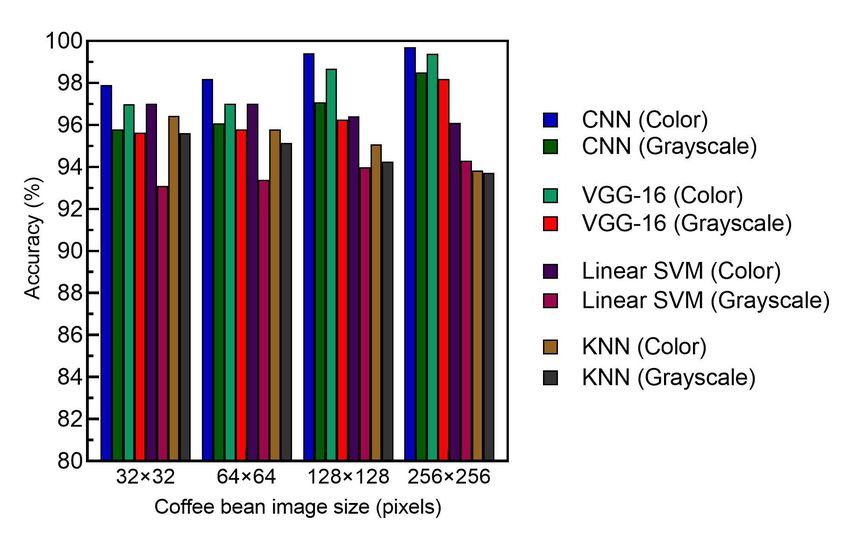
150

Keywords: Convolutional Neural Networks (CNN); coffee bean; K-Nearest-Neighbors (KNN);
peaberry; Raspberry Pi 3; Support Vector Machine (SVM)

1.   Introduction

      Coffee beans comprise one of the world’s most extensively traded agricultural products [1,2].
Brazil, Vietnam, Colombia, and Indonesia earn a large number of foreign currencies, which is vital to
their population’s livelihood [3,4].
      The visible features of peaberries include a diameter smaller than a normal, flat-sided pair of
coffee beans, which resemble a football, as they appear to be thicker and more rounded [5]. There are
two embryos in a normal coffee cherry, both of which are fertilized and grow inside a confined space,
resulting in the typical hemispherical shape of coffee beans. Peaberries occur when only a single
embryo is fertilized inside the coffee cherry [6]. Peaberries are limited; approximately 7% of any green
coffee crop consists of peaberries [3,7]. Peaberries are not specific to any particular area, and they can
grow anywhere [8].
      It is important to separate peaberries from normal beans for the following reasons: First,
peaberries are often separated to ensure an even roast in high-grade coffee. Because the roasting
process significantly affects the taste of coffee and the control of the roasting time depending on
bean size is essential, the uniformity of coffee bean size is vital. Even if the beans are sorted by size,
separating peaberries is preferred, especially for high-grade coffee, because their shape differs from
that of normal beans [9]. Another reason for distinguishing peaberries from normal beans is that the
price of a collection of peaberries increases significantly compared to normal beans due to their
rarity [7].
      Several types of automatic coffee bean sorting machines are already in use in developed
countries. The main functions of the sorting machines are to sort the beans by size and/or remove
defective beans, such as black, sour, and broken beans, from the normal beans. The machines sort the
defects mainly by using color as a clue, so the sorting of peaberries is a hard task for conventional
sorting machines because the color of peaberries is similar to the color of normal beans. To the best
of our knowledge, there are no automatic sorting machines that can sort peaberries.
      Deep learning models have been ubiquitously utilized for image processing. The importance of
classification with quality can be noticed in the number of research publications that work with not
only neural networks but also simple image processing and other machine learning techniques to sort
various vegetables, fruits, crops, beans, etc. The authors used deep learning architecture in the area of
tomato crops and found an accuracy of 97.29% and 97.49%, respectively [10]. In another study, the
authors used a simple image processing technique in the field of carrot fruit. The classification
accuracies of the linear discriminant analysis (LDA) and quadratic discriminant analysis (QDA)
methods were 92.59% and 96.30%, respectively [11]. The authors applied machine-learning methods
such as C4.5 decision tree, logistic regression (LR), support vector machine (SVM), and multilayer
perceptron (MLP) for classifying nine major summer crops. The MLP and SVM methods obtained a
better accuracy of 88% than LR (86%) and C4.5 (79%) [12]. However, only a few studies have
employed deep learning for coffee bean classification. We have been investigating the application of
machine learning techniques, including deep learning models, to coffee bean classification. We
applied a deep CNN to classify green coffee beans into several defective groups, including

AIMS Agriculture and Food                                                        Volume 7, Issue 1, 149–167.
151

peaberries as a class, with accuracies ranging from 72.41% to 98.75% [13]. One limitation of this
study was that the number of peaberries used for training was insufficient, resulting in lower
accuracy for peaberries. In another study, we examined the availability of Raspberry Pi 3 and a deep
CNN method for the classification of several types of defective coffee beans [9]. In our previous
study [14], we focused on the sorting of peaberries and normal beans using the CNN on a desktop
PC, resulting in accuracies ranging from 97.26% to 98.53% for four different image sizes.
     As the next step, this study was performed to examine the implementation of three major
machine learning algorithms, e.g., convolutional neural networks (CNNs), support vector
machines (SVMs), and k-nearest-neighbors (KNNs), on the Raspberry Pi 3 to classify peaberries and
normal beans, assuming the use of our system in the least developed countries. We compared the
performances and examined their limitations. In each algorithm, we estimated the calculation time
and the accuracy of the classification to verify the availability of Raspberry Pi 3 for classification in
practical use.
     In the next section, we will describe the materials of peaberries and normal green coffee beans,
the experimental setup, and each machine learning method. In Section 3, we describe both the
experimental results and the discussion, following the conclusion in Section 4.

2.   Materials and methods

2.1. Green coffee beans

     The collected coffee bean type was Arabica. Dry green coffee bean samples were collected from
farmers in Timor-Leste. In this study, two types of green coffee beans are described below:
     Peaberry: Peaberries are a single embryo that is fertilized inside coffee cherries instead of the
usual flat-sided pair of coffee beans. Peaberries are oval-shaped beans. They are also known as
‘caracol’, ‘perla’, and ‘perle’ [15]. Peaberries tend to be surprisingly acidic with a more intense
flavor than normal beans. Peaberries are often hand-selected by farmers from the total harvest and
sold as a special grade rather than as normal beans (Figure 1(a)) [3,16].
     Normal (no defect): A normal coffee cherry will contain two beans with facing flat sides that are
similar to peanut halves (Figure 1(b)) [3,7]. These beans are sometimes referred to as ‘flat beans’.
They are perfect and not defective.

                            Figure 1. Coffee beans: (a) peaberry and (b) normal.

AIMS Agriculture and Food                                                          Volume 7, Issue 1, 149–167.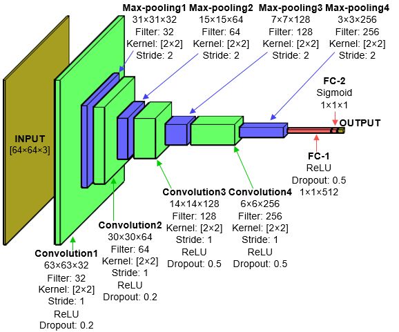
152

2.2. Image acquisition

     Peaberries and normal green coffee bean samples were collected from farmers in Timor-Leste.
Coffee beans were placed on size A4 white paper, and images were collected with a Nikon digital
camera (D5100, Nikon, Tokyo, Japan). The camera parameters were set up as follows: F/16
f-number, exposure time of 1/60 s, ISO 200, exposure compensation of 1.3, autofocus mode, image
resolution of 4928 x 3264, and a position of one meter (1 m) above the surface of the beans. Three
general lighting devices were employed for the photographic environment, as shown in Figure 2.
Both the front-side and back-side of the coffee beans were taken. Then, image sizes were resized to
32 × 32, 64 × 64, 128 × 128, and 256 × 256 pixels, and we also prepared a set of grayscale images
with the same size. As the image preprocessing, we applied resizing and grayscale conversion using
OpenCV, Open Source Computer Vision Library.
     Although the input of CNN, SVM, and KNN can be the features of images extracted by
preliminary image processing, we used raw pixel values of images as the input of each CNN, SVM,
and KNN in this work. We can expect the network layers of the CNN will extract the features, such
as shape, colors, and textures automatically. Also, SVM and KNN accept raw pixel values of images
as input for classification.
     The objective to prepare several sizes of images for each color and grayscale was to examine
the best size of images for the Raspberry Pi 3. The larger image size has more pixel information than
a smaller image (Figure 3(a), (b)), and makes the accuracy of the classification higher, whereas the
smaller image size makes the processing speed faster.
     The images were manually labeled as peaberries and normal coffee beans. All images of the
coffee beans were divided into three groups: training data, validation data, and test data. In the neural
network training phase, the validation data were utilized to confirm the transition of the classification
accuracy. The test data were applied to measure the accuracy (Section 2.7) of the neural networks’
sorting ability. Table 1 represents the total number of images for each group.

                                 Figure 2. Photographic environment.

AIMS Agriculture and Food                                                       Volume 7, Issue 1, 149–167.
153
Figure 3. Sample images of coffee bean: (a) peaberry and (b) normal bean in color (left
side) and grayscale (right side).
Table 1. Number of images for each task.
Task Training Validation Test Total
Peaberry (color) 1144 143 143 1430
Peaberry (grayscale) 1144 143 143 1430
Normal (color) 1520 190 190 1900
Normal (grayscale) 1520 190 190 1900
2.3. Convolutional neural networks
Convolutional neural networks (CNNs) are a form of an artificial neural network; these techniques
have dramatically improved the performance of image recognition, object detection, speech
recognition, natural language processing, drug discovery and genomics, and many other domains [17–19].
The basic CNN architecture consists of three types of layers: convolutional, pooling, and fully
connected layers.
AIMS Agriculture and Food Volume 7, Issue 1, 149–167.154
Figure 4. Proposed structure of the CNN model for a 64 × 64 color image: four
convolutional layers, four max-pooling layers, and two fully connected layers.
Table 2 describes the specifications of the CNN model in this study for 32 × 32, 64 × 64,
128 × 128, and 256 × 256 input image sizes. The structure of the model for 64×64 is described in
Figure 4. All the models were written by using Python libraries, such as Keras, TensorFlow, and
Numpy. All the proposed CNN models consist of four convolutional layers, and each is followed by a
max-pooling layer. The first convolutional layer uses 32 filters and is followed by 64, 128, and 256
filters. Each convolutional layer has a 2 × 2 receptive field that is applied with a stride of 1 pixel. Each
max-pooling layer has 2 × 2 regions at a stride of 2 pixels. The Rectified Linear Unit (ReLU)
activation function is applied consecutively to each convolutional layer. The last convolutional
layer is followed by two fully connected (FC) hidden layers. The two FC layers (FC-1 and FC-2)
are employed to increase the performance of the neural network [20,21]. We applied dropout (0.2,
0.2, 0.5, 0.5, and 0.5) in the four convolutional layers and the FC-1 layer to prevent overfitting in the
network [22].
The proposed CNN model was tuned with different batch sizes (8, 16, 32), epochs (50, 60, 100),
optimizer (SGD, Adam), activation function (‘relu’ and ‘tanh’), and learning rate (0.01, 0.001). We
found the best performance for the following conditions: 32 batch size, 100 epochs, SGD (Stochastic
Gradient Descent) optimizer, relu activation function, and 0.01 learning rate. The sigmoid function
AIMS Agriculture and Food Volume 7, Issue 1, 149–167.155
yields a value between 0 and 1, and the output is generally interpreted as a probability on neural
networks. After the calculation of the probability of peaberry class using the sigmoid function, we
classified the input image of a bean as the peaberry if the probability is more than 0.5 as a threshold
value.
Table 2. Parameters of CNN for four kinds of image datasets.
(a) 32 × 32 image size
Layer name Filter shape Stride (s) Output map shape Activation
(H × H × K) (W × W × M) function f(∙)
Input - - 32 × 32 × 3 -
Convolution1 2 ×2 ×3 1 31 × 31 × 32 ReLU
Max-Pooling1 2 × 2 × 32 2 15 × 15 × 32 -
Dropout (0.2) - - 15 × 15 × 32 -
Convolution2 2 × 2 × 32 1 14 × 14 × 64 ReLU
Max-Pooling2 2 × 2 × 64 2 7 × 7 × 64 -
Dropout (0.2) - - 7 × 7 × 64 -
Convolution3 2 × 2 × 64 1 6 × 6 × 128 ReLU
Max-Pooling3 2 × 2 × 128 2 3 × 3 × 128 -
Dropout (0.5) - - 3 × 3 × 128 -
Convolution4 2 × 2 × 128 1 2 × 2 × 256 ReLU
Max-Pooling4 2 × 2 × 256 2 1 × 1 × 256 -
Dropout (0.5) - - 1 × 1 × 256 -
FullConnected1 - - 1 × 1 × 512 ReLU
Dropout (0.5) - - 1 × 1 × 512 -
FullConnected2 - - 1 ×1 ×1 Sigmoid
(b) 64 × 64 image size
Input - - 64 × 64 × 3 -
Convolution1 2 ×2 ×3 1 63 × 63 × 32 ReLU
Max-Pooling1 2 × 2 × 32 2 31 × 31 × 32 -
Dropout (0.2) - - 31 × 31 × 32 -
Convolution2 2 × 2 × 32 1 30 × 30 × 64 ReLU
Max-Pooling2 2 × 2 × 64 2 15 × 15 × 64 -
Dropout (0.2) - - 15 × 15 × 64 -
Convolution3 2 × 2 × 64 1 14 × 14 × 128 ReLU
Max-Pooling3 2 × 2 × 128 2 7 × 7 × 128 -
Dropout (0.5) - - 7 × 7 × 128 -
Convolution4 2 × 2 × 128 1 6 × 6 × 256 ReLU
Max-Pooling4 2 × 2 × 256 2 3 × 3 × 256 -
Dropout (0.5) - - 3 × 3 × 256 -
FullConnected1 - - 1 × 1 × 512 ReLU
Dropout (0.5) - - 1 × 1 × 512 -
FullConnected2 - - 1 ×1 ×1 Sigmoid
Continued on the next page
AIMS Agriculture and Food Volume 7, Issue 1, 149–167.156
(c) 128 × 128 image size
Layer name Filter shape Stride (s) Output map shape Activation
(H × H × K) (W × W × M) function f(∙)
Input - - 128 × 128 × 3 -
Convolution1 2 ×2 ×3 1 127 × 127 × 32 ReLU
Max-Pooling1 2 × 2 × 32 2 63 × 63 × 32 -
Dropout (0.2) - - 63 × 63 × 32 -
Convolution2 2 × 2 × 32 1 62 × 62 × 64 ReLU
Max-Pooling2 2 × 2 × 64 2 31 × 31 × 64 -
Dropout (0.2) - - 31 × 31 × 64 -
Convolution3 2 × 2 × 64 1 30 × 30 × 128 ReLU
Max-Pooling3 2 × 2 × 128 2 15 × 15 × 128 -
Dropout (0.5) - - 15 × 15 × 128 -
Convolution4 2 × 2 × 128 1 14 × 14 × 256 ReLU
Max-Pooling4 2 × 2 × 256 2 7 × 7 × 256 -
Dropout (0.5) - - 7 × 7 × 256 -
FullConnected1 - - 1 × 1 × 512 ReLU
Dropout (0.5) - - 1 × 1 × 512 -
FullConnected2 - - 1 ×1 ×1 Sigmoid
(d) 256×256 image size
Input - - 256 × 256 × 3 -
Convolution1 2 ×2 ×3 1 255 × 255 × 32 ReLU
Max-Pooling1 2 × 2 × 32 2 127 × 127 × 32 -
Dropout (0.2) - - 127 × 127 × 32 -
Convolution2 2 × 2 × 32 1 126 × 126 × 64 ReLU
Max-Pooling2 2 × 2 × 64 2 63 × 63 × 64 -
Dropout (0.2) - - 63 × 63 × 64 -
Convolution3 2 × 2 × 64 1 62 × 62 × 128 ReLU
Max-Pooling3 2 × 2 × 128 2 31 × 31 × 128 -
Dropout (0.5) - - 31 × 31 × 128 -
Convolution4 2 × 2 × 128 1 30 × 30 × 256 ReLU
Max-Pooling4 2 × 2 × 256 2 15 × 15 × 256 -
Dropout (0.5) - - 15 × 15 × 256 -
FullConnected1 - - 1 × 1 × 512 ReLU
Dropout (0.5) - - 1 × 1 × 512 -
FullConnected2 - - 1 ×1 ×1 Sigmoid
2.4. Visual Geometry Group (VGG-16)
The VGG-16 is a very simple, straightforward architecture. The number 16 in the name VGG
refers to the fact that it is 16 layers deep neural network. Each VGG block consists of a sequence of
convolutional layers, which are followed by a max-pooling layer. VGG-16 is composed of 13
convolutional layers, 5 max-pooling layers, and 3 fully connected layers. The same kernel size (3 × 3)
is applied over all convolutional layers with a stride of 1 pixel. Each max-pooling layer has 2 × 2
AIMS Agriculture and Food Volume 7, Issue 1, 149–167.157
regions. The VGG model has two fully connected hidden layers and one fully connected output
layer [23]. The Rectified Linear Unit (ReLU) activation function is assigned consecutively to each
convolutional layer. The last convolutional layer is followed by fully connected (FC) hidden layers.
2.5. Support vector machine
A support vector machine (SVM) is a learning technique that is initially designed to fit a linear
boundary between two binary problem samples, ensuring maximum robustness in terms of isotropic
uncertainty tolerance. Various types of functions, such as linear, polynomial, and radial basis
function (RBFs), are widely applied to transform the input space into the desired function [24,25]. In
this study, we used a linear SVM; the training set of features was applied as the input to train a
conventional linear SVM, and the testing set of features was applied to obtain image labels for frame
test prediction. The scikit-learn machine learning library was chosen for implementing the linear
SVM. We examined the SVM method with the different parameters of gamma (‘0.1’, ‘auto’), C = 1,
and kernel (‘linear’, ‘rbf’), and we found the best accuracy for gamma = 0.1, C = 1, and kernel =
linear.
2.6. K-nearest-neighbors
The k-nearest-neighbors (KNN) method is one of the most important data mining techniques
that attempts to classify an unknown sample based on the known classification of its neighbors [26].
The KNN algorithm simply stores the image dataset during the training process, and when it obtains
a new image, it classifies this image into a category that is very similar to the new image. In this
study, classification using the KNN method was carried out with a 5-times-trial using different k
values for each experiment. We partitioned the data into 10 folds and utilized 10-1 folds for training
and the remainder (1-fold) for validation. The k values of 1, 3, 5, 7, and 9 were applied to obtain the
best performance for peaberries and normal coffee bean images [27].
2.7. Classification accuracy
The classification accuracy for the CNN, linear SVM and KNN methods refers to the ratio of
items that are positive and classified as positive and to those that are negative and classified as negative,
as described in equation (1).
(1)
where TP, TN, FP, and FN are the number of true positives, true negatives, false positives, and false
negatives, respectively.
2.8. Raspberry Pi and Camera Module
This research demonstrates a real-time application for coffee bean image classification by using
a Raspberry Pi [28]. The Raspberry Pi Foundation developed a series of credit-card-sized single,
electronic board, compute modules named Raspberry Pi to promote the teaching of basic computer
science in institutes and developed countries [29]. In this study, we chose the Raspberry Pi 3 Model
AIMS Agriculture and Food Volume 7, Issue 1, 149–167.158
B. The Raspberry Pi 3 has 1 GB of RAM, a 64-bit ARM quad-core processor, 4 USB ports, a wired
LAN port, and one HDMI port and supports Wi-Fi and Bluetooth wireless connections. Various
additional modules, such as a camera, display, a micro SD port for loading the operating system and
storing data, and different sensors, can be directly connected to the base. Raspberry Pi 3 also has a
GPU and can be controlled by a simple LCD. In addition, the model also has an input/output
terminal (GPIO) with 40 general-purpose pins. The GPIO allows us to use electronic devices and
handle various sensors.
The original Raspberry Pi 3 Camera Module V2 was used for the camera module and was
connected to the CSI-2 connector. The Camera Module V2 has an 8-megapixel SONY IMX219
sensor and can be used to capture high-definition video and still photography. Here, the libraries
bundled with the camera can be used. The system supports 1080p30, 720p60, and VGA90 video
modes and still captures [30]. The camera module was attached via a 15 cm ribbon cable to the CSI
port on the Raspberry Pi 3. In this research, the original camera module was used instead of USB
third-party cameras. The CSI-2 connector is faster than USB 2.0 [9].
The Raspberry Pi is suitable for our project because the module can be available worldwide at a
very cheap price. The Raspberry Pi 3 Model B is the third generation Raspberry Pi. The total cost of
the Raspberry Pi 3 system was estimated at $50.
3. Results and discussion
In this experiment, the front-side and back-side coffee bean images for both normal and
peaberry were taken separately. We used both front-side and back-side images of a bean in the
training set, validation set, and test set by mixing the order of them. For instance, the front-side of
beans were used in the training set, as well as the back-side of the same beans, which were also used
in the training set. It means that the system classifies classes are only ‘normal beans’ and ‘peaberries’
regardless of front-side or back-side, assuming the practical use. This experiment was a preliminary
experiment for the whole system we will develop. On the whole system, a large quantity of
arranged/not-arranged beans flows on a board, like a conveyor belt, regardless of the front-side or
back-side. The system must classify the ‘normal’ and ‘peaberry’ regardless of the sides. In this work,
we evaluated the performance and examined the limitations of three major machine learning
algorithms, e.g., convolutional neural networks (CNN), support vector machines (SVM), and
k-nearest-neighbors (KNN), for four different image sizes, e.g., 32×32, 64×64, 128×128, and
256×256 pixels. We also examined the differences between color image datasets and grayscale
image datasets. First, we trained each model with all the above mentioned parameter combinations
and evaluated the classification accuracies on the desktop PC (Section 3.2). Second, we examined
the calculation time and limitations of Raspberry Pi 3 using the same datasets and models that were
trained on desktop PC (Section 3.3). If we use the same datasets and pretrained models for
classification, we just obtain the same results regardless of the calculation platforms. The differences
between the desktop PC and Raspberry Pi 3 are the calculation time and limitations depending on
CPU power, memory size, and etc. Before the comparison among the CNN, linear SVM, and KNN,
we experimented with different k values (k = {1, 3, 5, 7, 9}) of the KNN method to obtain a better k
value (Section 3.1).
AIMS Agriculture and Food Volume 7, Issue 1, 149–167.159
3.1. Selection of k value for KNN method
The purpose of this part of the experiment is to ensure the classification efficiency of the KNN
classification method and to improve the accuracy of the classification method. The results of the
classification accuracy for different k values and image sizes are summarized in Table 3 and Figure 5.
For both the color image case and grayscale image case and for any k value cases, we obtained the best
classification accuracy with the smallest image size of 32×32 pixels, and the accuracy decreased as the
image size increased. Generally, a larger image size has more information to be used in the
classification. On the other hand, it is known that the KNN method tends to fail classifications as the
image size increases because the method uses the Euclidean distance to estimate the nearness and the
‘curse of dimensionality’ problem arises at larger image sizes [31]. Regarding the k value, we obtained
the best accuracy with k = 5 in most cases, so we use k = 5 hereafter in the KNN method.
Table 3. Results of average accuracy (mean) and standard deviation (SD) for different k
values on the desktop PC.
(a) Color image
32 × 32 64 × 64 128 × 128 256 × 256
Value of k Mean SD Mean SD Mean SD Mean SD
k=1 95.80 0.015572 95.08 0.012438 94.29 0.013430 93.30 0.016019
k=3 96.40 0.011674 95.95 0.007524 94.86 0.011187 93.63 0.014423
k=5 96.43 0.012215 95.80 0.013430 95.08 0.014725 93.84 0.018525
k=7 95.89 0.014089 95.74 0.012079 95.11 0.015118 94.05 0.014834
k=9 95.86 0.017326 95.41 0.012901 95.02 0.013957 93.90 0.017167
(b) Grayscale image
k=1 95.14 0.013564 94.53 0.013564 93.90 0.015678 92.98 0.027361
k=3 95.59 0.011061 94.92 0.009544 94.20 0.010503 93.57 0.021123
k=5 95.62 0.015325 95.14 0.013710 94.26 0.017014 93.73 0.025807
k=7 95.32 0.016582 94.89 0.013430 94.41 0.016702 93.88 0.023100
k=9 95.23 0.021303 94.74 0.014385 94.26 0.017364 93.74 0.024791
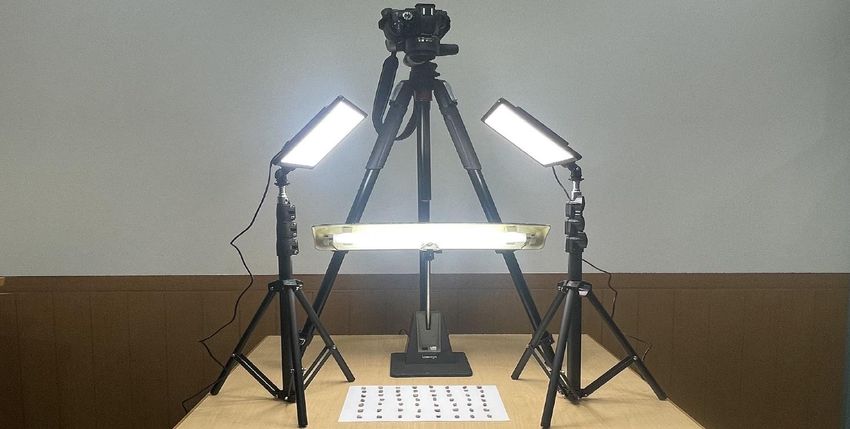
3.2. Performance of the classification on desktop PC
We compared the performance of the three machine learning methods for four different image
sizes in terms of the classification accuracy on the desktop PC ((Table 4 (a), (b)) and Figure 6). As a
result, the classification accuracy of the proposed CNN method was better than that of the linear
SVM and KNN in all image size cases and both the color image case and grayscale image case. In
the CNN case, the classification accuracy has gradually improved with an increase in image size, and
the best result is obtained with an image size of 256 × 256 pixels for both color images and grayscale
images. In the color image case, the proposed CNN model achieved a classification accuracy of
99.70%, whereas the VGG-16, linear SVM and KNN achieved classification accuracies of 99.38%,
96.10% and 93.84%, respectively, with an image size of 256 × 256 pixels. In the grayscale image
case, the CNN model reached classification accuracy of 98.49% while the VGG-16, linear SVM and
KNN reached classification accuracies of 98.18%, 94.29% and 93.73%, respectively, with an image
size of 256 × 256 pixels. The VGG-16 (16 layers) network required more time to train its parameters
AIMS Agriculture and Food Volume 7, Issue 1, 149–167.160
than the proposed CNN (4 layers) model. The processing time is greatly affected by the image size, yet
the performances of classification accuracy were not so affected ((Table 5 (a), (b)), and (Table 6 (a), (b))).
In almost all cases, the classification accuracy of the color image was better than that of the grayscale
image for all three machine learning methods.
0.98
Color image : 32×32 64×64 128×128 256×256
Grayscale image : 32×32 64×64 128×128 256×256
0.97
0.96
Accuracy (%)
0.95
0.94
0.93
0.92
K=1 K=3 K=5 K=7 K=9
K-Nearest-Neighbors (KNN)
Figure 5. Figure shows the comparison of different k accuracies on the desktop PC for
both color images and grayscale images. The solid lines represent color coffee bean
images and dashed lines represent grayscale coffee bean images.
Table 4. Comparison of classification accuracy with different methods on the desktop PC.
(a) Color image
Image Size Convolutional VGG-16 Linear SVM K-Nearest-Neighbors (KNN)
Neural Networks (k = 5)
(CNN)
32 × 32 97.89 96.99 97.00 96.43
64 × 64 98.19 97.01 97.00 95.80
128 × 128 99.40 98.67 96.40 95.08
256 × 256 99.70 99.38 96.10 93.84
(b) Grayscale image
32 × 32 95.78 95.63 93.09 95.62
64 × 64 96.08 95.78 93.39 95.14
128 × 128 97.07 96.25 93.99 94.26
256 × 256 98.49 98.18 94.29 93.73
AIMS Agriculture and Food Volume 7, Issue 1, 149–167.161
Figure 6. An image size wise accuracy comparison among the CNN, VGG-16, linear
SVM, and KNN in both color images and grayscale images. The CNN outperformed the
machine learning methods in coffee bean classification.
3.3. Performance of the classification on Raspberry Pi 3
Assuming that our system is employed in the least developed countries, we also examined the
performance of the three machine learning techniques on Raspberry Pi 3 with all the same parameter
sets that were examined on the desktop PC. Because we utilized the same models that had been trained
on the desktop PC in advance, the differences between the desktop PC and Raspberry Pi 3 were
limitations and calculation times. In both the desktop PC and Raspberry Pi 3, the calculation time for
four different image sizes increased gradually with an increase in image size (Tables 5 and 6).
Although the CNN classification method performed better than the KNN and linear SVM in terms of
accuracy, the CNN consumed more calculation time than the linear SVM for all the parameter sets.
Raspberry Pi 3 could not finish the computation with the linear SVM and KNN due to hardware
limitations in the case of (i) color image sizes, e.g., 128 × 128 and 256 × 256 pixels, and (ii) grayscale
image sizes of 256 × 256 pixels (described as ‘Memory Error’ in Table 6). In both the color image
case and grayscale image case, the calculation time of the CNN was much higher than that of the linear
SVM for four different image sizes (Table 6).
AIMS Agriculture and Food Volume 7, Issue 1, 149–167.162
Table 5. Comparison of calculation time (seconds) with different methods on the desktop PC.
(a) Color image, desktop PC
Image Size Convolutional Neural VGG-16 Linear SVM K-Nearest-Neighbors
Networks (CNN) (KNN) (k = 5)
Prediction Phase Prediction Phase Prediction Phase Prediction Phase
32 × 32 0.004347 0.015784 0.000084 0.000084
64 × 64 0.005229 0.016046 0.000102 0.000085
128 × 128 0.006191 0.417148 0.000108 0.000090
256 × 256 0.014570 0.349104 0.000110 0.000097
(b) Grayscale image, desktop PC
32 × 32 0.004074 0.010176 0.000059 0.000075
64 × 64 0.004401 0.015944 0.000099 0.000084
128 × 128 0.005238 0.025215 0.000101 0.000085
256 × 256 0.010665 0.291822 0.000108 0.000091
Table 6. Comparison of calculation time (seconds) with different methods on the Raspberry Pi 3.
(a) Color image, Raspberry Pi 3
Image Size Convolutional Neural VGG-16 Linear SVM K-Nearest-Neighbors
Networks (CNN) (KNN) (k = 5)
Prediction Phase Prediction Phase Prediction Phase Prediction Phase
32 × 32 0.027451 0.109403 0.000041 0.106982
64 × 64 0.072632 0.339624 0.000045 0.470734
128 × 128 0.297931 1.421610 Memory Error Memory Error
256 × 256 1.232757 2.947290 Memory Error Memory Error
(b) Grayscale image, Raspberry Pi 3
32 × 32 0.026891 0.105652 0.000041 0.033003
64 × 64 0.071804 0.215478 0.000044 0.158468
128 × 128 0.287301 1.322205 0.000047 0.721037
256 × 256 1.176398 1.584646 Memory Error Memory Error
The prediction speed of color images was much higher than that of grayscale images for both
desktop PC and Raspberry Pi 3. In the case of desktop PC, the KNN method’s prediction speed was
lower than linear SVM and CNN for four different sizes of color and grayscale images. On the other
hand, in the case of the Raspberry Pi 3, the linear SVM classification method’s prediction speed was
lower than CNN and KNN for four different sizes of color and grayscale images (Tables 5 and 6).
To estimate the feasibility of these machine learning techniques on the Raspberry Pi 3 for
practical use, we summarized the number of images processed per second in Figure 7. As a result,
the trained CNN could classify approximately 13.77 coffee bean images per second with an accuracy
of 98.19% for the classification with a color image size of 64 × 64 pixels on Raspberry Pi 3. This
combination of a number of images per second and classification accuracy can motivate companies
and poor farmers to check our system for a low price on the classification of peaberries and normal
coffee beans for the least developed countries.
AIMS Agriculture and Food Volume 7, Issue 1, 149–167.163
(a) Color image
300
Convolutional neural networks (CNN)
Desktop PC
230.04
Raspberry Pi 3
200 191.24
Images/sec
161.52
100
68.63
36.43
13.77
3.36 0.81
0
32×32 64×64 128×128 256×256
Image size (pixels)
(b) Grayscale image
300
Convolutional neural networks (CNN)
245.46 Desktop PC
227.22 Raspberry Pi 3
200 190.91
Images/sec
100 93.76
37.19
13.93
3.48 0.85
0
32×32 64×64 128×128 256×256
Image size (pixels)
Figure 7. Image size wise (a) color coffee bean image and (b) grayscale coffee bean image
processed per second by the CNN. The number of processed images of small size is much
greater than that of large-sized images, and the desktop PC’s total number of images
processed per second is much greater than that of Raspberry Pi 3.
AIMS Agriculture and Food Volume 7, Issue 1, 149–167.164
The important points of this work are as follows. First, the classification between the
peaberry and normal bean is a challenging task compared to other general sorting tasks of fruits
and vegetables. This is because the peaberry’s color and shape are similar to the normal bean,
and the sorting is difficult even for manual inspection by a human. This is why we tried to use
not simple traditional image processing methods but machine learning techniques. Second, we
assume that we will use our system in the least developed countries, and we examined the
availability and limitation of the Raspberry Pi system on the classification in terms of accuracy
and calculation time. For instance, 30 kg or 60 kg of gunny sacks are usually used for the green
coffee trade. There are about 300,000 beans in a 60 kg sack. In this study, we examined the
processing speed for one bean classification and found that the Raspberry Pi 3 could classify one
bean by 0.03 seconds. This means that the system has a potential to sort approximately 26 kg of
coffee beans per hour, which was six times faster than the hand-picking and five times faster than
the reported sorting system [32].
4. Conclusions
The purpose of our study was to estimate the Raspberry Pi 3 system’s availability for the sorting
of peaberries and normal beans in the least developed countries. There are two strong demands for the
sorting of peaberries from normal beans. The first demand is for uniformity of the beans in the
roasting process because the nonuniformity leads to a poor coffee taste. The second demand is the
special value of peaberries on the market. However, the shape and color of peaberries are very
similar to those of normal beans, and sorting them is a difficult task, even for well-trained specialists
on hand picking and for ordinary automatic sorting machines. In this study, image processing
and machine learning techniques were adapted for sorting peaberries and normal coffee beans.
For machine learning techniques, we compared the performances of the CNN, linear SVM, and
KNN from the viewpoints of classification accuracy and calculation time on the Raspberry Pi 3
system.
To improve the performance, we modified the CNN architecture from our previous studies [14].
Our analysis shows that CNN accuracy is the best for both color coffee bean images and grayscale
coffee bean images with any image size compared to the VGG-16, linear SVM and KNN methods.
On the other hand, we observed that Raspberry Pi 3 could not finish computation with the linear
SVM and KNN due to hardware limitations in the case of large-sized images. Although the CNN
classification accuracy was increased when the image sizes were increased, the calculation time was
not fast enough for practical use when we utilized images larger than 128 × 128 pixels on Raspberry
Pi 3.
As a result, we conclude that color images with a size of 64 × 64 pixels and CNN with the
proposed structure are the best combination for the Raspberry Pi 3. Under these conditions, the number
of images per second (13.77 images) and classification accuracy (98.19%) are satisfactory for practical
use as a low-price classification system of peaberries and normal coffee beans for the least developed
countries.
AIMS Agriculture and Food Volume 7, Issue 1, 149–167.165
Conflicts of Interest
The authors declare no competing interests.
References
1. Bhumiratana N, Adhikari K, Chambers-IV E (2011) Evolution of sensory aroma attributes from
coffee beans to brewed coffee. LWT-Food Sci Technol 44: 2185–2192.
https://doi.org/10.1016/j.lwt.2011.07.001
2. Giacalone D, Degn TK, Yang N, et al. (2019) Common roasting defects in coffee: Aroma
composition, sensory characterization and consumer perception. Food Qual Preference 71:
463–474. https://doi.org/10.1016/j.foodqual.2018.03.009
3. Suhandy D, Yulia M (2017) Peaberry coffee discrimination using UV-visible spectroscopy
combined with SIMCA and PLS-DA. Int J Food Prop 20: S331–S339.
https://doi.org/10.1080/10942912.2017.1296861
4. Duarte SMDS, Abreu CMPD, Menezes HCD, et al. (2005) Effect of processing and roasting on
the antioxidant activity of coffee brews. Food Sci Technol 25: 387–393.
https://doi.org/10.1590/s0101-20612005000200035
5. Peaberry seed (2020) Available from: https://coffeebrat.com/peaberry-coffee.
6. Evolution (2019) Available from: http://blogs.rochester.edu/EEB/?m=geneazyt&paged=42.
7. Suhandy D, Yulia M, Kusumiyati (2018) Chemometric quantification of peaberry coffee in
blends using UV–visible spectroscopy and partial least squares regression. In: AIP Conference
Proceedings, AIP Publishing LLC, 060010. https://doi.org/10.1063/1.5062774
8. Peaberry coffee (2020) Available from:
https://coffee-brewing-methods.com/coffee-beans-review/peaberry-coffee.
9. Fukai H, Furukawa J, Katsuragawa H, et al. (2018) Classification of green coffee beans by
convolutional neural network and its implementation on raspberry Pi and Camera Module.
Timorese Acad J Sci Technol 1: 10. http://fect.untl.edu.tl/file_tajst/Classification of Green
Coffee Beans by Convolutional Neural Network and its Implemnentation on Rasperry and
Camera Module.pdf
10. Rangarajan AK, Purushothaman R, Ramesh A (2018) Tomato crop disease classification using
pre-trained deep learning algorithm. Procedia Comput Sci 133: 1040–1047.
https://doi.org/10.1016/j.procs.2018.07.070
11. Jahanbakhshi A, Kheiralipour K (2020) Evaluation of image processing technique and
discriminant analysis methods in postharvest processing of carrot fruit. Food Sci Nutr 8:
3346–3352. https://doi.org/10.1002/fsn3.1614
12. Peña JM, Gutiérrez PA, Hervás-Martínez C, et al. (2014) Object-based image classification of
summer crops with machine learning methods. Remote Sens 6: 5019–5041.
https://doi.org/10.3390/rs6065019
13. Pinto C, Furukawa J, Fukai H, et al. (2017) Classification of Green coffee bean images basec on
defect types using convolutional neural network (CNN). In: 2017 International Conference on
Advanced Informatics, Concepts, Theory, and Applications (ICAICTA), 1–5.
https://doi.org/10.1109/ICAICTA.2017.8090980
AIMS Agriculture and Food Volume 7, Issue 1, 149–167.166
14. Gope HL, Fukai H (2020) Normal and peaberry coffee beans classification from green coffee
bean images using convolutional neural networks and support vector machine. Int J Comput Inf
Eng 14: 189–196. https://publications.waset.org/10011255/pdf
15. Peaberry bean (2019) Available from:
http://www.zecuppa.com/coffeeterms-bean-defects.htm.
16. Peaberry (2020) Available from:
https://gamblebaycoffee.com/peaberry-coffee-beans-better-regular.
17. LeCun Y, Bottou L, Bengio Y, et al. (1998) Gradient-based learning applied to document
recognition. Proc IEEE 86: 2278–2324. https://doi.org/10.1109/5.726791
18. LeCun Y, Bengio Y, Hinton G (2015) Deep learning. Nature 521: 436–444.
https://doi.org/10.1038/nature14539
19. Deep learning (2020) Available from: https://mila.quebec/en/publication/deep-learning.
20. Sameen MI, Pradhan B (2017) Severity prediction of traffic accidents with recurrent neural
networks. Appl Sci 7: 476. https://doi.org/10.3390/app7060476
21. Butt MA, Khattak AM, Shafique S, et al. (2021) Convolutional neural network based vehicle
classification in adverse illuminous conditions for intelligent transportation systems. Complexity
2021: 6644861. https://doi.org/10.1155/2021/6644861
22. Srivastava N, Hinton G, Krizhevsky A, et al. (2014) Dropout: A simple way to prevent
neural networks from overfitting. J Mach Learn Res 15: 1929–1958.
https://jmlr.org/papers/volume15/srivastava14a/srivastava14a.pdf
23. Karen S, Andrew Z (2015) Very deep convolutional networks for large-scale image
recognition. Published as a conference paper at ICLR 2015.
https://arxiv.org/pdf/1409.1556.pdf%E3%80%82
24. Igual L, SeguíS (2017) Introduction to Data Science: A Python Approach to Concepts, Techniques
and Applications, Springer, 1–218. https://www.springer.com/gp/book/9783319500164
25. Schölkopf B, Smola AJ, Bach F (2001) Learning with kernels: Support vector machines,
regularization, optimization, and beyond, MIT press.
https://ieeexplore.ieee.org/book/6267332
26. Mucherino A, Papajorgji PJ, Pardalos PM (2009) K-nearest neighbor classification. In: Data
mining in agriculture, 83–106.
https://link.springer.com/chapter/10.1007/978-0-387-88615-2_4
27. Danil M, Efendi S, Sembiring RW (2019) The analysis of attribution reduction of K-Nearest
Neighbor (KNN) algorithm by using Chi-Square. In: Journal of Physics: Conference Series,
IOP Publishing, 012004. https://doi.org/10.1088/1742-6596/1424/1/012004
28. Gauswami MH, Trivedi KR (2018) Implementation of machine learning for gender detection
using CNN on raspberry Pi platform. In: 2018 2nd International Conference on Inventive
Systems and Control (ICISC), IEEE, 608613. https://doi.org/10.1109/ICISC.2018.8398872
29. Raspberry Pi (2020) Available from: https://www.raspberrypi.org.
30. Raspberry Pi 3 Model B (2020) Available from:
https://github.com/ianburkeixiv/Raspberry-Pi-Gesture-App.
31. Son TT, Lee C, Le-Minh H, et al. (2020) An evaluation of image-based malware
classification using machine learning. In: Hernes M, Wojtkiewicz K, Szczerbicki E, (Eds.)
ICCCI 2020: Advances in Computational Collective Intelligence, Communications in Computer
and Information Science 1287: 125–138. https://doi.org/10.1007/978-3-030-63119-2_11
AIMS Agriculture and Food Volume 7, Issue 1, 149–167.167
32. Susanibar G, Ramirez J, Sanchez J, et al. (2021) Development of an automated machine for
green coffee beans classification by size and defects. J Adv Agric Technol 8: 17–24.
https://doi.org/10.18178/joaat.8.1.17-24
Biography
Hira Lal Gope completed the B.Sc. (Honors) and M.S. Engineering (Thesis) in
Computer Science and Engineering from the University of Chittagong, Chittagong-4331, Bangladesh,
in 2012 and 2017, respectively. He is currently pursuing a PhD degree in informatics with Gifu
University from 2019. He started his career in the teaching and research profession as a faculty
member at the Sylhet Agricultural University, Sylhet-3100, Bangladesh since 01 January 2013. His
main areas of research interest are machine learning, image processing, and data mining. Mr. Gope is
an associate member of the Bangladesh Computer Society (BCS).
© 2022 the Author(s), licensee AIMS Press. This is an open access
article distributed under the terms of the Creative Commons
Attribution License (http://creativecommons.org/licenses/by/4.0)
AIMS Agriculture and Food Volume 7, Issue 1, 149–167.You can also read