Post gel polymerisation shrinkage profiling of polymer biomaterials using a chirped fibre Bragg grating - Nature
←
→
Page content transcription
If your browser does not render page correctly, please read the page content below
www.nature.com/scientificreports
OPEN Post‑gel polymerisation shrinkage
profiling of polymer biomaterials
using a chirped fibre Bragg grating
Ginu Rajan1*, Alex Wong1, Paul Farrar2 & Gangadhara B. Prusty3
A strain profile measurement technique using a chirped fibre Bragg grating (CFBG) sensor by
implementing an integration of differences (IOD) method is reported in this paper. Using the IOD
method the spatial distribution of strain along the length of the CFBG is extracted from its power
reflectance spectra. As a proof of concept demonstration, the developed technique is applied to
measure the polymerisation shrinkage strain profile of a photo-cured polymer dental composite which
exhibits a non-uniform strain distribution attributed to the curing lamp characteristics. The result
from the CFBG technique is compared with that of an FBG array embedded in the dental composite
and is correlated with the degree of conversion of the material which also depends on the curing
lamp intensity distribution. This technology will have significant impact and applications in a range of
medical, materials and engineering areas where strain or temperature gradient profile measurement is
required in smaller scales.
Polymer biomaterials usage continues to grow in medical and dentistry a pplications1. They offer advantages in
manipulability and application adaptability, without the drawbacks associated with metallic materials. One of
the current widely accepted initiation modes for hardening process required for such polymer dental composites
is the photo-polymerisation m ethod2. In order to facilitate the growing demands for longevity and durability of
polymer dental materials, studying the mechanical stresses that develop within the material during curing and
lifespan proves significant, of which the polymerisation shrinkage (PS) is important. Molecular densification and
related macroscopic effects of PS strain and/or stress influences the material’s post-cure characteristics. Knowing
the polymerisation evolution across the material in real time can lead to a better understanding of curing kinetics
which can be translated into optimised material formulations with reduced PS and post curing effects/defects3–8.
PS is a vector quantity and PS strain/stress distribution across a material depends on the excitation/initiation
mode and the shrinkage pattern is often a nisotropic9. Different approaches were developed to manage the shrink-
age of biomaterials, such as low modulus intermediate materials, different polymerisation initiation mechanisms
and alternative excitation methods to delay curing kinetics10–14. Due to the complex mechanisms involved in
the material formulation, a material ‘shrinkage profile’ as opposed to an average measurement, can be used to
establish a correlation between curing mechanisms, excitation sources and additive dispersion, leading towards
better material development. Traditional PS measurement systems merely provide an overall PS measurement
for tested samples, but the true PS may vary within the sample15. It has long been known that the PS and degree
of conversion (DC) are correlated for photo-cured dental composites and is also non-uniform but only recent
developments in measurement techniques have directly revealed such non-uniformity16,17.
One of the existing methods for PS profile measurement is the digital image correlation technique where the
before-and-after PS of the material is measured, but faces limitations in time and strain resolution due to the
nature of the technique relying on visually tracking physical movements on the sample surface18. Thus, the true
and real-time shrinkage mapping of polymer biomaterials and the subsequent understanding of the PS evolu-
tion across the material and its dependence on the curing excitation method or material composition is still an
unsolved problem. Optical fibre sensing (OFS) technology which provides novel solutions to many challenging
instrumentation requirements in a variety of applications could be a potential solution to this problem19. Among
the various types of OFSs available, fibre Bragg grating (FBG) is the preferred sensor for composite materials due
to ease of embedding the sensor within the m aterial20,21. Traditional PS measurements provide the total PS of the
material, whereas FBG based technique only provides the post-gel PS which is more clinically significant. FBG
based approach is demonstrated for real-time post-gel PS measurement of dental materials with good accuracy
1
School of Electrical, Computer and Telecommunications Engineering, University of Wollongong, Wollongong,
NSW 2522, Australia. 2SDI Ltd, Bayswater, VIC 3153, Australia. 3ARC Training Centre for Automated Manufacture
of Advanced Composites, UNSW Sydney, Sydney, NSW 2052, Australia. *email: ginu@uow.edu.au
Scientific Reports | (2021) 11:1410 | https://doi.org/10.1038/s41598-020-80838-5 1
Vol.:(0123456789)
www.nature.com/scientificreports/
but provides only singular measurements per s ensor22,23. The results show that FBG measures post-gel PS strain
comparable with strain gauges for the tested commercial dental composites. To transition further into the spatial
PS regime, FBG arrays are u sed17, but it is not viable to scale up the number of FBGs since the excess optical
fibres in the materials would affect the characteristics properties of the material itself.
In this study, we explore the use of a linearly chirped fibre Bragg grating (CFBG) as a post-gel PS profiling
sensor with a significant increase in spatial resolution, with excellent time and strain resolution. In a linear
CFBG, the grating period and the resultant Bragg wavelength varies linearly along the grating axis, and as a
result its reflection spectrum is broader, typically in the range of tens of n anometres24. CFBGs are commonly
24–26
used in optical c ommunications , but its use in sensing applications is also enormous, ranging from structural
health monitoring to biomedical e ngineering27–29. Various interrogation systems have been also developed for
CFBGs to measure physical parameters such as strain and t emperature30. In this paper a novel integration of
differences (IOD) method and data processing algorithm are developed and applied to a CFBG sensor, vastly
improving the accuracy in measuring the spatial distribution of strain along its length compared to FBG sensor
arrays. This technique is applied to measure the PS profile of a polymer dental composite in real time where the
outcome facilitates for better formulation, characterisation and curing of polymer composites/materials. This
unique curing evaluation method will have an impact on a wide range of applications/end users from medicine
to dentistry to engineering.
Methods
CFBG strain profiling using an integration of differences method. Integration of differences meth-
ods for CFBG interrogation rely on the reflection intensity-spectrum of the CFBG31. Whilst other methods
of CFBG interrogation have been developed by other g roups30,32,33, IOD methods benefit from simplicity by
removing the need for neither a sophisticated setup nor detailed knowledge of the CFBG in use. The proposed
IOD method compares the reflection spectrum of a strain/temperature perturbed CFBG against its reference
reflection spectrum measured prior to being perturbed. The difference is used to determine the variation of
the one-dimensional perturbation along the length of the CFBG and edge-point values are determined using
the wavelength shift of the 3 dB edges in the CFBG’s reflection spectrum, which are then used to fit the strain/
temperature variation to the values at the boundaries.
The reflected Bragg wavelength of an ideal linearly chirped FBG along the x-axis (light propagation direc-
tion) can be described as34:
ǫ(x)
β (x) = 2neff (�0 + Cx) + α ǫ,�T (x)
�T(x)
= 2neff �0 + βx + α(x)S(x), (1)
where β = 2neff C with C the coefficient of the linear chirp, neff is the effective refractive index, αǫ,�T the strain/
temperature sensitivity, and S(x) the subjected strain/temperature along the grating. Reiterating (1) as position
in terms of Bragg wavelength:
1
x β = β − 2neff �0 − α x β S x β , (2)
β
The change in dimension size of x due to strain/perturbation is assumed negligible and thus x is treated as a
common variable between the unperturbed and perturbed grating. Defining notations for the unperturbed (U)
and strained/perturbed (S) cases for a given grating, if we consider U and S for the U and S cases respectively,
and denoting xU and xS for their respective definitions then leading off (1) and (2) gives:
1
xU ( U ) = U − 2neff �0 , (3a)
β
1
xS ( S ) = S − 2neff �0 − α(xS ( S ))S(xS ( S )) , (3b)
β
U (xU ) = 2neff �0 + βxU , (3c)
S (xS ) = 2neff �0 + βxS + α(xS )S(xS ), (3d)
Assuming a constant strain/temperature sensitivity α, and defining S(xS ) ≡ S(xS ( S )) it follows that:
�xU ( U ) dxU ( U ) 1
≈ = , (4a)
� U d U β
�xS ( S ) dxS ( S ) 1 dS(xS ( S )) 1
≈ = 1−α = [1 − αω ], (4b)
� S d S β d S β
� U (xU ) d U (xU )
≈ = β, (4c)
�xU dxU
Scientific Reports | (2021) 11:1410 | https://doi.org/10.1038/s41598-020-80838-5 2
Vol:.(1234567890)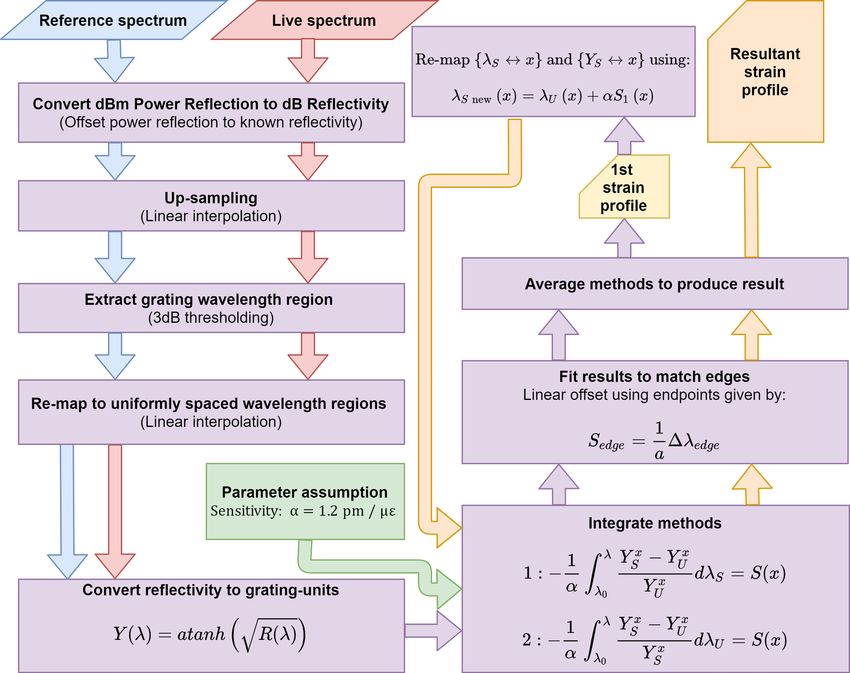
www.nature.com/scientificreports/
� S (x) d S (xS ) dS(xS )
≈ =β+α = β + αωx , (4d)
�xS dxS dxS
where we define the strain/temperature gradients: ωx = dS(x
dxS and ω =
S) dS(xS ( S ))
d S .
The reflectivity R β as a function of wavelength is obtained using the measured reflection spectrum from
an optical spectrum analyser. It is then transformed to ‘coupling strength–grating length’ product units by the
following:
x β
dx β
−1
(5)
Y β = tanh R β ∝ ≈ A x β ,
β d β
where A x β is an arbitrary variation factor that accounts for amplitude and grating-strength variation along
the grating.
Variation in the intensity-spectrum independent to the wavelength-shift of the CFBG from sources such as
amplitude variation from the light source, connection losses and fibre bend losses are assumed to be static and
have not been accounted for in the formulation.
The following requires that xU ( U ) = xS ( S ) = x such that the mapping { U ↔ x ↔ S } exists, which thus
requires:
S (x) = U (x) + αS(x), (6a)
d U
= 1 − αω , (6b)
d S
Defining U and S measurements respectively, we have YU|S ≡ Y U|S (x) as functions of
U|S U|S
≡ YU|S
their Bragg wavelengths expressed in x, and YU|S
x ≡ Y x (x) ≡ Y x as functions of x expressed in
U|S U|S x U|S
their Bragg wavelengths. From applying (5) to (4a–d), it follows that:
YSx − YUx
= −αω , (7a)
YUx
YSx − YUx −αω
x = , (7b)
YS 1 − αω
YS − YU −αωx
= , (7c)
YU β + αωx
YS − YU α
= − ωx , (7d)
YS β
Integrating (7a–d) against wavelength using (4a–d) and (6b) as substitutions, the strain/temperature pertur-
bation can be recovered as follows:
1 YSx − YUx
− d S = ω d S = S(x), (8a)
α YUx
0 0
1 YSx − YUx ω
− d U = (1 − αω )d S = ω d S = S(x), (8b)
α YSx 1 − αω
0 0 0
x x
1 YS − YU ωx ωx
− d S = d S = (β + αωx )dx = ωx dx = S(x) (8c)
α YU β + αωx β + αωx
0 0 x0 x0
x x
1 YS − YU 1 1
− d U = ωx d U = ωx βdx = ωx dx = S(x), (8d)
α YS β β
0 0 x0 x0
Since the typical experimental data YUx (x( U )) and YSx (x( S )) exists in wavelength domain, (8a) and (8b) are
used to perform the integration numerically, where (8a) is integrated against S and (8b) against U . By treating
the edge-points like regular FBGs, the strain/temperature at the endpoints is used to re-fit the integral result to
match the endpoint on both sides, using a linear offset. The { S ↔ x} map is required to form the { U ↔ x ↔ S }
map for the integration but since the perturbation remains unknown, the { S ↔ x} map is also unknown and
Scientific Reports | (2021) 11:1410 | https://doi.org/10.1038/s41598-020-80838-5 3
Vol.:(0123456789)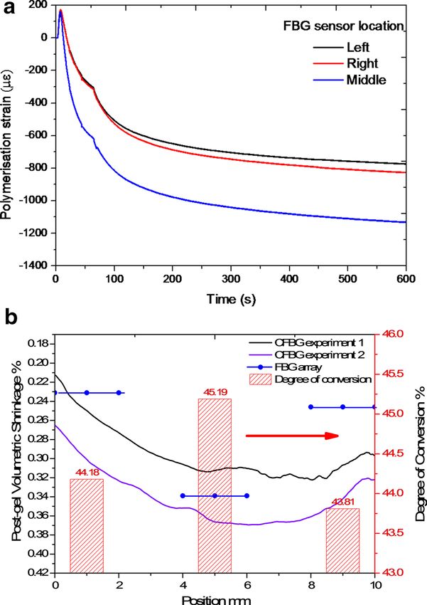
www.nature.com/scientificreports/
Figure 1. A flowchart of the process involved in measuring strain/temperature profile from a CFBG.
is given an initial 1-to-1 map between the two. By setting the number of data points or segments in U and S
as the same, each step along the integration corresponds to the same step in x for both YUx and YSx if { S ↔ x} is
known. The result from the integration of (8a) and (8b) will have slightly different results due unknown { S ↔ x}.
The results of both are averaged to create the result of the first integration which we shall denote S1 (x), which is
used to remap { S ↔ x} via (6a) such that:
S new (x) = U (x) + αS1 (x), (9)
From (9) the new map is given as follows:
new map : {x ↔ Snew }
define xnew : {xnew ↔ S } = {x ↔ Snew }
The new position variable xnew is then used to remap the YS values. The values are forced back into the same
original position variable as opposed to using the new position:
new map : {YS ↔ xnew }
defineYSnew : {YSnew ↔ x} = {YS ↔ xnew }
This ensures the position variable remains shared between the unperturbed and perturbed data during the
integration. Subsequently, YSnew and Snew replace their old counterparts in integrating (8a) and (8b). The out-
come of both are averaged to produce a more accurate result. This process can be repeated indefinitely, but in
practice, appear to converge extremely slowly so only one additional pass is necessary. The whole IOD process
and data processing is demonstrated in Fig. 1.
Experimental arrangement to measure the strain profile of a dental composite using the
developed method. The capability of the CFBG to measure the strain profile accurately by implement-
ing the IOD approach is demonstrated through a dental composite PS profile measurement. The test material
used in the study was a commercial photo-cured resin-based composite Beautifil FO3 (from Shofu Inc.). As the
polymer degree of conversion and the resultant PS of the material depend on the intensity profile of the curing
Scientific Reports | (2021) 11:1410 | https://doi.org/10.1038/s41598-020-80838-5 4
Vol:.(1234567890)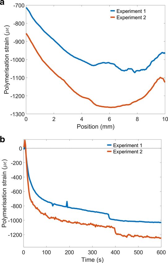
www.nature.com/scientificreports/
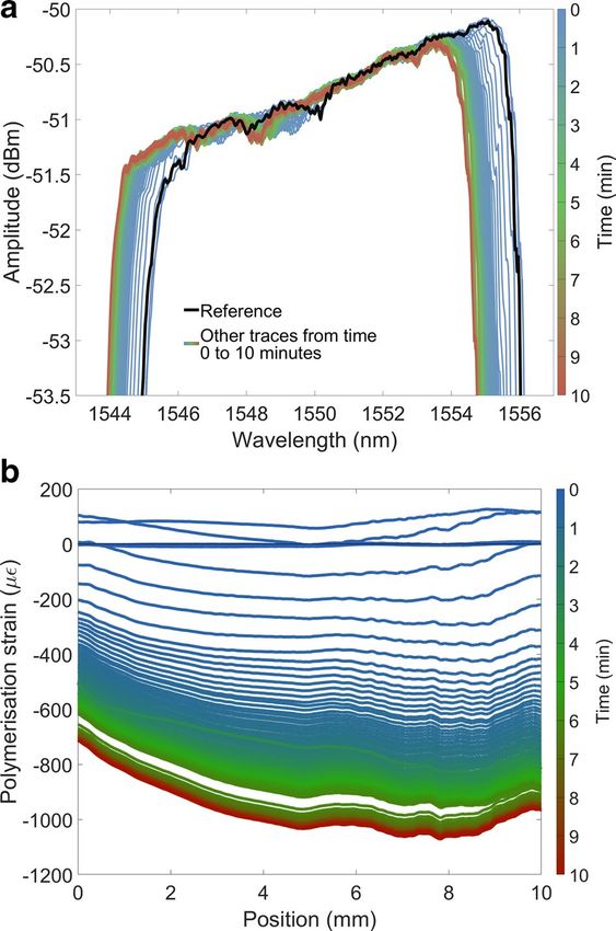
Figure 2. (a) Schematic experimental arrangement, (b) photograph of the setup.
lamp, we aim to measure resultant PS which could reflect the characteristics of the intensity distribution of the
curing lamp.
The CFBGs used are 10 mm long, centred at 1550 nm with a bandwidth of ~ 10 nm, at > 90% reflectivity
and recoated in polyimide. The optical fibre containing CFBG is fixed between two micro-blocks placed circa
200 mm apart with the optical fibre magnetically clamped on them. A custom made cylindrical Teflon mould
with 14 mm in diameter, 2 mm depth, with 1 mm depth grooves cut into the sides for placing the optical fibre
in was used for specimen manufacture. The 10 mm CFBG is placed at the middle region of 14 mm diameter
mould. After the optical fibre containing the CFBG and composite are placed in, the glass slide is placed flat on
top and ready for curing. Once this process is completed the CFBG spectrum is recorded for 5 min (~ 100 data
points) and averaged to produce the reference spectrum. Reference spectrum is recorded for 5 min to ensure that
CFBG is properly settled within the composite and its spectrum is stable. The test composite material was then
photo excited for 20 s by the curing lamp (X-Lite-II) and using the embedded CFBG at a depth circa 1 mm from
the surface of the material, the dynamic PS strain is measured for another 10 min. The spectrum analyser used
for measurement was Thorlabs OSA202C, which has a spectral resolution of ~ 50 pm at 1550 nm. Figure 2a,b
shows the experimental arrangement.
The reflectivity-spectrum was measured by setting the maximum measured intensity from the reference spec-
trum to the known reflectivity of the CFBG. Both the reference and live data are linearly interpolated by a factor
of 5 to artificially obtain a higher wavelength resolution for finding the edges of the CFBG region accurately,
obtained by thresholding 3 dB from the maximum. However, for spectrum analysers with high spectral resolu-
tion the linear interpolation may be skipped. The extracted regions of the live data are then linearly interpolated
again to fit the same wavelength domain and data size as the extracted reference. These values from the live and
reference are then used to perform the IOD.
To compare the results from the CFBG sensor, an FBG array with three sensors is also embedded in the dental
composite and PS strain at three locations are obtained—average strain across a 3 mm region centered at 3 mm,
7.5 mm and 13 mm of the 14 mm diameter dental composite specimen. All the experiments were conducted
separately, however, the experimental conditions were kept the same to obtain comparable results. The DC of
the material at the close proximity of the FBG sensor locations was also measured using FTIR technique to
understand the correlation between curing lamp intensity and polymerisation strain/shrinkage.
Results and discussion
One dimensional strain profile of a test biomaterial (dental composite). The measured poly-
merisation strain profile across the diagonal length of the composite from two repeated experiments conducted
is shown in Fig. 3a. The measured PS strain profile shows higher shrinkage at the middle region and lower
towards the edges, though an asymmetry is observed in the profile. Figure 3b shows the curing response in
the middle region of the composite specimen (at 5 mm position on the CFBG). The initial spike in the result is
due to a thermal rise from the curing exotherm and the curing lamp energy. Direct FBG peak wavelength shift
compensation alone cannot be used to discern between temperature and strain effects and thus a temperature
compensation technique would be needed to eliminate this spike, which is not considered in this study. The PS
slope observed is typical of photo-cured composites, where circa 75% of the PS occurs within the first 10 min
of curing35. Approximately a maximum of 200 με difference is observed (at 5 mm point of the CFBG) in the PS
strain between the two experiments which could be due to the difference in the embedment depth of the CFBG
Scientific Reports | (2021) 11:1410 | https://doi.org/10.1038/s41598-020-80838-5 5
Vol.:(0123456789)www.nature.com/scientificreports/
Figure 3. (a) PS strain profile of the dental composite measured using CFBG sensor, (b) PS strain response at
5 mm location of the dental composite specimen measured by the CFBG.
within the composite. Multiple experiments also showed that PS strain of the same material with the same
experimental setup yield similar results with an experimental error of circa 15%. However, this can be overcome
by using appropriate experimental setup where the embedment depth of the CFBG can be accurately set for all
experiments. Spikes and step changes in strain are also seen in the curing response (Fig. 3b), which is attributed
to minor delamination/debonding/jittering of the embedded optical fibre during the curing process. However,
this will only have minimal influence on the overall result and is ignored in the current study.
The spectral changes of the CFBG during the curing process and the PS strain profile evolution within the
dental composite for first 10 min is shown in Fig. 4a,b respectively. This gives an overview on how the curing
process is undertaking in the entire diagonal region of dental composite, rather than the average shrinkage for
the material obtained by other traditional methods. The curing rate is higher for initial phase (~ first 200 s) for
the entire region and then slows down and become stable within 10 min. From this data (Fig. 4b) the curing
characteristics of the material at any point along the length of the CFBG can be obtained as shown at 5 mm
position in Fig. 3b.
The asymmetry in the shape of the measured PS strain profile could be attributed to a variety of causes. The
CFBG region spans 10 mm whilst the marked region on the optical fibre containing the CFBGs (commercial
CFBG) used were 14 mm. Though we assume the CFBG is in the centre of the marked region, the exact location
of the CFBG within the fibre was unknown and its placement within the mould might be slightly off-centre with
the worst case error of ± 2 mm. Another plausible cause for the asymmetry is a poor endpoint selection where the
wavelengths used for the IOD process is outside the CFBG region. The tailing artefact observed at the end sup-
ports this hypothesis as well since the tailing may be from performing the IOD outside the CFBG region where
there is no experimentally induced wavelength-shifts and thus simply a noise-level amount of measured strain.
A poor endpoint selection also leads to a poor edge-point wavelength shift measured and thus poor endpoint
values used to re-fit the curve. This issue can be solved by having short 1 mm FBG sensors at both sides of the
CFBG, which be used as CFBG edge references.
The PS strain results from the CFBG is also compared with that of an FBG array embedded in the dental com-
posite where the average PS strain across a 3 mm region centered at 3 mm (left region), 7.5 mm (middle region)
and 13 mm (right region) of the dental composite specimen is measured. The PS strain response measured by
Scientific Reports | (2021) 11:1410 | https://doi.org/10.1038/s41598-020-80838-5 6
Vol:.(1234567890)www.nature.com/scientificreports/
Figure 4. (a) Changes in the CFBG spectra due to PS strain, (b) evolution of PS strain within the dental
composite for a duration of 10 min from cure initiation measured by the CFBG sensor.
the FBG array is shown in Fig. 5a where the average strain centered at 3 mm and 13 mm approximately corre-
sponds to the strain at the left (0–2 mm position) and right edges (8–10 mm position) of the CFBG respectively
and strain measured by the FBG at 7.5 mm corresponds to the strain measured by centre region of the CFBG
(4–6 mm position). Post-gel volumetric shrinkage of the specimen is estimated from the PS strain measured by
both CFBG and FBG array sensors assuming the material is isotropic is shown in Fig. 5b. FBGs measure average
post-gel volumetric polymerisation shrinkage of 0.23%, 0.34% and 0.25% for the left, centre and right regions,
whereas the CFBGs recorded an average (of two experiments across the same length of the FBG) of 25%, 34%
and 31% for the same region. The degree of conversion of the material at the FBG array locations was also meas-
ured and is also shown in Fig. 5b, where the PS strain is proportional to DC, which is influenced by the curing
lamps’ intensity characteristics. The results from the CFBG and FBG arrays are comparable and exhibits similar
trend. More accurate and precisely controlled experimental conditions such as depth of optical fibre within the
material, position of the sensor would yield a more comparable result.
The results from the FBG array and CFBG demonstrate that by using a single CFBG sensor, distributed
shrinkage strain profile (one dimensional/cross sectional) of the material can be obtained and can reduce the
complexity associated with FBG arrays which provides similar results with less spatial resolution. Furthermore
in this work only one CFBG is used as a proof-of-concept demonstration, however having multiple CFBGs, 2D
or 3D strain profiles of the material can be obtained which would not be possible by any other means.
Potential clinical benefits of the new PS profiling method. The developed approach has many
potential clinical benefits. To facilitate the development of innovative dental composites/biomaterials, a better
understanding of their characteristics and curing response is required, from micro to macro scales. The ability to
photo-cure composite resins is based on position and orientation of the curing light and its radiant e nergy2. Cur-
rently available curing lights vary in many aspects such as different tip diameter, intensity and irradiance which
will affect the resultant cure outcomes. As such the physical characteristics of the material, which are a function
of the curing light characteristics, therefore, would be different in laboratory test conditions and in clinical appli-
cations. One common approach adopted by practitioners and curing light manufacturers is to increase the light
intensity and irradiance, so that under any circumstances, the composite resin is photo activated well. The ISO
standard limit the irradiance to 200 mW/cm2 for the wavelength region of 190–380 nm, however, most of the
Scientific Reports | (2021) 11:1410 | https://doi.org/10.1038/s41598-020-80838-5 7
Vol.:(0123456789)www.nature.com/scientificreports/
Figure 5. (a) PS strain response at three locations of the dental composite measured by the FBG array, (b)
comparison of post-gel volumetric PS of the dental composite measured by CFBG sensor and FBG sensor array.
commercial curing light’s spectral distribution is beyond 380 nm and have irradiance up to 2000 mW/cm2 36,37.
This itself possess a significant health hazard to the patients and the practitioners. The excess heat generated by
the curing light, and the exothermic reaction of the composite resin, will affect the tooth pulp and soft tissues38,39.
So simply increasing the irradiance is not the solution to the problem. The solution is to understand the
response of the composite resin towards the curing light characteristics and optimise the composite-light system.
Having the shrinkage profile information of the composite across specimen and its correlation with curing lamp
intensity will allow the clinicians to work more informed and to modify/improve their restoration techniques
which will improve their longevity.
Conclusion
We have demonstrated an IOD based approach for interrogation of a CFBG for distributed strain measurements
or strain profile mapping. As a proof of concept of the developed approach the technique was applied to PS
strain profile measurement of photo-cured dental composites. The successful results show potential use of this
technology for shrinkage profile mapping of polymer-based biomaterials and composites. The technique requires
refinement to mitigate strain-gradient errors and further work for 2D/3D strain profiling.
Data availability
The data that support the findings of this study are available from the corresponding author upon reasonable
request.
Received: 4 September 2020; Accepted: 22 December 2020
References
1. Xu, X., He, L., Zhu, B. & Li, J. Advances in polymeric materials for dental applications. Polym. Chem. 8, 807–823 (2017).
2. Rueggeberg, F. A., Giannini, M., Arrais, C. A. G. & Price, R. B. T. Light curing in dentistry and clinical implications: a literature
review. Braz. Oral Res. 31, e61 (2017).
3. Watts, D. C., Marouf, A. S. & Al-Hindi, A. M. Photo-polymerization shrinkage-stress kinetics in resin-composites: methods and
development. Dent. Mater. 19, 1–11 (2003).
4. Maas, A. S. et al. Trends in restorative composites research: what is in the future?. Braz. Oral Res. 31, e55 (2017).
Scientific Reports | (2021) 11:1410 | https://doi.org/10.1038/s41598-020-80838-5 8
Vol:.(1234567890)www.nature.com/scientificreports/
5. Schneider, L. F. J., Cavalcante, L. M. & Silikas, N. Shrinkage stresses generated during resin-composite applications: a review. J.
Dent. Biomech. 2010, 131630 (2010).
6. Soares, C. J. et al. Polymerization shrinkage stress of composite resins and resin cements—what do we need to know?. Braz. Oral
Res. 31, e62 (2017).
7. Sunbul, H., Silikas, A. N. & Watts, D. C. Polymerization shrinkage kinetics and shrinkage-stress in dental resin-composites. Dent.
Mater. 32, 998–1006 (2016).
8. Opdam, N. J. M. et al. Longevity of posterior composite restorations: a systematic review and meta-analysis. J. Dent. Res. 93,
943–949 (2014).
9. Münchow, E. A., Meereis, C. T. W., de Oliveira da Rosa, W. L., da Silva, A. F. & Piva, E. Polymerization shrinkage stress of resin-
based dental materials: a systematic review and meta analyses of technique protocol and photo-activation strategies. J. Mech. Behav.
Biomed. Mater. 82, 77–86 (2018).
10. Guimarães, G. F. et al. Minimization of polymerization shrinkage effects on composite resins by the control of irradiance during
the photo activation process. J. Appl. Oral Sci. 26, e20170528 (2018).
11. He, J., Garoushi, S., Vallittu, P. K. & Lassila, L. Effect of low-shrinkage monomers on the physicochemical properties of experimental
composite resin. Acta Biomater. Odontol. Scand. 4, 30–37 (2018).
12. Lu, H., Lee, Y. K., Oguri, M. & Powers, J. M. Properties of a dental resin composite with a spherical inorganic filler. Oper. Dent. 31,
734–740 (2006).
13. Mitra, S. B., Wu, D. & Holmes, B. N. An application of nanotechnology in advanced dental materials. J. Am. Dent. Assoc. 134,
1382–1390 (2003).
14. Kwon, Y., Ferracane, J. & Lee, I. B. Effects of layering methods, composite type and flowable liner on the polymerization shrinkage
stress of light cured composites. Dent. Mater. 28, 801–809 (2012).
15. Ferracane, J. L. et al. Academy of Dental Materials guidance- Resin composites: Part ii- Technique sensitivity (handling, polymeri-
sation, dimensional changes). Dent. Mater. 33, 1171–1191 (2017).
16. Silikas, N., Eliades, G. & Watts, D. C. Light intensity effects on resin-composite degree of conversion and shrinkage strain. Dent.
Mater. 16, 292–296 (2000).
17. Rajan, G. et al. Polymerisation shrinkage profiling of dental composites using optical fibre sensing and their correlation with degree
of conversion and curing rate. Sci. Rep. 9, 3162 (2019).
18. Lau, A., Li, J., Heo, Y. C. & Fok, A. A study of polymerization shrinkage kinetics using digital image correlation. Dent. Mater. 31,
391–398 (2015).
19. Rajan, G. Optical Fibre Sensors: Advanced Techniques and Applications (CRC Press, Boca Raton, 2015).
20. Rao, Y. J. In-fibre Bragg grating sensors. Meas. Sci. Technol. 8, 355–375 (1997).
21. Rajan, G. & Prusty, B. G. Structural Health Monitoring of Composite Structures using Fiber Optic Methods (CRC Press, Boca Raton,
2016).
22. Ottevaere, H., Tabak, M., Chah, K., Mégret, P. & Thienpont, H. Dental composite resins: measuring the polymerization shrinkage
using optical fiber Bragg grating sensors. Proc. SPIE 8439, 843903 (2012).
23. Anttila, E. J. et al. Evaluation of polymerization shrinkage and hydroscopic expansion of fiber-reinforced biocomposites using
optical fiber Bragg grating sensors. Dent. Mater. 24, 1720–1727 (2008).
24. Kashyap, R., McKee, P. F., Campbell, R. J. & Williams, D. L. Novel method of producing all fibre photoinduced chirped gratings.
Electron. Lett. 30, 996–998 (1994).
25. Imai, T., Komukai, K. & Nakazawa, M. Dispersion tuning of a linearly chirped fiber Bragg grating without a center wavelength
shift by applying a strain gradient. IEEE Photonics Technol. Lett. 10, 845–847 (1998).
26. Feng, K. M. et al. Dynamic dispersion compensation in a 10-Gb/s optical system using a novel voltage tuned nonlinearly chirped
fiber Bragg grating. IEEE Photonics Technol. Lett. 11, 373–375 (1999).
27. Bettini, P., Guerreschi, E. & Sala, G. Development and experimental validation of a numerical tool for structural health and usage
monitoring systems based on chirped grating sensors. Sensors 15, 1321–1341 (2015).
28. Korganbayev, S. et al. Detection of thermal gradients through fiber-optic Chirped Fiber Bragg Grating (CFBG): medical thermal
ablation scenario. Opt. Fiber Technol. 41, 48–55 (2018).
29. Palumbo, G., Tosi, D., Iadicicco, A. & Campopiano, S. Analysis and design of Chirped fiber Bragg grating for temperature sensing
for possible biomedical applications. IEEE Photonics J. 10(3), 1–15 (2018).
30. Tosi, D. Review of chirped fiber Bragg gratings (CFBG) fiber-optic sensors and their applications. Sensors 18, 2147 (2018).
31. Kitcher, D. J., Nand, A., Wade, S. A., Jones, R., Baxter, G. W. & Collins, S. F. Implementation of integration of differences method
for extraction of temperature profiles along chirped fibre Bragg gratings. In ACOFT/AOS 2006 - Australian Conference on Optical
Fibre Technology/Australian Optical Society. 57–59, (2006).
32. Tosi, D. Review and analysis of peak tracking techniques for fiber Bragg grating sensors. Sensors 17, 2368 (2017).
33. Saccomandi, P. et al. Linearly chirped fiber Bragg grating response to thermal gradient: from bench tests to the real-time assess-
ment during in vivo laser ablations of biological tissue. J. Biomed. Opt. 22, 097002 (2017).
34. Kashyap, R. Fiber Bragg Gratings (Academic Press, London, 1999).
35. Feilzer, A. J., De Gee, A. J. & Davidson, C. L. Curing contraction of composites and glass-ionomer cements. J. Prosthet. Dent. 59,
297–300 (1988).
36. Price, R. B., Labrie, D., Whalen, J. M. & Felix, C. M. Effect of distance on irradiance and beam homogeneity from 4 light emitting
diode curing units. J. Can. Dent Assoc. 77, b9 (2011).
37. Price, R. B., Labrie, D., Bruzell, E. M., Sliney, D. H. & Strassler, H. E. The dental curing light: a potential health risk. J. Occup.
Environ. Hyg. 13, 639–646 (2016).
38. Mouhat, M., Mercer, J., Stangvaltaite, L. & Örtengren, U. Light-curing units used in dentistry: factors associated with heat devel-
opment-potential risk for patients. Clin. Oral Investig. 21, 1687–1696 (2017).
39. Park, S. H., Roulet, J. F. & Heintze, S. D. Parameters influencing increase in pulp chamber temperature with light-curing devices:
curing lights and pulpal flow rates. Oper. Dent. 35, 353–361 (2010).
Acknowledgements
This research was supported by the Australian Research Council (ARC) Linkage Project (LP160100260) and
AusIndustry CRC-Project (CRCPSEVEN000013).
Author contributions
G.R. and A.W. conceived the idea and implemented the concept. Experimental works were carried out by A.W.
and G.R. G.R., A.W., P.F. and B.G.P. took part in the analysis and discussion. G.R. and A.W. drafted the paper
and all authors contributed to the writing.
Scientific Reports | (2021) 11:1410 | https://doi.org/10.1038/s41598-020-80838-5 9
Vol.:(0123456789)www.nature.com/scientificreports/
Competing interests
The authors declare no competing interests.
Additional information
Correspondence and requests for materials should be addressed to G.R.
Reprints and permissions information is available at www.nature.com/reprints.
Publisher’s note Springer Nature remains neutral with regard to jurisdictional claims in published maps and
institutional affiliations.
Open Access This article is licensed under a Creative Commons Attribution 4.0 International
License, which permits use, sharing, adaptation, distribution and reproduction in any medium or
format, as long as you give appropriate credit to the original author(s) and the source, provide a link to the
Creative Commons licence, and indicate if changes were made. The images or other third party material in this
article are included in the article’s Creative Commons licence, unless indicated otherwise in a credit line to the
material. If material is not included in the article’s Creative Commons licence and your intended use is not
permitted by statutory regulation or exceeds the permitted use, you will need to obtain permission directly from
the copyright holder. To view a copy of this licence, visit http://creativecommons.org/licenses/by/4.0/.
© The Author(s) 2021
Scientific Reports | (2021) 11:1410 | https://doi.org/10.1038/s41598-020-80838-5 10
Vol:.(1234567890)You can also read