Calibration strategy for the SPICA/SAFARI instrument - arXiv
←
→
Page content transcription
If your browser does not render page correctly, please read the page content below
Calibration strategy for the SPICA/SAFARI instrument
                                                  Russell F. Shipmana , Bart Vandenbusscheb , Edgar Castillo-Domingueza , Alvaro Labianoc ,
                                                                           Willem Jellemaa , and Angiola Orlandoa
                                                                            a
                                                                         SRON, Landlevel 12, Groningen, Netherlands
                                                                                   b
                                                                                     KUL, Leuven, Belgium
                                                   c
                                                     Centro de Astrobiologı́a (CAB, CSIC-INTA), ESAC Campus, E-28692 Villanueva de la
                                                                                    Cañada, Madrid, Spain

                                                                                                ABSTRACT
                                               SPICA is a mid to far infra-red space mission to explore the processes that form galaxies, stars and planets.
arXiv:2101.04473v1 [astro-ph.IM] 12 Jan 2021

                                               SPICA/SAFARI is the far infrared spectrometer that provides near-background limited observations between 34
                                               and 230 micrometers. The core of SAFARI consists of 4 grating modules, dispersing light onto 5 arrays of TES
                                               detectors per module. The grating modules provide low resolution (250) instantaneous spectra over the entire
                                               wavelength range. The high resolution (1500 to 12000) mode is accomplished by placing a Fourier Transform
                                               Spectrometer (FTS) in front of the gratings. Each grating module detector sees an interferogram from which the
                                               high resolution spectrum can be constructed. SAFARI data will be a convolution of complex spectral, temporal
                                               and spatial information. Along with spectral calibration accuracy of < 1 %, a relative flux calibration of 1% and
                                               an absolute flux calibration accuracy of 10% are required. This paper will discuss the calibration strategy and
                                               its impact on the instrument design of SAFARI
                                               Keywords: Grating spectrometer, Fourier transform spectroscopy, TES bolometers

                                                                                           1. INTRODUCTION
                                               SPICA (SPace Infrared telescope for Cosmology and Astrophysics), one of three remaining candidates for the
                                               ESA Medium Class M5 mission and due to compete for the M5 slot through ESA’s Mission Selection Review
                                               process starting in early 2021, was unexpectedly cancelled by ESA in October 2020 on financial grounds. With
                                               an actively cooled 2.5m-diameter telescope, this space observatory would have comprised three instruments
                                               (SAFARI – SpicA FAR-infrared Instrument, SMI – SPICA Mid-Infrared Instrument and B-BOP – magnetic
                                               field (B) explorer with BOlometric Polarimeter) working in synergy to provide unprecedented spectroscopic and
                                               photometric sensitivity in the mid- and far-infrared, transforming infrared astronomy in fields ranging from
                                               planet formation to star formation through to studies of the interstellar medium and galaxy evolution.
                                                  This paper/poster is one in a series of SPIE contributions from the SPICA Consortium that is aimed at
                                               preserving the technological developments and knowledge gained through work undertaken by many scientists
                                               over several years, ensuring that the legacy of SPICA is not lost through the untimely cancellation of this mission.
                                               Further details on the SPICA mission are discussed in ”The joint infrared space observatory SPICA: Unveiling
                                               the obscured universe”.1
                                                  The SPICA Far Infrared Spectrometer (SAFARI) will improve on the spectral line sensitivity of previous
                                               missions (the Herschel and Spitzer space telescopes) by taking advantage of a cold telescope and unprecedentedly
                                               sensitive detectors.2 Being a very sensitive spectrometer SAFARI reveals the physical phenomena occurring
                                               within an obscured environment. SAFARI opens the window to the very distant Universe as well as nearby star
                                               and planet formation.
                                                   Calibration of SAFARI is challenging. SAFARI is exceptionally sensitive, but planets and stellar calibrators
                                               within the detection range of earlier far-infrared space observatories will easily saturate the very sensitive de-
                                               tectors. At 8K, the cold primary will have emission only at the longest wavelengths. A deep integration on a
                                                  Further author information: (Send correspondence to R.F, Shipman)
                                                  R.F. Shipman.: E-mail: R.F.Shipman@sron.nl ,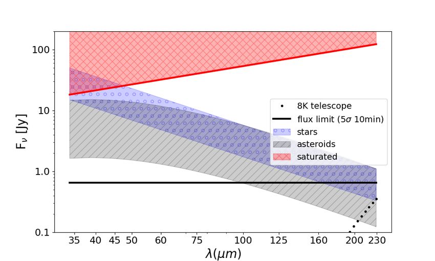
distant galaxy will detect the local foreground emission of the zodiacal dust cloud and the Galactic emission
which must be removed. Observing faint line emission on bright continua from nearby proto-planetary disks will
likely show non-linearity effects.
We outline the key components necessary to calibrate the SAFARI instrument. This article is organized
as follows: section 2 describes the SPICA mission and SAFARI instrument. In section 3 we present a concep-
tual operation of SAFARI. Section 4 describes the calibration requirements and section 5 outlines how those
requirements could be met. A summary of the main points is presented in section 6.
2. SAFARI DESCRIPTION
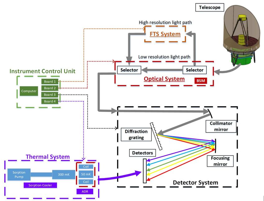
The SPICA Far Infrared Spectrometer (SAFARI)3 is a dual resolution grating spectrometer, combined with a
high resolution post dispersed Fourier Transform Spectrometer. A simplified version of the conceptual design
can be seen in Figure 1. The design is simple: an optical system selects if the light beam from the telescope is
directly coupled to a detector system (low resolution light path, LR), or the beam is first directed to a Fourier
Transform Spectrometer (high resolution light path, HR). The mode selector is the mechanisms which controls
which path is used.
Figure 1. Conceptual design of SAFARI. A selectable low/high resolution spectrograph/spectrometer is proposed to
comply with the two different resolutions required by key SAFARI science questions. The beam steering mirror (BSM)
together with the mode selector and the calibration source (not shown) make up the optical system.
The LR sends the light to a spectrometer with diffraction gratings as dispersing elements. Diffraction gratings
were selected to minimize the loss of light in the materials due absorption and dispersion. The gratings are
designed to provide an optical resolution in the spectral axis of 250. In the HR, the light passes first through a
Fourier Transform Spectrometer, then through the grating spectrograph. This post dispersion operation increases
the spectral resolution up to the range between 1500 to 12000, depending on the wavelength range (34 µm to
230 µm) and also reduces the background photon noise by dividing the incoming light into all detectors.
An important component of the optical system is the beam steering mirror (BSM). It has two main functions,
one is to direct the incoming radiation from the telescope to a specific point in the focal plane, the other is todirect the radiation from an internal calibration source to the focal plane. The focal plane has a 2 × 2 square
arcminutes field of view (FOV).
Because of the high bandwidth required, along with absolute accuracy and uniformity along the whole band
in both intensity and spectral measurements, it was decided to divide the spectral range in 4 sections, one for
each of the 4 grating modules. In this way, four different optimizations are possible in optical performance, mass,
volume and accommodation in the available space on SPICA.
In each of the 4 grating modules the dispersed optical signal is recorded by 5 arrays of TES bolometers
with a sensitivity close to background-limited.2 The 5 arrays record spatially different signals from the sky but
are co-aligned across the grating modules. Each array of 147 individual bolometers constitutes a spaxel, each
spectral element (bolometer) in the spaxel is a spectral pixel. Figure 2 demonstrates the layout and the steps
of an observation. A single spaxel produces a spectrum sampled once per resolution element. To achieve two
samples per spectral resolution element (Nyquist sampling), the arrays are offset by a fraction of a spectral
resolution element. For example spaxels 1, 3 and 5 would be offset by 1/2 a resolution element. A beam steering
mirror (BSM) is used to direct the input signal from a given sky direction onto a desired spaxel. Modulating
the signal with the BSM between spaxel 3 and 1 (or 3 and 5), would allow for a fully sampled spectrum to be
recorded. In Figure 2, the BSM steers the beam from the target onto spaxel 3 and then spaxel 1 and back. Thus
modulating the signal. The other spaxels receive signal near but off the target which is taken to be background.
As seen in Figure 3, the background is measured at the same time as the target at positions between about 40
to 100 arcseconds off target.
Grating modules are co-aligned on the sky, spaxel 1 of grating module 1 sees the same sky position as spaxel
1 of grating modules 2,3 and 4. The final product of SAFARI are fully sampled spectra from 34 to 230 microns.
Figure 3 shows the footprint of SAFARI on the sky. The circles represent the SAFARI beams (in full width at
half maximum, FWHM) from 34 µm to 230 µm. This figure shows the spatial offset between spaxels. Each
spaxel has ≈ 40 arcsec separation from the next.
3. OBSERVING MODES
SAFARI measures spectra with either low resolution gratings (LR mode) or high resolution (HR mode) by
inserting an FTS in front of the gratings (see Figure 1).
3.1 Low resolution single spectra
Consider an emission source with spectral flux density Sν , an instrument response function Fν and a spaxel
dependent aperture efficiency ηj .
Assuming a linear detector’s response, the measured flux density of a source in LR mode over the pixel i is:
R
∆ν
Sν Fν ηj dν
Sij = R ij (1)
F η dν
∆νij ν j
where the integral is over the bandwidth ∆ν of the ith pixel of spaxel j. Each pixels sees a bandwidth ∆ν in
either the LR mode or the HR mode.
LR spectra of a single objects are a major scientific mode for SAFARI. The purpose of this mode is to measure
fully sampled low resolution spectrum (near λ/∆λ = 250). Begin background limited, One of SAFARI’s main
science goals is to measure the interstellar medium (ISM) in distant galaxies.
SAFARI is designed to always integrate on source. The BSM places the target on one spaxel, while the other
4 spaxels see nearby (40-100 arcseconds) off background. The BSM then switches the target to a different spaxel.
Thus an integration is a modulation between target and nearby background. In Figure 2 when the BSM is in
position one, the target emission falls on the middle spaxel, when the BSM shifts to position two the middle
spaxel receives radiation from the background.
The spaxels will be offset from each other also in the dispersion direction by a fraction of a spectral resolution
element. With spectrally offset spaxels (1/2 a spectral resolution element), the final spectrum is created byBSM position 1
BSM position 2
Figure 2. Layout of detector arrays in one grating module. Each detector is shown as a blue rectangle. A row of pixels
make up a spaxel. Detector rows probe a spectral segment for 5 positions offset in the sky. The detector row (spaxel)
centered on the target in the sky is highlighted with a box.
Note, all spaxels are receiving sky background radiation, only the central spaxel is receiving radiation from the target.
Figure 3. Focal plane footprint on sky. This figure shows the full width at half maximum of the shortest (center of each
circle) and longest wavelength (large circles) pixels of the 5 spaxels assuming Gaussian beams at each wavelength.
interlacing the integrations from two different spaxels. Due to construction of a linear TES array within a
grating module there will be gaps in the spectral coverage between TES bolometers. The interlacing also fills
these spectral gaps.
Each pixel is modulated by chopping between an ON target position and an OFF target position. The power
measured within a pixel-bandwidth, ∆νi , while ON target, Pi,ON , is a combination of power from the target in
∆νi , the power from the foreground emission in ∆νi and the ”power” registered with no loading due to the bias
voltage of the pixel, Pi,0 :
Pij,ON = Pij,target + Pij,bkga + Pij,0 (2)
Pij,OF F = Pij,bkgb + Pij,0 (3)The subscript ij refers to the ith pixel of spaxel j. Both Pij,bkga and Pij,bkgb are due to foreground emission.
As can be seen from Figure 3, the background positions are separated by about 80 arcseconds on the sky. For
most diffuse background sources (Zodiacal emission or Galactic dust emission) there will not be any significant
spatial variation over within a few arcminutes, hence Pij,bkga ≈ Pij,bkgb . In case the background emission is
highly variable, the chopping can be performed more symmetrically by making use of more spaxels (chopping
from spaxel 3 to 1 then 3 to 5) and interpolating to determine the background emission Pbkga . Furthermore, the
background emission is broadband continuum emission and nearby pixels within a spaxel at different wavelengths
can also be used to determine the background power. The power from the target is:
∆Pij = Pij,ON − Pij,OF F = Pij,target + Pij,bkga − Pij,bkgb ≈ Pij,target (4)
However, as stated earlier, the spectrum of the target should be sampled twice. The modulation steps in
represented in Equation 4 observe the source only once within the bandwidth of the pixel. We therefore make
use of the spaxel which is chopped onto the the position of the target j + 2 or j − 2.
Pij±2,ON = Pij±2,target + Pij±2,bkga + Pij±2,0 (5)
Here again i refers to the it h pixel of spaxel j + 2 or j − 2.
∆Pij±2 = Pij±2,target (6)
Interleave the signals of pixel i from the different spaxels gives the final spectrum:
Sλ = I(λ)[Pij,target , Pij±2,target ] (7)
Where I(λ) reconstructs (interpolates) the interleaved target signal.
3.1.1 Low resolution mapping
Some of SAFARI’s key science questions also call for a spectral mapping mode. Small raster maps could be made
using the pointed mode described above but at different positions on the sky. The BSM can cover a 2’x2’ field of
view to produce a small map. Larger maps could be made by stitching smaller maps together. A more efficient
On-The-Fly mapping scheme is also possible. In this mode, SAFARI is integrating while the telescope slews.
3.2 High resolution single spectra
As described in section 2, the mode selector is used to redirect the telescope beam through the FTS in high
resolution mode (HR). In the HR mode, each detector produces an interferogram Sij (t) during the scanning of
the FTS mechanism over time t, such that the Fourier Transform produces the spectrum of the source :
Sij (ν) = F T (Sij (t)) (8)
The FTS mechanism is then scanned its length and back. Given 4 grating modules each with 5 spaxels of
roughly 150 pixel, a single FTS scan will produce roughly 3000 interferograms.
If more than one scan is required for the proper integration, either the BSM or a re-pointing of the satellite
can be used to place the target on a different spaxel to address the small band gaps between pixels.
4. CALIBRATION REQUIREMENTS
When linear, the voltage modulation of pixel i in spaxel j is directly related to the absorbed power:
Pij = Kij ∆Vij (9)
Where Kij depends pixel, spaxel, BSM position and potentially if the source is extended or point-like.Table 1. Calibration items which follow from requirements and dependency for pixel i, spaxel j
Item name Item label pixel, spaxel, BSM Requirement %
Wavelength calibration λ i, j 1.0
Flat-field FF i, j, x 0.1
Relative flux calibration RSRF i, j, λ 1.0
Absolute flux Calibration Fcal λ 10
Cross talk Xtalk i, j < 0.1
4.1 Calibration items
Table 1 lists the calibration items that are needed to address the requirements. The table identifies the depen-
dencies of the calibration item on wavelength (λ), pixel (i), spaxel (j) or BSM position (x). The BSM allows
for different optical paths through the SAFARI optics which could have a calibration impact. The BSM also
provides a position on the primary which may be at a slightly different temperature.
4.2 Wavelength/frequency calibration
In LR mode, instrument level testing (ILT) provides most of the wavelength calibration. Both the grating and
the pixels are stationary. This can be determined in laboratory testing and is not expected to change. However
the calibration should be confirmed in flight.
In HR mode determining the frequency calibration is more involved. The high resolution is achieved with
an FTS where the optical path difference (OPD) creates an iterferogram. The Fourier Transform of that inter-
ferogram is the source signal. The OPD must be accurately determined at all time steps during the scan of the
FTS mechanism. One key component is the zero path difference (ZPD) when there is no difference in the path
lengths between the two arms. There will be almost 3000 pixels which can be used to help determine ZPD.
4.3 Spectral line-shape
While not a specific calibration requirement, spectral line-shapes should be determined across the frequency
range of SAFARI. In the LR mode, a spectral line is observed by two spaxels and spread over multiple pixels.
The observation over different spaxels requires interlacing of the final spectrum and proper interpolation onto
a finer wavelength grid. The line-shape will be measured towards external sources with unresolved lines and
compared with the instrument simulator.4
The spectral lines are observed and constructed via signals from slightly paths through the optics: the BSM
is used to redirect the source signal to a different spaxel (see Figure 2). Any BSM dependence on the response
will have to be measured/modelled.
In the HR mode, the spectral line shape is determined by the spectral response of the pixel itself. Again, the
comparison with the instrument model should be made to raise confidence that the instrument and response are
well understood.
SAFARI will observe brighter nearby proto-planetary disks. For these sources, the line shape will be de-
pendent on correcting any non-linear response of the detectors while making the interferogram. A proper
measurement and monitoring of the non-linear response of the detectors will be needed.
4.4 Relative flux calibration
The relative flux calibration refers to the flux calibration of each pixel relative to the other pixels. For pixels
close in wavelength , the requirement is 0.1% in LR mode. IN HR the requirement is 1%.
The relative response functions of the detectors will be mapped during ILT. The ILT measurements are
required throughout the mission for proper calibration. ILT measurements provide the spectral/spatial of each
bolometer.The internal calibration source provides a stable reference for extended emission. It will not provide infor-
mation regarding point source coupling. But it will aid in monitoring SAFARI as a whole.
In flight, the RSRF will be verified using calibration standards, both stellar and broadband continuum sources.
4.4.1 Low resolution RSRF
The main calibration parameter for the relative flux calibration is to determine the response relative to adjacent
pixels. In this sense the low resolution RSRF is more akin to a flat-field. An internal calibration source that
provides a stable featureless extended signal will be key for determining and monitoring the flat-field (see Section
5.2). Broadband continuum point sources will be needed to determine a point source correction to the flat-field.
Detailed modelling of SAFARI is necessary to determine if there will be a position dependence and how sensitive
to pointing errors the flat-field/RSRF will be.4
4.4.2 High resolution RSRF
In HR mode, a major calibration step will be the creation of a ”clean” interferogram before Fourier trans-
forming5 .6 Each pixel creates an interferogram. This provides redundancy and an opportunity to examine the
interferograms for instrumental correlations which otherwise would impact the quality of the data.
Within the bandwidth of a pixel, a properly corrected interferogram has the most impact on the relative
response. Broad bandwidth FTS spectrometers like SPIRE required special processing steps to deal with the
changing beam size,7 the bandwidth over a grating pixel is small enough not to show beam size issues between
pixels. Observations of broadband sources like asteroids should provide both RSRF and absolute calibrations.
Monitoring of the RSRF in high resolution will be performed with observations of the internal calibration
source (see Section 5.2).
The RSRF in high resolution mode is a measure of the response at frequencies within the bandpass of each
pixel. The determining of the ”flat-field” as described above will remain import for proper spectral stitching
across the entire SAFARI wavelength range.
4.5 Absolute flux calibration
Absolute flux calibration will rely on observing well modelled celestial sources. Traditionally, these sources have
been a combination of stars, planets and minor planets. Unfortunately, Uranus and Neptune have flux densities
greater than a few hundred Jy in SAFARI wavelength range and are all too bright (Figure 4).
Herschel observed stars, planets and minor planets as flux calibrators.8 Sources such as γDra are observable
with SAFARI as are asteroids and minor planets.
Figure 4, shows a top level overview of possible calibrators. The figure identifies two limits. The top hatched
area identifies at which flux density level SAFARI will likely saturate. High resolution observations saturate
at roughly twice the limit. The lower solid line indicates the flux level that can be achieved in a 10 minute
observation (5σ). To be a viable calibration source, the object should observable in a relatively short amount
of time. The dimmest star in the diagram, γ Dra, makes it clear that no single star is usable across the entire
SAFARI range, but some asteroids would be.
5. CALIBRATION STRATEGY
Calibration activities take place on different time scales. The observing mode must first and foremost guarantee
that integrating on a source will reduce the observed noise. This is achieved by periodically monitoring the
system gain by flashes of the calibration source. Data from these flashes will be used to bring every observation
to a standard level. This is not an absolute flux calibration, but a link between normal operations and the
absolute flux calibrators described below.
Another requirement from the system is to produce a properly sampled spectrum. Properly sampled fulfills
the Nyquist sampling requirement of at least two samples per resolution bandwidth. In the low resolution mode
of grating data, this is accomplished by the spaxel arrays being offset from each other by a fraction of a spectral
resolution element. This is shown in Figure 2. In high resolution mode the FTS fulfills the requirement by
design.5.1 Pre-flight characterization
During instrument level testing (ILT), many calibration parameters will be determined. Among these will be the
actual layout of the focal plane as-built. In combination with the grating, this layout determines the wavelength
calibration.
ILT will also map the focal plane in the spatial and spectral dimensions. This map results in the relative
spectral response (RSRF) for each detector in every spaxel of all four grating modules. When combined with a
telescope model, the RSRF is the instrument response to incoming radiation. This will result in roughly 3000
response functions. Mapping of the focal plane should also include checks of how impact of the BSM on the
RSRF and whether any corrections are needed when combining (interlacing) signals from two different BSM
positions.
Another outcome of the RSRF mapping above will be a cross talk matrix. Likely, there will be cross talk
given the frequency domain multiplexing. Depending on the layout of the multiplexing (all within a spaxel
or across spaxels), identifying cross-talk in-flight could be very difficult. A laboratory measurement will be
necessary. Specifically important for bright sources will be determining the non-linear response. Over a wide
dynamic range, the detector response is linear, but timing effects appear once the source brightness approaches
saturation. Being intrinsic to the detector/readout system, the non-linearity is not expected to change once
measured. Although that should be verified in-flight.
One final ILT activity will be to determine the stability of various components of the SAFARI instrument.
Higher stability elements require less frequent calibration activities and increase the overall instrument efficiency.
The stability analysis will specify the cadence of calibrations.
5.2 Internal calibration source
The internal calibration source is present to provide a stable consistent signal across all SAFARI wavelengths. It
can be used to monitor the overall response of the system as well as monitor the response gain by providing signals
which modulate between two power levels. Such a ”flash” signal was key to the SPIRE response monitoring and
calibration scheme for both their photometers and FTS spectrometer,9 .10 The current design of the calibration
source makes use of two micro-lamps in an integration sphere. These lamps produce black-body radiation at two
different temperatures. The signal produced from the two lamps is a broad, featureless spectrum covering the
entire range of SAFARI and illuminating all 5 spaxels.
The useful time scale of the calibration source is per observation to daily. As a monitoring component, the
internal source will be used to bring the entire SAFARI response to a standard time in order to bootstrap the
absolution calibration to the entire mission.
The SAFARI internal calibration source will need to have the following capabilities.11
• Standard spectroscopic source signal. This should be a flat spectral signal that illuminates the entire
wavelength range of SAFARI as well as the 5 spaxels. This signal can be used to monitor the relative
response of SAFARI in HR mode.
• Small modulated signal. This is also a flat signal covering the entire SAFARI range, but can be modulated
between two levels. This signal will be used to monitor the gain of the detector system in both LR and HR
modes. In HR mode, the FTS mechanism will have to be set at ZPD and then modulate the calibration
source (see Section 4.2).
• Dark signal. When off, the calibration source will be at the 4K and provide a dark reference signal.
• Comb spectrum. In a separate mode, the calibration source can provide a comb signal for frequency
calibration of the FTS. This will not only be useful for frequency calibration of the FTS, but will also
contribute to the wavelength calibration in low resolution mode since the FTS requires the grating to
disperse the signal into finer bandpasses.
• Saturating source possibility. For monitoring purposes, one potential capability for the calibration source
would be to produce a signal which partially saturates the instrument. This provides a check over time of
any fundamental changes in the instrument.5.3 External calibrators
External calibrators are needed for wavelength calibration, line shape, relative and absolute flux calibration.
To verify the wavelength calibration, SAFARI will observe external narrow line sources such as planetary
nebulae (PN). The key here will be to find sufficiently weak PN that will not saturate SAFARI but bright
enough to be observed in a reasonable time (see Figure 4). Being solely determined by the focal plane layout,
the wavelength calibration is not expected to vary over the mission. This still should be measured. Observations
of narrow line sources like PN will also determine, in-flight, the spectral line shape for both LR and HR modes.
Figure 4 shows the flux ranges where external flux calibrators will be used. The top boundary indicates where
SAFARI would be saturated. The black line indicates the 5σ flux limit in LR mode for a 10 minute integration.
To keep calibration time to a minimum and maximize efficiency, integration times on calibration sources should
be relatively short. The lower bound for stars is based on the star γDra. As can bee seen this will not saturate,
but at long wavelengths, the integration time will be a concern. In general stellar sources vary significantly
across the SAFARI range making them less than ideal. Asteroids are potentially a better option, since they can
be proper point sources with flat spectra. In the coming years effort should be invested in understanding these
sources and improving the models.
Figure 4. External calibrators. SAFARI can make use of some standard absolute flux calibrators. It would be good
to expand the potential list. The saturation level is identified as the red square-hatch area. Neptune and Uranus fall
into this region as does Ceres. The stellar calibration shows a range (in blue circles) of standard established calibrators
from γ Dra to α Boo. The asteroid range shown in grey hatches is within a factor of 3 of the faintest asteroid calibrator
considered for Herschel: Lutetia.8
6. SUMMARY
In this note the calibration requirements and strategy for the SAFARI instrument have been discussed. The
main conclusions are as follows:
• SPICA/SAFARI will have roughly 3000 distinct spectral elements. Each one requires spectral, spatial and
non-linearity characterisation.
• Many of the characterisation will be performed during ILT. This will help confirm instrument simulations.• SAFARI will make use of a very simple but highly repeatable internal calibration source, not for absolute
calibration but rather to monitor the performance.
• The extraordinary sensitivity of the SAFARI’s TES detectors make the instrument susceptible to saturation
from standard established external calibrators such as planets and many stars.
• The broad simultaneous wavelength range of SAFARI makes it challenging to find external calibrators
which have sufficient flux at all wavelengths but do not saturate.
• In the coming years, the list of external calibrators in the far infrared needs to be expanded. Likely objects
will be asteroids, but also more distant planetary nebula and AGB stars. The stellar flux calibrator network
for JWST - extending mid-infrared calibration networks to fainter targets - is a promising starting point.
The next generation of far infrared instruments will make use of the technological advances in detector
technology of the past decades. The advances have been significant and have substantially increased sensitivity,
linearity and dynamic range. The SPICA/SAFARI instrument would have been one of these major advances
by taking advantage of a cold large telescope and the most sensitive detectors. SAFARI does not image the far
infrared sky but rather measures in exquisite detail the rich far infrared spectrum.
ACKNOWLEDGMENTS
R.S. thanks David Naylor for many useful discussions and his insight to the needs of an FTS. A.L. acknowledges
the support from Comunidad de Madrid through the Atracción de Talento grant 2017-T1/TIC-5213. This
research has been partially funded by the Spanish State Research Agency (AEI) Project MDM-2017-0737 Unidad
de Excelencia “Marı́a de Maeztu”- Centro de Astrobiologı́a (INTA-CSIC).
REFERENCES
[1] Roelfsema, P. R., Shibai, H., Kaneda, H., Sauvage, M., Najarro, F., Bradford, C. M., Yamada, T., Tauber,
J., Audard, M., Doi, P. D. Y., Elbaz, D., Griffin, M., Helmich, F., Heske, A., Honda, M., Jellema, W.,
Juvela, M., Kamp, I., Kerschbaum, F., Kiss, C., Kohno, K., Krause, O., de Lange, G., Larsson, B., Martı́n-
Pintado, J., Hideo Matsuhara, T. N., Nagao, T., Naylor, D., Nomura, H., Ogawa, H., Onaka, T., Rouquet,
J., Spinoglio, L., Szczerba, R., van der Tak, F., Vandenbussche, B., and Wang, S.-Y., “The joint infrared
space observatory spica: Unveiling the obscured universe,” in [Space Telescopes and Instrumentation 2020:
Optical, Infrared, and Millimeter Wave (Conference 11443)], Proc. SPIE 11443(11443-205) (2020).
[2] Audley, M. D., de Lange, G., Gao, J.-R., Jackson, B. D., Hijmering, R. A., Ridder, M. L., Bruijn, M. P.,
Roelfsema, P. R., Ade, P. A. R., Withington, S., Bradford, C. M., and Trappe, N. A., “The safari detector
system,” in [Milimeter, Submillimeter and Far-Infrared Detectors and Instrumentation for Astronomy IX)],
Proc. SPIE 107080(107080K) (2018).
[3] Roelfsema, P. R., Dieleman, P., Jellema, W., de Lange, G., Evers, J., Giard, M., Najarro, F., Bradford,
C. M., Audard, M., Doi, Y., Griffin, M., Helmich, F., Juvela, M., Kerschbaum, F., Kiss, C., Krause, O.,
Larsson, B., Naylor, D., Spinoglio, L., Szczerba, R., van der Tak, F., Vandenbussche, B., and Wang, S.-
Y., “The safari grating spectrometer for spica: Extreme spectroscopic sensitivity in the far-ir,” in [Space
Telescopes and Instrumentation 2020: Optical, Infrared, and Millimeter Wave (Conference 11443) ], Proc.
SPIE 11443(11443-231) (2020).
[4] Jellema, W., Spinoglio, L., Pascale, E., Savini, G., Fernandez-Ontiveros, J., Causi, G. L., Shipman, R.,
Griffin, M., Naylor, D., and van Loon, D., “The spica-safari instrument and scientific performance simula-
tor,” in [Space Telescopes and Instrumentation 2020: Optical, Infrared, and Millimeter Wave (Conference
11443) ], Proc. SPIE 11443(11443-225) (2020).
[5] Fulton, T., Naylor, D. A., Polehampton, E. T., Valtchanov, I., Hopwood, R., Lu, N., Baluteau, J. P.,
Mainetti, G., Pearson, C., Papageorgiou, A., Guest, S., Zhang, L., Imhof, P., Swinyard, B. M., Griffin, M. J.,
and Lim, T. L., “The data processing pipeline for the Herschel SPIRE Fourier Transform Spectrometer,”
Monthly Notices Royal Astronomical Society 458, 1977–1989 (May 2016).
[6] Davis, S. P., Abrams, M. C., and Brault, J. W., [Fourier transform spectrometry ], Academic Press (2001).[7] Wu, R., Polehampton, E. T., Etxaluze, M., Makiwa, G., Naylor, D. A., Salji, C., Swinyard, B. M., Ferlet,
M., van der Wiel, M. H. D., Smith, A. J., Fulton, T., Griffin, M. J., Baluteau, J. P., Benielli, D., Glenn,
J., Hopwood, R., Imhof, P., Lim, T., Lu, N., Panuzzo, P., Pearson, C., Sidher, S., and Valtchanov, I.,
“Observing extended sources with the Herschel SPIRE Fourier Transform Spectrometer,” Astronomy and
Astrophysics 556, A116 (Aug. 2013).
[8] Müller, T., Balog, Z., Nielbock, M., Lim, T., Teyssier, D., Olberg, M., Klaas, U., Linz, H., Altieri, B.,
Pearson, C., Bendo, G., and Vilenius, E., “Herschel celestial calibration sources. Four large main-belt
asteroids as prime flux calibrators for the far-IR/sub-mm range,” Experimental Astronomy 37, 253–330
(July 2014).
[9] Bendo, G. J., Griffin, M. J., Bock, J. J., Conversi, L., Dowell, C. D., Lim, T., Lu, N., North, C. E.,
Papageorgiou, A., Pearson, C. P., Pohlen, M., Polehampton, E. T., Schulz, B., Shupe, D. L., Sibthorpe, B.,
Spencer, L. D., Swinyard, B. M., Valtchanov, I., and Xu, C. K., “Flux calibration of the Herschel SPIRE
photometer,” Monthly Notices Royal Astronomical Society 433, 3062–3078 (Aug. 2013).
[10] Swinyard, B. M., Polehampton, E. T., Hopwood, R., Valtchanov, I., Lu, N., Fulton, T., Benielli, D., Imhof,
P., Marchili, N., Baluteau, J. P., Bendo, G. J., Ferlet, M., Griffin, M. J., Lim, T. L., Makiwa, G., Naylor,
D. A., Orton, G. S., Papageorgiou, A., Pearson, C. P., Schulz, B., Sidher, S. D., Spencer, L. D., van der
Wiel, M. H. D., and Wu, R., “Calibration of the Herschel SPIRE Fourier Transform Spectrometer,” Monthly
Notices Royal Astronomical Society 440, 3658–3674 (June 2014).
[11] Wu, E. S.-Y. W., Wang, M.-J., Chen, T.-J., Chang, Y.-P., Huang, Y.-R., Wang, C.-L., Chiu, C.-P., Pei,
T.-H., Evers, J., Arrazola, D., Eggens, M., Martin, S., and Jellema, W., “The calibration source assembly for
spica/safari instrument,” in [Space Telescopes and Instrumentation 2020: Optical, Infrared, and Millimeter
Wave (Conference 11443) ], Proc. SPIE 11443(11443-216) (2020).You can also read


