Predicting regional coastal sea level changes with machine learning
←
→
Page content transcription
If your browser does not render page correctly, please read the page content below
www.nature.com/scientificreports
OPEN Predicting regional coastal sea level
changes with machine learning
Veronica Nieves*, Cristina Radin & Gustau Camps‑Valls
All ocean basins have been experiencing significant warming and rising sea levels in recent decades.
There are, however, important regional differences, resulting from distinct processes at different
timescales (temperature-driven changes being a major contributor on multi-year timescales). In view
of this complexity, it deems essential to move towards more sophisticated data-driven techniques
as well as diagnostic and prognostic prediction models to interpret observations of ocean warming
and sea level variations at local or regional sea basins. In this context, we present a machine learning
approach that exploits key ocean temperature estimates (as proxies for the regional thermosteric
sea level component) to model coastal sea level variability and associated uncertainty across a range
of timescales (from months to several years). Our findings also demonstrate the utility of machine
learning to estimate the possible tendency of near-future regional sea levels. When compared to
actual sea-level records, our models perform particularly well in the coastal areas most influenced by
internal climate variability. Yet, the models are widely applicable to evaluate the patterns of rising and
falling sea levels across many places around the globe. Thus, our approach is a promising tool to model
and anticipate sea level changes in the coming (1–3) years, which is crucial for near-term decision
making and strategic planning about coastal protection measures.
Short-term variations in regional coastal sea levels depend on a combination of nearshore and offshore processes,
including fast-paced changes like those associated to high tides or storms and interannual to multi-year changes
driven by relatively large temperature oscillations (thermosteric variations) in large open ocean areas—just
to name a few1. More particularly, open ocean, temperature changes down the water column to 700 m depth
are still influencing regional coastal sea level variability changes2,3, and they are closely tied to internal natural
climate variability4–6. Internal climate variability due to natural fluctuations of the ocean–atmosphere coupled
system (such as the Pacific Decadal Oscillation) can lead to periods when the upper ocean warms more slowly
or more rapidly, which has direct implications for sea level c hange6. Nevertheless, climate is a highly complex
and networked dynamical system (with no simple relationships) that can change naturally in unexpected w ays7,8.
From this perspective, advanced statistical analyses, including machine learning (ML) methods, can provide
useful insight.
In recent years, ML techniques have provided significant advances in the modeling of physical variables at
both global and local scales9–11. These techniques can help identify complex relationships between explanatory
variables, and, at the same time, establish “relevance metrics” (i.e. ranking of the level of importance of each
variable). This way, we can optimally combine multiple data towards explainability and prediction of events.
However, efforts to develop and implement these techniques in the context of the ocean to forecast short-term
changes, including near-future regional sea-level predictions, remain largely u nexplored12–15.
In this study, we aim to perform a comprehensive evaluation of thermal expansion in open ocean regions
driving changes in coastal sea levels to model and pinpoint the “tendency” of increase/decrease in sea level for
the next years. Rather than using physics-based equations to describe such changes, our ML models are informed
by upper-ocean temperature proxy estimates which, in turn, reflect the underlying physics (e.g., ocean dynamics
and internal variability)3. The analysis was done by assessing the specific role of the different elements (including
different oceanic depth layers and timescales) with nonlinear ML algorithms. Contributions of land movements,
changes in tidal range and storm surges to relative sea level were excluded from the analysis. Our innovative
approach (Fig. 1) has been tested in 26 coastal regions surrounding the Pacific, Indian, and Atlantic basins. As
demonstrated in the case studies, the large temperature fluctuations (by short-term climate changes and ocean
circulation) are dominating the patterns of sea level variability changes for most of the regions.
Image Processing Laboratory, University of Valencia, Valencia, Spain. *email: veronica.nieves@uv.es
Scientific Reports | (2021) 11:7650 | https://doi.org/10.1038/s41598-021-87460-z 1
Vol.:(0123456789)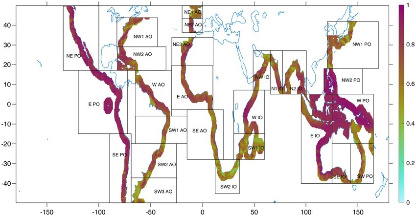
www.nature.com/scientificreports/
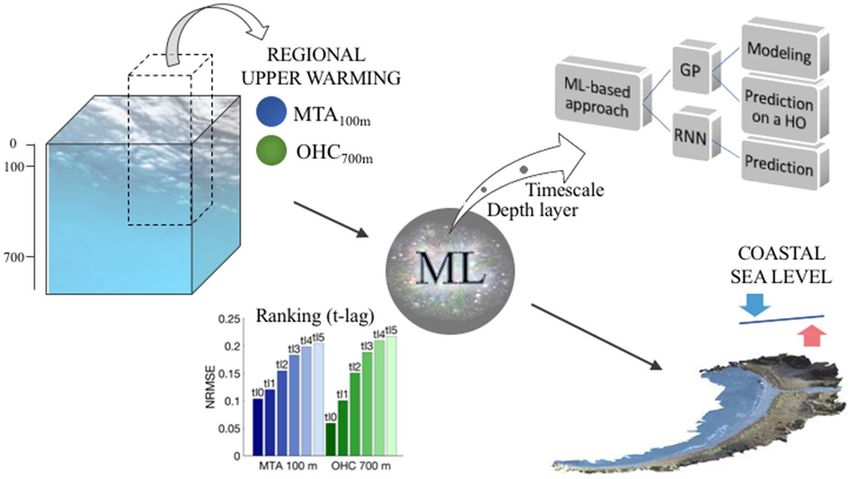
Figure 1. Illustration of our ML approach. The proposed approach combines physical variables (that reflect
upper-ocean temperature changes) in open ocean regions and ML techniques (i.e., the nonlinear GP and RNN
methods) to assess coastal sea level variability in these regions across a range of timescales. This framework
includes a relevance criterion to rank the physical variables according to their performance modeling such
changes, while also considering different time lags (Figs. S1-S4).
Figure 2. Correlation map between the regional (GP) model and observed sea level estimates at each location
of the regions indicated in the boxes and 1993–2018 period. For each specific coastal location, we considered the
neighboring data grid points as well, using a weighting local (scaling) function, to account for possible offsets
from data31. The map was generated using the software MATLAB (version 2019a) http://www.mathworks.com/
products/matlab/.
Results and discussion
ML helps modeling regional sea level variability changes. To model sea level variations in the coastal
regions from upper-ocean temperature changes in the open ocean (a proxy for climate variability conditions), we
first calculate the median estimate within each ocean region (Fig. 2) for each variable (sea level anomaly, SLA;
vertically averaged temperature anomaly, MTA; depth-integrated temperature or heat content, OHC) over the
period 1993–2018 (see Materials and Methods). Note that the various temperature-based estimates (MTA and
OHC) were calculated across different depth layers (i.e. from 0 to 100 and 700 m depth). Since the patterns of
both MTA 700 m and OHC 700 m are deemed similar16,17, we only show the latter (as well as MTA 100 m) here.
Scientific Reports | (2021) 11:7650 | https://doi.org/10.1038/s41598-021-87460-z 2
Vol:.(1234567890)www.nature.com/scientificreports/
A B C
100 100 100
50 50 50
0 0 0
-50 -50 -50
-100 -100 -100
1993 2001 2009 2018 1993 2001 2009 2018 1993 2001 2009 2018
Observed Modeled (GP)
Predicted (GP HO) Predicted 1 yr (RNN) Predicted 2 yr (RNN) Predicted 3 yr (RNN)
Figure 3. The regional modeled and predicted patterns are consistent with observed sea level variability.
(A) Time series of the GP model (in blue) and observed sea level estimates (black) for the west Pacific Ocean
region (shown in Fig. 2). (B) Same as in A but here the holdout method was used to predict sea level for the last
3 years of the record (in gray) by training the GP model from 1993 to 2015. (C) Sea level predictions for 1 (red),
2 (purple) and 3 (orange) years using the RNN method by training the observed sea level estimates (black)
from 1993 to 2017, 2016 and 2015, respectively. The shaded envelops depict 95% prediction intervals. Sea level
expressed in mm.
The study domain covers the tropical to mid-latitudes (50°S to 50°N). However, our main goal is to investigate
low-latitude sea level changes induced by natural regimes of variability, which operates away from the melting
glaciers and other effects18. In addition, records have been detrended and smoothed to emphasize interannual
to multi-year variability. However, only analyses of data smoothed with a 3-year moving average filter are given
here by way of example (see Supplementary Information for results at other timescales). Also point out that
we defined relatively wide ocean regions chosen for their significant climate patterns, like the Pacific Decadal
Oscillation (PDO), the North Atlantic Oscillation (NAO) or the Indian Ocean Dipole (IOD), or for their physi-
cal regimes (i.e., large-scale transport dynamics), such as in the Kuroshio‐Oyashio Extension or the Agulhas
Current (Fig. 2). Similar results were observed considering slightly different regions.
Our first target was to use Gaussian Processes (GPs) to determine spatiotemporal relationships between the
temperature estimates (MTA and OHC) in the open sea regions and the coastal SLA estimates of these regions, as
our intention was to also highlight the influence of the open ocean on the c oast19. GPs are versatile ML methods
for non-parametric nonlinear regression with prediction uncertainty20, which typically yields good accuracy
results in the g eosciences9,21. In the model configuration, time-lagged responses were considered as well as dif-
ferent oceanic depth layers (as indicated above). The resulting models (for each region, depth layer, time-lag and
timescale) are called the “sea-level proxies”. To further understand the features of the proxies, and analyze their
performance, the following measures were used: the root mean square error (RMSE), which was normalized by
the difference between the maximum and minimum value, and the explained variance (EV), i.e., the coefficient
of determination ( R2) (see Materials and Methods).
Based on the outcome metrics (Fig. S3), it was found that the depth average temperature over the top 100 m
(i.e. MTA 100 m) was enough to characterize sea level variability changes in the regions within tropical latitudes
(e.g., E PO, W AO, SW1 AO, SE AO, W/NW IO). The east Atlantic domain (i.e., E AO) and the Indo-Pacific
basin (from the west Pacific warm-pool to the north and east Indian Ocean, i.e., NW2 PO, W PO, E IO, N1/
N2 IO) are the exception, as the heat uptake in these regions can extend up to 700 m depth22,23. In these cases,
therefore, a temperature estimate that includes the upper 700 m (e.g., MTA 700 m or OHC 700 m) would be
a more suitable choice to capture the thermal expansion information. It is also interesting to note that, in the
subtropical regions, MTA/OHC 700 m usually works better in the northern hemisphere, and MTA 100 m in the
southern sites. Regardless of the region, generally, results do not show any time lag between our estimates and
the SLA, also with few exceptions. For example, in the west and southwest Indian Ocean (W and SW2 IO) and
northeast Atlantic Ocean (NE1/2 AO) the highest performance is achieved when a time lag is considered. This
means that, in these regions, sea level changes can be detected in advance.
The time series shown in Fig. 3A correspond to the model obtained from one of the highest ranked tempera-
ture estimates (Fig. S3), compared against the observational-based sea level estimates for the west Pacific Ocean
region (see Supplementary Information for the other regions). We chose this region for illustration purposes
as it shows large sea level variations linked to oceanic mixed-layer heat content8,24. This region, which includes
Indonesia’s islands, is also among the locations most threatened by rising sea levels1. We can see, however, that
overall the observed and modeled sea level estimates agree well in all regions influenced by low‐frequency climate
variability, such as in the Indo-Pacific region (i.e., E IO, NW2 PO, W PO) and along the east Pacific coast (i.e.,
NE/E/SE PO). This also includes the western Indian (W IO) and central Atlantic oceans (W and E AO, extending
into the NW2 AO and NE3 AO). In these regions, our GP model can explain at least 70% of the total variance,
Scientific Reports | (2021) 11:7650 | https://doi.org/10.1038/s41598-021-87460-z 3
Vol.:(0123456789)www.nature.com/scientificreports/
and correlation values range from 0.84 to 0.97 (see Fig. S7). In the other regions, the model performance differs
between good (NE2 AO, NW IO, N2 IO, SE IO) and fairly good (SW PO, SW1 AO, N1 IO, NW1 AO) with cor-
relation values higher than 0.80 and 0.70, respectively, excluding some regions where their climate conditions and
local characteristics play a key role. The highest biases are found, for example, in the regions with mid-latitude
wind-driven circulation, such as western boundary currents (e.g., SW2 IO, NW1 PO, SW2 and SW3 AO)18.
Regions with high variance also coincide with places where salinity changes can be really large (as large as the
thermosteric contribution, e.g., NE1 AO, SW1 IO or NW1 PO)25, or where there exists a combination of several
effects (like in the SE AO)26. Even so, our model still offers a relatively good performance with regional correla-
tion values always higher than 0.62. While this may vary at specific site locations (see Fig. 2), results suggest that
the upper-thermal changes are still considerably impacting the regions and timescales studied here (Figs. S5-S8).
Complementary analysis of other aspects (e.g., vertical land motion, tidal effects, storms, land ice change) could
be performed to help better interpret results where relevant.
Towards short‑term predictions. We conducted further analysis using the GP model performed on a
holdout set. This allows us to investigate, in particular, if by training the model using a certain percentage of
the data, namely 88.5% (i.e., the 23 first years, from 1993 to 2015), we can construct the forecasting model with
the remaining (11.5% of the) data (i.e., the last 3 years, from 2016 to 2018) (Materials and Methods). As seen in
Fig. 3B and in Figs. S9-S12 (Supplementary Information), we found that, in general, the variability lies within the
95% prediction intervals. Therefore, our GP-based approach not only has the ability to identify regional coastal
sea level variability changes from proxy data, but it could also be exploited in the future for filling data gaps
(when information is missing or uncertain) and for proxy reconstructions of past sea level (1955–1993) changes.
Nevertheless, even if the holdout method embeds a predictive response, it has its limitations when it comes to
prediction of future changes as it uses a fraction of the full data for both training and predicting.
Hence, towards modeling and assessing sea-level predictions up to several years into the future, we imple-
mented an alternative ML algorithm based on recurrent neural networks (RNNs), the long short-term memory
(LSTM) (see Materials and Methods). This method has demonstrated excellent capabilities in learning real-world
data that exhibits complex nonlinear patterns, especially, but not only, in the Earth s ciences11,27. Unlike the GP
method, the distinct advantage of the RNN method is that it can capture dynamic behavior and accounts for
memory effects in the model’s architecture. This allows the model to perform forecasting beyond the in-sample
training dataset without using additional data. To train the model we introduced a (training/validation) parti-
tion using the observed sea level data. We reserved a portion (the last years) of the historical record to test the
robustness of predictions. Given the relatively limited length of the altimetry record, we only used one year for
validation and up to three years for testing predictions. As expected, we observed that the model was often able
to provide more accurate predictions for one to two years in advance, as opposed to three (see Figs. S13-S16 in
Supplementary Information). However, in the particular case of the west Pacific Ocean, the rise in sea level was
detected in all conducted experiments (Fig. 3C). It is also no surprise that, again, there are some regions (NW1
PO, SW1 and SW2 IO, SE AO, SW2 and SW3 AO) where sea levels are more difficult to predict, consistent with
the above results. We believe, however, that the model could be improved by using more data when it becomes
available. Noting that, in many cases, our model revealed correctly the magnitude of change (in relation to the
1993 baseline), even though our target was to simply detect the (positive/negative) tendency towards an increase/
decrease in future regional sea levels.
Results show that both the GP and RNN models are promising ML techniques for automatically modeling and
predicting short-term regional coastal sea level changes. Furthermore, the flexibility of the proposed framework
to analyze multiple data enables the possibility to explore in the future other proxy variables or a combination
of them.
Conclusion
Machine learning-based strategies for predicting the nonlinear behavior of short-term regional coastal sea level
changes are still rarely present. Our machine learning approach has shed new light on this problem in two ways.
One on hand, it has allowed to mimic sea level variability changes to a large extent in many coastal regions around
the Pacific, Indian and Atlantic oceans, by establishing physical relationships between input temperature variables
from the upper layers of open ocean regions (that play a decisive role in regional “thermosteric” expansion) and
sea level estimates at the coastal sites of these regions. Beyond that, it has been possible to provide reasonably
accurate region-specific predictions of the sea level tendency for one to two/three years. Thereby, the introduced
methodology offers a view that is not purely statistical, and also fills the gap between the coastal adaptation plan-
ners demand and the existing multidecadal-to-century projections of sea level change.
Materials and methods
Observational datasets. Two sources of observational-based data were analyzed: (i) daily satellite mean
sea level anomalies (SLA) through 2019 (https://resources.marine.copernicus.eu/?option=com_csw&view=
details&product_id=SEALEVEL_GLO_PHY_L4_REP_OBSERVATIONS_008_047), resampled at seasonal
(3-month) resolution; (ii) seasonal in-situ-based vertically-averaged temperature anomalies for the 0–100 m
and 0–700 m layers (MTA 100 m, MTA 700 m) and heat content for the 0–700 m layer (OHC 700 m) through
present (https://www.nodc.noaa.gov/OC5/3M_HEAT_CONTENT/). These temperature-based estimates have
been demonstrated to have good quality through direct comparisons with field measurements and intercompar-
isons with other satellite-derived products28. All products have been expressed from their 1993–2018 mean and
smoothed with a 1-, 3-, and 5-year Savitzky-Golay filter29 (that smooths according to a quadratic polynomial that
is fitted over each window) to help distinguish natural internal fluctuations from the historical anthropogenic
Scientific Reports | (2021) 11:7650 | https://doi.org/10.1038/s41598-021-87460-z 4
Vol:.(1234567890)www.nature.com/scientificreports/
warming signal and assess multi-time-scale variability. To get the regional estimates, instead of estimating the
area-weighted average over each oceanic region (shown in Fig. 2), we chose the median v alue30, as it has a slightly
better regional representation, especially where the noise of interannual variability is high, as we have seen here.
Model experiments and evaluation. For our modelling and prediction experiments, two machine learn-
ing techniques were used; a Gaussian process (GP) regression model and a recurrent neural network (RNN)
with long-short term memory (LSTM) units. The GPs are state-of-the-art non-parametric methods (and the
preferred choice) for machine learning regression, while RNNs apply recurrent operations to data in a neural-
network fashion to account for and forecast complex nonlinear dynamics.
The GP methods were used in two different ways. First, to generate the GP regression model, we trained
the different temperature input variables with the satellite altimetry sea level (1993–2018) record using the
MATLAB fitrgp function (with KernelFunction = Exponential, FitMethod = None, PredictMethod = Exact, as the
model specifications21). A lag of up to 15 months for the temperature input variables was selected following a
series of different time lags to explore a lagged-response between the temperatures and sea level estimates. As
the GP models are trained, we compute the mean squared error (MSE) to assess which input variables generally
performs best on each region. The coefficient of determination was also estimated to account for goodness-of-
fit: R2 = 1 − N ∗ 2 N
i=1 (yi − yi ) / i=1 (yi − ȳ) , where yi and yi are the observed sea level estimate and the model
2 ∗
prediction from the temperature data, respectively, for each region/location. Note that the right side of the equa-
tion represents what the model cannot explain, hence R2 (or explained variance, EV) should be interpreted as
the proportion of variability that is explained by the model. R , its square-root value, is equivalent to a measure
of correlation, indicating how strongly related the coupled patterns are. According to this performance criterion,
the variables are categorized in terms of rankings.
Alternatively, and the second use of GPs, the same sort of analysis could be performed on a holdout set to
test the predictive performance of the GP method using the highest ranked temperature estimates. With the
hold-out approach, we use a relatively high percentage of the (temperature and sea level) data for training a
new model (again using the fitrgp function) and this model with the rest of the (temperature) data to predict
outcomes (using the MATLAB predict tool). In this study, the partitioning of the dataset is not random but done
into consecutive periods of time to respect a certain date. We use the same metrics (EV and R) to assess robust-
ness of the model outputs.
An additional experiment was performed to explore the potential use of LSTMs/RNNs techniques to pre-
dict future sea-level tendencies. These techniques provide the possibility to take a set of data and train a model
which can be used to generate reasonable predictions without using another set of data to model from 11. In this
analysis, the RNN is directly trained against the sea level data using the MATLAB trainNetwork tool with the
below-specified training options and Long Short-Term Memory (LSTM) network architecture27. The predicted
responses were obtained by applying the MATLAB predictAndUpdateState function with the trained recurrent
neural network. This function also updates the network state at each prediction, giving it memory of previous
inputs. All hyper-parameters in the network were determined via cross-validation in the training set. The best
overall performance was obtained with the ‘adam’ solver (a good optimization algorithm for training a neural
network) and 4 layers with 2–20 hidden units. The hidden units allow the networks to produce a nonlinear
response to the inputs and represent “mean” predicted output. It was observed that fewer hidden units did not
fully learn the complexity of the patterns, and that additional hidden units could lead to overfitting the training
dataset. The number of epochs (i.e., the number of complete passes through the training set) is automatically set
by the above functions based on the loss calculation, so that the network will stop training when the loss on the
validation set has been equal to (or larger than) the previous smallest loss for several consecutive epochs, and
it differs among regions. The RMSE loss of each model run is hence used as the performance indicator for each
iteration. For this experiment, training datasets were split for training, validation and testing.
Received: 2 December 2020; Accepted: 30 March 2021
References
1. Intergovernmental Panel on Climate Change, in Climate Change 2013: The Physical Science Basis (eds Stocker, T. F. et al.) (Cam-
bridge Univ. Press, Cambridge, 2013).
2. Palanisamy, H., Cazenave, A., Delcroix, T. & Meyssignac, B. Spatial trend patterns in the Pacific Ocean sea level during the altimetry
era: the contribution of thermocline depth change and internal climate variability. Ocean Dyn. 65, 341–356. https://doi.org/10.
1007/s10236-014-0805-7 (2015).
3. Nieves, V., Marcos, M. & Willis, J. K. Upper-ocean contribution to short-term regional coastal sea level variability along the United
States. J. Climate 30, 4037–4045. https://doi.org/10.1175/JCLI-D-16-0896.1 (2017).
4. Cazenave, A., Dieng, H. & Meyssignac, B. The rate of sea-level rise. Nat. Clim. Change 4, 358–361. https://doi.org/10.1038/nclim
ate2159 (2014).
5. WCRP Global Sea Level Budget Group. Global sea-level budget 1993–present. Earth Syst. Sci. Data 10, 1551–1590. https://doi.
org/10.5194/essd-10-1551-2018,2018 (2018).
6. Hamlington, B. et al. Understanding of contemporary regional sea level change and the implications for the future. Rev. Geophys.
https://doi.org/10.1029/2019RG000672 (2020).
7. Cheng, L., Abraham, J., Hausfather, Z. & Trenberth, K. E. How fast are the oceans warming?. Science 363, 128–129. https://doi.
org/10.1126/science.aav7619 (2019).
8. Widlansky, M. J., Long, X. & Schloesser, F. Increase in sea level variability with ocean warming associated with the nonlinear
thermal expansion of seawater. Commun Earth Environ. 1, 9. https://doi.org/10.1038/s43247-020-0008-8 (2020).
9. Camps-Valls, G. et al. A survey on gaussian processes for earth observation data analysis: a comprehensive investigation. IEEE
Trans. Geosci. Rem. Sensing (2016). https://doi.org/10.1109/MGRS.2015.2510084
Scientific Reports | (2021) 11:7650 | https://doi.org/10.1038/s41598-021-87460-z 5
Vol.:(0123456789)www.nature.com/scientificreports/
10. Camps-Valls, G. et al. Physics-aware Gaussian processes in remote sensing. Appl. Soft. Comput. 68, 69–82. https://doi.org/10.
1016/j.asoc.2018.03.021 (2018).
11. Reichstein, M. et al. Deep learning and process understanding for data-driven Earth system science. Nature 566, 195–204. https://
doi.org/10.1038/s41586-019-0912-1 (2019).
12. Sztobryn, M. Forecast of storm surge by means of artificial neural network. J. Sea Res. 49, 317–322. https://doi.org/10.1016/S1385-
1101(03)00024-8 (2003).
13. Bajo, M. & Umgiesser, G. Storm surge forecast through a combination of dynamic and neural network models. Ocean Model 33,
1–9. https://doi.org/10.1016/j.ocemod.2009.12.007 (2010).
14. French, J., Mawdsley, E., Fujiyama, T. & Achuthan, K. Combining machine learning with computational hydrodynamics for predic-
tion of tidal surge inundation at estuarine ports. Procedia IUTAM 25, 28–35. https://doi.org/10.1016/j.piutam.2017.09.005 (2017).
15. Visser, H., Dangendorf, S. & Petersen, A. C. A review of trend models applied to sea level data with reference to the “acceleration-
deceleration debate”. J. Geophys. Res. Oceans 120, 3873–3895. https://doi.org/10.1002/2015JC010716 (2015).
16. Abraham, J. P. et al. A review of global ocean temperature observations implications for ocean heat content estimates and climate
change. Rev. Geophys. 51, 450–483. https://doi.org/10.1002/rog.20022 (2013).
17. Wunsch, C. Multi-year ocean thermal variability. Tellus A: Dyn. Meteorol. Oceanogr. 72, 1–15. https://doi.org/10.1080/16000870.
2020.1824485 (2020).
18. Hu, A. & Bates, S. Internal climate variability and projected future regional steric and dynamic sea level rise. Nat Commun. 9, 1068.
https://doi.org/10.1038/s41467-018-03474-8 (2018).
19. Ponte, R. M. et al. Guest editorial: relationships between coastal sea level and large-scale ocean circulation. Surv. Geophys. 40,
1245–1249. https://doi.org/10.1007/s10712-019-09574-4 (2019).
20. Rasmussen, C. E. & Williams, C. K. I. Gaussian processes for machine learning (The MIT Press, Cambridge, 2006).
21. Camps-Valls, G., Sejdinovic, D., Runge, J. & Reichstein, M. A perspective on Gaussian processes for earth observation. Natl. Sci.
Rev. 6, 616–618. https://doi.org/10.1093/nsr/nwz028 (2019).
22. National Academies of Sciences, Engineering, and Medicine, 2016: Frontiers in Decadal Climate Variability: Proceedings of a
Workshop (The National Academies Press, Washington, DC, 2016). https://doi.org/https://doi.org/10.17226/23552
23. Yan, X.-H. et al. The global warming hiatus: Slowdown or redistribution?. Earth’s Fut. 4, 472–482. https://doi.org/10.1002/2016E
F000417 (2016).
24. Nieves, V., Willis, J. K. & Patzert, W. C. Recent hiatus caused by decadal shift in Indo-Pacific heating. Science 349, 532–535. https://
doi.org/10.1126/science.aaa4521 (2015).
25. Wang, G., Cheng, L., Boyer, T. & Li, C. Halosteric sea level changes during the argo era. Water 9, 484. https://doi.org/10.3390/
w9070484 (2017).
26. Florenchie, P. et al. Evolution of interannual warm and cold events in the southeast atlantic ocean. J. Climate 17, 2318–2334. https://
doi.org/10.1175/1520-0442(2004)017%3c2318:EOIWAC%3e2.0.CO;2 (2004).
27. Gers, F. A., Schmidhuber, J. & Cummins, F. Learning to forget: continual prediction with LSTM, 9th International Conference on
Artificial Neural Networks ICANN ‘99, pp. 850–855 (1999). doi: https://doi.org/10.1049/cp:19991218.
28. Levitus, S. et al. World ocean heat content and thermosteric sea level change (0–2000 m), 1955–2010. Geophys. Res. Lett. 39, L10603.
https://doi.org/10.1029/2012GL051106 (2012).
29. Kendall, M. G., Stuart, A. & Ord, J. K. The advanced theory of statistics: design and analysis, and time-series (Charles Griffin &
Company, New York, 1983).
30. Bartolucci, A. A., Singh, K. P. & Bae, S. Introduction to Statistical Analysis of Laboratory Data: Methodologies in Outlier Analysis
(John Wiley & Sons, 2016). ISBN-10: 9781118736869
31. Nieves, V. et al. Common turbulent signature in sea surface temperature and chlorophyll maps. Geophys. Res. Lett. 34, L23602.
https://doi.org/10.1029/2007GL030823 (2007).
Acknowledgements
The research described in this paper is supported by the Regional Ministry of Education, Research, Culture and
Sport under the Talented Researcher Support Programme – Plan GenT (CIDEGENT/2019/055).
Author contributions
V.N. conceived and designed this study, processed the temperature-based estimates, coordinated the analysis of
data, and wrote the paper. C.R. analyzed the data and conducted the ML experiments. G.C. provided expertise
on the ML techniques. All of the authors contributed to interpreting the results and editing the paper.
Competing interests
The authors declare no competing interests.
Additional information
Supplementary Information The online version contains supplementary material available at https://doi.org/
10.1038/s41598-021-87460-z.
Correspondence and requests for materials should be addressed to V.N.
Reprints and permissions information is available at www.nature.com/reprints.
Publisher’s note Springer Nature remains neutral with regard to jurisdictional claims in published maps and
institutional affiliations.
Open Access This article is licensed under a Creative Commons Attribution 4.0 International
License, which permits use, sharing, adaptation, distribution and reproduction in any medium or
format, as long as you give appropriate credit to the original author(s) and the source, provide a link to the
Creative Commons licence, and indicate if changes were made. The images or other third party material in this
article are included in the article’s Creative Commons licence, unless indicated otherwise in a credit line to the
material. If material is not included in the article’s Creative Commons licence and your intended use is not
permitted by statutory regulation or exceeds the permitted use, you will need to obtain permission directly from
the copyright holder. To view a copy of this licence, visit http://creativecommons.org/licenses/by/4.0/.
© The Author(s) 2021
Scientific Reports | (2021) 11:7650 | https://doi.org/10.1038/s41598-021-87460-z 6
Vol:.(1234567890)You can also read