PREPARING DISTRIBUTION UTILITIES FOR THE FUTURE - EVOLVING CUSTOMER CONSUMPTION IN RENEWABLE RICH GRIDS

PREPARING DISTRIBUTION
 UTILITIES FOR THE FUTURE –
 EVOLVING CUSTOMER
 CONSUMPTION IN
 RENEWABLE RICH GRIDS:
 A Novel Analytical Framework
GREENING THE GRID (GTG)
A Partnership Between USAID and Ministry of Power, Government of India

 Photo from iStock 578112520

APRIL 2021
This report was produced by the National Renewable Energy Laboratory.

Prepared by

Disclaimer
This report is made possible by the support of the American People through the United States Agency for International Development
(USAID). The contents of this report are the sole responsibility of National Renewable Energy Laboratory and do not necessarily
reflect the views of USAID or the United States Government.

This work was supported by the U.S. Department of Energy under Contract No. DE-AC36-08GO28308 with Alliance for
Sustainable Energy, LLC, the Manager and Operator of the National Renewable Energy Laboratory.

PREPARING DISTRIBUTION
 UTILITIES FOR THE FUTURE –
 EVOLVING CUSTOMER
 CONSUMPTION IN
 RENEWABLE RICH GRIDS:
 A Novel Analytical Framework

Authors
Adarsh Nagarajan, Shibani Ghosh, Kapil Duwadi, Marty Schwarz, Richard Bryce,
Ilya Chernyakovskiy, David Palchak, National Renewable Energy Laboratory (NREL)

Jitendra Nalwaya, Mukesh Dadhich, Prashant Agarwal and Manu Sharma,
BSES Yamuna Power Ltd.

Acknowledgments
This study was supported by the U.S. Agency for International Development (USAID), as part of the
Greening the Grid Renewable Integration and Sustainable Energy (GTG-RISE) initiative, in collaboration
with BSES Yamuna Power Ltd (BYPL). The authors thank the Hon. CEO of BYPL Mr. Prem R Kumar,
and the team—including Jitendra Nalwaya, Mukesh Dadhich, Prashant Agarwal, and Manu Sharma —for
their timely support and help regarding the data sets used in this report, as well as the GTG-RISE team for
their feedback and coordination.

www.nrel.gov/usaid-partnership iv

List of Acronyms
BESS battery energy storage system
BYPL BSES Yamuna Power Ltd
DER distributed energy resource
ELCC effective load carrying capability
EV electric vehicles
EVOLVE EVOlution of net-Load Variation from Emerging
 technologies
GTG Greening the Grid
LOLE loss of load expectation
LOLP loss of load probability
NREL National Renewable Energy Laboratory
PRAS Probabilistic Resource Adequacy Suite
PV photovoltaics
RISE Renewable Integration and Sustainable Energy
SAM System Advisor Model
USAID U.S. Agency for International Development
VRE variable renewable energy

www.nrel.gov/usaid-partnership v

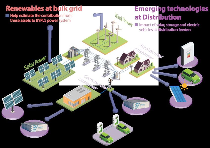
Executive Summary
Context and Problem Description
The Government of India has set a target of installing 175 GW of renewable energy capacity by the year
2022, which includes 100 GW from solar, 60 GW from wind, 10 GW from bio-power, and 5 GW from
small hydropower. Out of 100 GW solar, 40 GW is targeted from rooftop solar photovoltaics (PV). These
renewable targets can lead to a new paradigm for power grid planning and operations.

Historically, power distribution utilities were designed to serve low voltage loads within their territories,
and for decades their planning works were based on the premise that customers only consume power.
During this time, distribution utilities learned customer consumption patterns, identified peak, off-peak,
and shoulder hours and crafted proficient planning and operational strategies to match them.

Over the past decade, solar PV and wind energy adoption has increased at all scales (transmission and
distribution), as illustrated in Figure ES-1. Also, recent and anticipated adoption of battery energy storage
systems (BESS) and electric vehicles (EVs) are changing the landscape of supply and demand. Some of
these emerging technologies are variable in nature and others are not fully understood, thus posing a need
for distribution utilities to update the way that they plan and operate their systems.

Opportunities and challenges posed by these technologies (solar PV, BESS and EVs) on the power
distribution grid are yet to be comprehended, holistically. Typically, wind farms are planned and built at
large scale (100 MW to GW) and interconnected to transmission systems. Solar PV, on the other hand,
can either be connected to transmission systems at the GW scale or at rooftops at the kW scale. Thus,
challenges and opportunities vary significantly depending on the size and point of interconnection
(transmission or distribution system).

 Figure ES-1. Variable renewable resources integrated on the power grid at transmission and
 distribution levels are posing challenges for distribution utilities
The research collaboration between the U.S. Agency for International Development (USAID), NREL and
BSES Yamuna Power Ltd. (BYPL) focuses on the challenges caused by renewable integration into the

www.nrel.gov/usaid-partnership vi

power grid at large. Because the challenges and opportunities vary depending on the point of
interconnection (distribution or transmission), we identified two tracks for research as listed below:

 1. Power procurement: This research track examines the challenges and opportunities caused by
 GW-scale renewable integration at the transmission level. Specifically, this track investigates the
 contribution that utility-scale renewable energy procurement provides to distribution utilities,
 both from energy and capacity perspectives. In this track of research, utility customers are only
 considered as traditional (one-directional) consumers of energy.
 2. Distributed energy resources (DERs): This research track focuses on the challenges and
 opportunities caused by many small-scale distributed renewable resource integrations at the
 distribution systems. At the power-distribution level, distribution utilities may face not only new
 solar energy technologies, but also battery energy storage and electric vehicles (EVs). Combined,
 these three technologies (solar PV, battery energy storage, and EVs) pose unique challenges to
 distribution utilities. This track focuses on assessing the net-load evolution that distribution
 utilities will observe as these emerging technologies make their way to the grid.
Power Procurement Track
As developers plan and build utility-scale solar PV and wind farms, distribution utilities sign up to
purchase power in part or full via power purchase agreements. Renewable resources, however, are
naturally variable and not completely predictable. Distribution utilities must still serve their customers’
load at all hours, so as wind and solar PV plants start to make up a significant portion of the utility’s
portfolio, the non-dispatchable resources may pose reliability challenges.

 Figure ES-2. Capacity credit of resources in traditional vs. high VG power systems 1

1
 “Gas CC” refers to combined cycle natural gas plants. The height of the blocks is not to scale and is not meant to
represent the capacity mix of any specific power system.

www.nrel.gov/usaid-partnership vii

This track considers renewable integration at bulk grids and assesses their value addition. In order for
distribution utilities such as BYPL to make informed decisions when signing power purchase agreements
(PPAs), it is crucial for them to understand how much energy and capacity their contracted renewable
energy generators can provide. We address the situation faced by utilities by modeling variable renewable
energy (VRE) plants from two perspectives: (1) energy production, and (2) capacity credit.

Capacity credit describes the percentage of a plant’s nameplate capacity that can be reliably counted on to
serve load. The capacity credit perspective is illustrated in Figure ES-2, which shows that effective
planning includes the possible contributions of VRE. Use of capacity credit unlocks a unique path for
understanding the planning reserves provided by solar PV and wind resources. To demonstrate the value
from this research, NREL utilized existing knowledge of load, VRE contracts, and planning reserves. The
framework we describe in this paper can be used by any distribution utility to assess the potential of
contracted variable renewable resources to provide accurate planning reserves.

Key Outcomes

Renewable energy will play a pivotal role in the future of Indian distribution utilities like BYPL. BYPL
has recently contracted around 250 MW of wind and 300 MW of solar PV plants across the country, some
of which have recently been commissioned. However, due to the variable and uncontrollable nature of
these weather-based generation, adding such resources to a utility’s portfolio is more complicated than
adding traditional fuel-based resources. To set up an efficient power purchase agreement with an RE
generator, for instance, a utility needs to understand the potential of the plant to both produce energy and
provide capacity when it is most needed.

The goal of this research track is to understand the full value of these specific generation resources to the
energy and capacity needs of BYPL. As wind and solar PV plants start to make up a significant portion of
BYPL’s portfolio, understanding the full value of VREs becomes critical to avoiding overinvesting in
generation capacity. NREL developed a reusable framework that can be deployed as new wind and solar
plants are considered for future generation needs and has applied it to the recent 550 MW of contracted
VRE capacity.

The key outcomes from the study are listed below. Because BYPL has distinct winter and summer
consumption patterns, the findings are broken up into these seasons.

 1. Capacity factor for all additional utility-scale renewable energy is estimated to be 27% in
 summer (March to October) and 15% in winter (November to January). In 2019, BYPL
 served 7,314 MWh of load. Had all the additional 250 MW wind, and 300 MW solar plants been
 commissioned in 2019, BYPL’s system would have experienced 15.2% annual renewable
 penetration by generation, and 16.0% and 15.2% renewable penetration in summer and winter,
 respectively.

 2. Wind energy, especially when imported from Coimbatore, Tamil Nadu, can contribute
 significantly to BYPL’s planning reserve. Solar PV supplies minimal benefit to the planning
 reserve. The wind plants modeled in this study have a capacity credit of 53%. This means that
 53% of the planned installed wind capacity can be relied upon during periods of high system risk.
 The Coimbatore plant has a capacity credit of 64%, and aggregate VRE has a capacity credit of
 29%. These values are quite high compared to other service regions. For instance, the Southwest
 Power Pool, which contains some of North America’s strongest and most consistent wind
 resources, measured its wind capacity credit at 24.3%. But previous studies show that the

www.nrel.gov/usaid-partnership viii

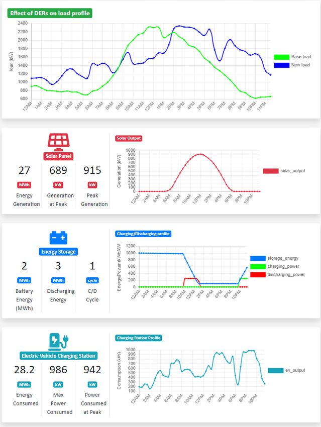
capacity credit of wind and solar PV often reduces dramatically as these resources make up a
 larger percentage of the generation mix (Haley 2019).

 3. Wind turbine model and hub height have a significant impact on estimated output and
 capacity credit. Understanding the physical attributes of the contracted wind is critical for
 efficient system-wide planning. For example, modeling the wind turbines with a 110-meter rotor
 diameter mounted at a 110-meter hub height resulted in an annual energy production 72% higher
 than that measured with turbines with an 80-meter rotor diameter mounted at 80 meters.
 Furthermore, performing the capacity credit analysis with a 110-meter rotor diameter mounted at
 110 meters resulted in a 68% capacity credit, whereas analyzing 80-meter rotor diameter turbines
 mounted at 80 meters produced an approximate capacity credit of 45%. This equates to a 57-MW
 change in firm capacity needed to fill the gap in the capacity planning reserve margin for BYPL.
 As this difference is greater than the nameplate capacity of one of the wind plants, identifying
 these parameters is necessary for producing precise results in future analyses.

 4. As renewable energy penetration increases in BYPL’s system, the capacity credit of VRE
 plants may decline. While wind capacity credit in our study remains relatively stable at high
 penetrations, solar PV capacity credit drops to zero after 15% VRE penetration. This finding,
 however, does not take into account the benefit of increased geographic diversity that will likely
 arise from increased penetration.

DER Track
Focusing on several smaller size installations (also referred to as distributed assets), this track looks at the
impact of emerging technologies on customer load shape and their aggregated form (i.e., distribution
feeder profile). Grid-connected DERs—such as solar PV, BESS, and EVs—are expected to increase
substantially in distribution systems in the coming years. These emerging technologies pose challenges to
distribution utilities, forcing overhauls in infrastructure planning and operational practices. They can also
cause more frequent system operational violations (e.g., network voltage bounds and loading thresholds)
if not properly integrated; however, if well understood and managed, DERs can also create opportunities
for distribution utilities such as increased demand, flexible loads, and flatter load curves.

 Figure ES-3. Illustration of modules in the EVOLVE interactive dashboard developed by NREL
The impacts on the localized power distribution grid from these emerging technologies manifest in
possible increased infrastructure investments and erratic shifts in demand patterns. These impacts are not
yet well understood, and analytical solutions are not readily available. To address these challenges, NREL

www.nrel.gov/usaid-partnership ix

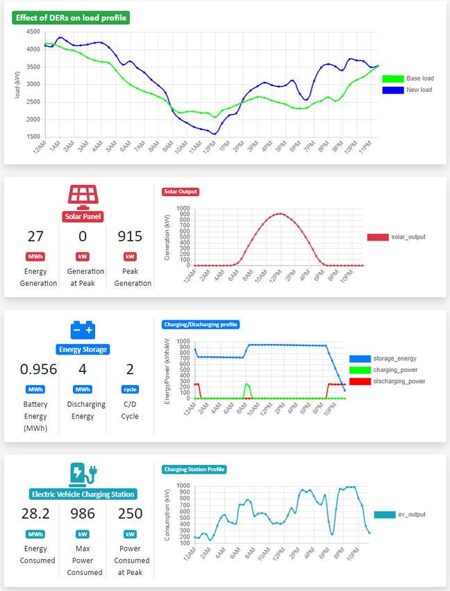
developed a scalable framework in the form of an interactive dashboard, EVOLVE (EVOlution of net-
Load Variation from Emerging technologies). EVOLVE represents a set of models/algorithms developed
by NREL that can help a distribution utility understand the potential impacts of having more DERs and
emerging technologies to a feeder. Using this interactive dashboard distribution utilities can assess
relevant scenarios (e.g., increased penetration of rooftop PV on a feeder), observe the predicted shift in
customer demand, and make decisions accordingly. EVOLVE has key modules that enable utilities to
transform existing data to usable information. The modules are load disaggregation, EVs, and BESS
integration. Tunable parameters include integration levels of solar PV, EV, and BESS, as illustrated in
Figure ES-3.

Key Outcomes

The DERs research track was set up to help BYPL understand the evolution of customer demand with the
growing adoption of emerging technologies. As illustrated in Figure ES-4, customer demand evolves
incrementally as these DERs get integrated. Typical observations include: (1) solar PV integration creates
a dip during the afternoons; (2) EVs add to the base load during night; and (3) energy storages reduce
early morning peaks. All these incremental updates happening at scale in distribution utilities quickly
escalate to a unique shift in consumption at distribution transformers. Aggregated demand shift at
distribution transformers leads to a distinct change at the distribution feeder head.

 Figure ES-4. Illustration of evolving customer demand as emerging technologies are integrated
 with the distribution grid
The distributed technologies at customers’ premises create small shifts in demand that, when aggregated,
intensify the need for significant overhaul in utility operation and planning. For this purpose, NREL
developed a set of comprehensive modeling tools and packaged those as a publicly available, interactive
dashboard, which any distribution utility can use to learn the aggregate impacts of customer adoption of
emerging distributed technologies. This dashboard—EVOLVE—helps distribution utilities to better
understand feeder-level impacts of adding more of these emerging technologies, such as solar PV, EVs,
and BESS. The dashboard allows for easy changes to inputs, such as penetration level of PV on a feeder,
to allow for a quick understanding of how the network may be impacted and help decision-making
regarding whether further technical studies may be required.

One of the key outcomes from DERs research is this easy-to-use open-source dashboard for learning
evolution of net load with increasing emerging technologies. The view of the EVOLVE dashboard is
shown in Figure ES-5. Figure ES-6 summarizes some analytics out of the dashboard, regarding a set of
EV integration scenarios for a given fleet of vehicles in a feeder area. This plot showcases how distributed

www.nrel.gov/usaid-partnership x

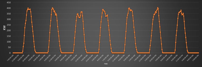
or residential charging creates overnight EV loading spikes, and more centralized approach such as EV
charging stations can spread out the load temporally.

 Figure ES-5. Partial view of dashboard for net load evolution study (EVOLVE)

 Figure ES-6. Net load profile for a charging station operation for a day

www.nrel.gov/usaid-partnership xi

Table of Contents
1 Introduction .......................................................................................................................................................... 1
 1.1 Background on the Research ......................................................................................................... 1
 1.2 Power Procurement: Estimating Capacity Credit From Utility-Scale Wind and Solar ................. 1
 1.3 DERs: Evolution of Net Load With Growing Emerging Technologies ....................................... 3
2 Power Procurement: Estimating Capacity Credit From Utility-Scale Wind and Solar ................................ 6
 2.1 Methods: Weather Resource Data ................................................................................................. 6
 2.2 Methods: Wind Modeling ............................................................................................................. 6
 2.3 Methods: Solar PV Modeling ........................................................................................................ 8
 2.4 Results: Energy Contribution ...................................................................................................... 10
 2.4.1 Results: Wind Energy Contribution ...................................................................... 10
 2.4.2 Results: Solar PV Energy Contribution ................................................................ 13
 2.5 Capacity Contribution of Renewable Energy Plants: Capacity Credit ........................................ 14
 2.5.1 Capacity Credit Method 1: Capacity Factor Approximation ................................ 16
 2.5.2 Capacity Credit Method 2: Reliability Modeling .................................................. 20
 2.6 Capacity Credit Results ............................................................................................................... 24
 2.7 Renewable Energy Penetration Scenarios ................................................................................... 25
3 DERs: Evolution of Net Load With Increasing Emerging Technologies ....................................................... 29
 3.1 Data Selection ............................................................................................................................. 29
 3.2 Down-Selection of Distribution Feeders ..................................................................................... 30
 3.3 Load Disaggregation Module ...................................................................................................... 31
 3.3.1 Model Description ................................................................................................. 31
 3.3.2 Model Outputs ....................................................................................................... 32
 3.3.3 Average Power-to-Peak-Power Ratio ................................................................... 38
 3.3.4 Percentage Peak Power Reduction ........................................................................ 39
 3.4 EV Integration Module................................................................................................................ 42
 3.4.1 Modeling Overview............................................................................................... 44
 3.4.2 Scenario Highlights ............................................................................................... 45
 3.5 BESS Sizing Algorithm .............................................................................................................. 47
 3.5.1 Peak Shaving BESS Sizing Algorithm.................................................................. 48
 3.5.2 Behind-the-Meter Applications Sizing Algorithm ................................................ 51
 3.5.3 Charging/Discharging Time and Threshold Selection Algorithm......................... 53
 3.6 Dashboard for Net Load Profile Analysis ................................................................................... 56
 3.6.1 Dashboard Overview ............................................................................................. 56
 3.6.2 Net Load Evolution Study Use Cases ................................................................... 58
 3.7 Use-Case Analyses on Selected Distribution Feeders ................................................................. 63
4 Conclusions ......................................................................................................................................................... 67

www.nrel.gov/usaid-partnership xii

List of Figures
Figure ES-1. Variable renewable resources integrated on the power grid at transmission and distribution
levels are posing challenges for distribution utilities ................................................................................... vi
Figure ES-2. Capacity credit of resources in traditional vs. high VG power systems ................................ vii
Figure ES-3. Illustration of modules in the EVOLVE interactive dashboard developed by NREL ............ ix
Figure ES-4. Illustration of evolving customer demand as emerging technologies are integrated with the
distribution grid............................................................................................................................................. x
Figure ES-5. Partial view of dashboard for net load evolution study (EVOLVE)....................................... xi
Figure ES-6. Net load profile for a charging station operation for a day..................................................... xi
Figure 1. Average daily load profiles for 2014–2019, plotted for summer (left) and winter (right). ........... 3
Figure 2. Illustration of evolving customer demand as emerging technologies get integrated with the
distribution grid............................................................................................................................................. 4
Figure 3. Process involved in developing EVOLVE for assessing evolution of net load with growing
emerging technologies .................................................................................................................................. 5
Figure 4. Power curves for a 2-MW turbine model with 80-meter rotor diameter (V80-2.0) mounted at an
80-meter hub height (left), and a 2-MW turbine model with 110-meter rotor diameter (V120-2.0) mounted
at a 110-meter hub height (right). ................................................................................................................. 8
Figure 5. Wind power output for November through February. The wind resource is light and variable,
rarely surpassing a 60% capacity factor...................................................................................................... 11
Figure 6. Heat map showing impact of wind turbine model and hub height on annual energy production of
the three wind plants in BYPL’s portfolio. ................................................................................................. 12
Figure 7. Comparison of summer power profiles for the two wind turbine models described in Figure 3. 13
Figure 8. Illustrative firm capacity stacks for a traditional (all thermal and hydro) and a high renewable
energy power system................................................................................................................................... 15
Figure 9. Representative capacity factor approximation results utilizing different percentages of load
hours, compared with capacity credit calculated with a more robust method. ........................................... 17
Figure 10. Time-of-day histogram of BYPL's top 10% load hours (left axis), overlaid with the annual
average wind and solar PV production (right axis)..................................................................................... 18
Figure 11. Example day, which represents the difference between demand and net load .......................... 19
Figure 12. Time-of-day histogram of BYPL's top 10% net load hours (left axis), overlaid with the annual
average wind and solar PV production (right axis)..................................................................................... 19
Figure 13. Time-of-day histogram of all hours in a year with a calculated LOLP > 1% (left axis), overlaid
with the annual average wind and solar PV production (right axis). .......................................................... 20
Figure 14. The workflow for NREL's in-house resource adequacy model, PRAS ..................................... 21
Figure 15. Generic representation of ELCC calculation ............................................................................. 23
Figure 16. Renewable energy penetration PRAS scenario results for ELCC ............................................. 27
Figure 17. Percentages of customers in domestic, nondomestic, and industrial sectors for three selected
feeders ......................................................................................................................................................... 31
Figure 18. Disaggregated profiles of DT1 transformer with original profile for 2019 ............................... 33
Figure 19. Disaggregated profiles of DT1 transformer with original profile for summer week of 2019 ... 34
Figure 20. Disaggregated profiles of DT1 transformer with original profile for winter week of 2019 ...... 34
Figure 21. Plot of residuals for DT1 ........................................................................................................... 35
Figure 22. Disaggregated profiles of DT2 transformer with original profile for 2019 ............................... 36
Figure 23. Disaggregated profiles of DT2 transformer with original profile for summer week of 2019 ... 36
Figure 24. Disaggregated profiles of DT2 transformer with original profile for winter week of 2019 ...... 37

www.nrel.gov/usaid-partnership xiii

Figure 25. Plot of residuals for DT2 ........................................................................................................... 37
Figure 26. Monthly average power-to-peak-power ratio for three BYPL feeders from 2016 to 2020 for 0%
to 100% PV penetration level in a step of 10% .......................................................................................... 39
Figure 27. Monthly percentage peak power reduction for three BYPL feeders from 2016 to 2020 for 0%
to 100% PV penetration level in a step of 10% .......................................................................................... 40
Figure 28. Monthly percentage of energy consumption reduction for three BYPL feeders from 2016 to
2020 for 0% to 100% PV penetration level in a step of 10% ..................................................................... 41
Figure 29. Monthly maximum change in the energy consumption in a 30-minute interval for three BYPL
feeders from 2016 to 2020 for 0% to 100% PV penetration level in a step of 10% ................................... 42
Figure 30. Charging events for different types of vehicles (sampled for one week) .................................. 43
Figure 31. Types of charging stations ......................................................................................................... 44
Figure 32. Charging station model workflow ............................................................................................. 45
Figure 33. Resultant net EV load profile for all-residential charging scenario........................................... 45
Figure 34. Key parameters for charging station operation for one day....................................................... 46
Figure 35. Net load profile for charging station operation for one day ...................................................... 46
Figure 36. Net EV charging load profile for charging station operation for one day ................................. 47
Figure 37. Various overloading conditions observed for a distribution transformer rated at 990 kVA ..... 48
Figure 38. Battery sizing map for a distribution transformer...................................................................... 49
Figure 39. Distribution transformer loading in kVA .................................................................................. 50
Figure 40. A scatter plot of the overloading instances observed in 2019 ................................................... 50
Figure 41. The BESS scheduled operation, the customer load, the PV generation, the basis load, and the
resulting net load for a domestic customer ................................................................................................. 53
Figure 42. The optimal solution of the battery scheduling subproblem for the example customer ............ 53
Figure 43. Original and new load profile with battery energy profile after applying algorithm to determine
best charging/discharging hours.................................................................................................................. 55
Figure 44. Original and new load profile with battery energy profile after applying algorithm to determine
best charging/discharging thresholds (for power-based strategy) ............................................................... 56
Figure 45. Partial view of dashboard for net load evolution study (EVOLVE).......................................... 56
Figure 46. Schematic software architecture for EVOLVE ......................................................................... 57
Figure 47. Base or native load profile of summer week in a domestic distribution transformer for 2019 . 59
Figure 48. Base and new load profiles after addition of 100 kW of solar for one week in June 2019 ....... 59
Figure 49. Solar profile and metrics specific to solar energy generation for summer week of 2019 ......... 60
Figure 50. Base and net load profile with 50 EVs for summer week of 2019 ............................................ 60
Figure 51. EV power profile and metrics of energy consumption for summer week of 2019 .................... 60
Figure 52. Base and new load profile with energy storage for summer week of 2019 ............................... 61
Figure 53. Battery energy, charging/discharging power profile, and metrics for summer week of 2019... 61
Figure 54. Base and new load profile with energy storage for automatic sizing and threshold selection for
summer week of 2019 ................................................................................................................................. 62
Figure 55. Battery energy, charging/discharging power profiles, and metrics for automatic sizing and
threshold selection for summer week of 2019 ............................................................................................ 62
Figure 56. Base and new load profile after adding solar, EV, and energy storage for summer week of 2019
 .................................................................................................................................................................... 63
Figure 57. Battery energy, charging/discharging power profile after adding solar and EVs for summer
week of 2019 (automatic sizing and threshold selection turned on) ........................................................... 63
Figure 58. Impact on load profile of Feeder1 due to DERs on summer day of 2019. Starting from the top,
first figure shows new and base profile, second figure shows solar generation profile (1 MW solar

www.nrel.gov/usaid-partnership xiv

capacity), third figure shows battery energy, charging and discharging profile (1,000 MWh, 500 kW), and
last figure shows aggregated consumption pattern of EVs (10 vehicles, 25% residential)......................... 64
Figure 59. Impact on load profile of Feeder2 due to DERs on summer day of 2019. Starting from the top,
first figure shows new and base profile, second figure shows solar generation profile (1 MW solar
capacity), third figure shows battery energy, charging and discharging profile (1,000 MWh, 500 kW), and
last figure shows aggregated consumption pattern of EVs (10 vehicles, 25% residential)......................... 65
Figure 60. Impact on load profile of Feeder3 due to DERs on summer day of 2019. Starting from the top,
first figure shows new and base profile, second figure shows solar generation profile (1 MW solar
capacity), third figure shows battery energy, charging and discharging profile (1,000 MWh, 500 kW), and
last figure shows aggregated consumption pattern of EVs (10 vehicles, 25% residential)......................... 66
Figure A-1. Correlogram for wind, solar PV, and load for every hour of the year..................................... 71
Figure A-2. Seasonal correlation of wind and load..................................................................................... 72
Figure A-3. Monthly correlation of wind and load ..................................................................................... 72

List of Tables
Table 1. Summary Energy Output of the Modeled Renewable Energy Plants in GWh ............................. 10
Table 2. Summary Capacity Factor of the Modeled Renewable Energy Plants ......................................... 10
Table 3. P50/P90 solar analysis for 2010–2014. ......................................................................................... 14
Table 4. Capacity Credit Results for Each Calculation Method by Plant ................................................... 25
Table 5. Renewable Energy Penetration Scenarios..................................................................................... 26
Table 6. Results From PRAS Renewable Energy Penetration Scenarios ................................................... 27
Table 7. List of Parameters Used to Down-Select Three Distribution Feeders From the Initial Ten ......... 30
Table 8. Number of Customers in Each Customer Category for Four Distribution Transformers
 Considered in Disaggregation Model Testing........................................................................ 33
Table 9. Charger Types Considered for the Delhi Use Case ...................................................................... 44
Table 10. Optimal BESS Size and Peak Load With and Without the BESS .............................................. 52

www.nrel.gov/usaid-partnership xv

1 Introduction
India plans to deploy high levels of renewable energy on its power grid, which can greatly reduce the
carbon intensity of its economy and strengthen energy security. Compared to conventional power, India’s
renewable energy options are more variable, uncertain, and often further from demand centers.
Experience in other systems around the world has shown that when renewable energy penetration reaches
significant levels, grid operators need specialized tools to deal with the non-dispatchable and variable
nature of renewables, helping them assess the power grid’s capacity to manage challenges with electricity
reliability and affordability. Reliability issues could ultimately affect electricity end users, but are
foremost a concern for grid operators, utilities, and renewable energy investors.

BSES Yamuna Power Ltd (BYPL) is one of the five electrical utility companies operating in Delhi, India.
Growth in electrical demand has recently been accompanied by a corresponding expansion in the
penetration of solar photovoltaics (PV), both from behind the meter and as part of the wholesale
generation mix. Thus, BYPL has a vested interest in understanding two coupled features of the evolution
of its energy supply: the projected evolution of the net load profile and the potential value of procuring
utility-scale wind and solar energy to serve its loads.

1.1 Background on the Research
Distribution utilities are faced with growth in renewable energy from multiple perspectives: (1) the
growth in solar and wind at the bulk power system, affecting their power procurement strategies; and (2)
at the distribution interconnection points, affecting the traditional role of balancing supply with demand
as well as many potential technical challenges, such as maintaining system reliability and controlling
distribution component loading. The research collaboration between the National Renewable Energy
Laboratory (NREL) and BYPL takes a close look at both challenges caused by renewable integration.
Because the challenges and opportunities vary depending on the point of interconnection (distribution or
transmission), we identified two tracks for research:

 1. Power procurement research: This research track examines the challenges and opportunities
 caused by GW-scale renewable integration at the transmission level. Specifically, the track
 investigates the contribution that utility-scale renewable energy procurement provides to
 distribution utilities, both from energy and capacity perspectives. Utility customers are only
 considered as traditional consumers of energy.
 2. Distributed energy resources (DERs) research: This research track focuses on challenges and
 opportunities caused by the integration of a large number of small-scale DERs at the distribution
 systems. At the power distribution system, utilities not only manage integration of solar
 technology, but also battery energy storage and electric vehicles (EVs). Combined, these three
 technologies (solar PV, battery energy storage, and EVs) pose unique challenges to distribution
 utilities. This research focuses on assessing the net-load evolution that distribution utilities
 observe as these emerging technologies make their way to the grid.
1.2 Power Procurement: Estimating Capacity Credit from Utility-Scale
 Wind and Solar
BYPL has historically procured most of its power by contracting portions of thermal and hydropower
generators in Delhi and farther afield. As of 2019, this amounted to 1,726 MW of contracted power. The
utility does not plan to add much more thermal generation to its portfolio, and some of the thermal plants
with which they have contracts are approaching retirement. Furthermore, utility-scale wind and solar PV
have become cost-competitive with thermal generation resources, and these types of plants also help
BYPL meet its state-mandated renewable purchase obligation. As a result, the utility has contracted 250

www.nrel.gov/usaid-partnership 1

MW of wind and 300 MW of solar PV plants across the country, some of which have recently been
commissioned.

As these new wind and solar PV plants start to make up a significant portion of BYPL’s portfolio, they
will challenge the utility to reliably meet its customers’ electrical demands. The purpose of this
component of the study is to estimate the ability of these plants to do so. We address this question by
modeling each of the future variable renewable energy (VRE) plants from two perspectives: (1) energy
production, and (2) capacity credit.

Measured as a percentage of a particular generator’s nameplate capacity, capacity credit describes the
amount of power a generator can reliably provide to the system and is a critical element of power system
planning. Understanding how much capacity a renewable energy generator can reliably provide may help
inform decision making regarding PPA contracts. For instance, when planning power procurement for
future projected peak demand, assessing capacity credit may help a utility decide how much renewable
capacity of which technologies (e.g., wind, solar PV, or hybrid wind + solar PV) will contribute to
meeting its planning reserve. In addition, knowing the capacity credit of existing renewable plants will
impact how much additional capacity the utility will require from new PPAs.

There has been significant research in the capacity credit space, and many methods for its calculation
have emerged (Milligan and Porter 2005). These methods have a broad spectrum of trade-offs between
complexity and robustness. We employ two methods in this study to highlight the insights that can be
gained and the data requirements across this spectrum. First, the capacity factor approximation offers a
simple method that is easy to compute using only a spreadsheet editing tool, but it has several
shortcomings: it is deterministic, neglects thermal outages, does not accurately reflect the effects of
increasing RE penetration, and it assumes that a unit’s historical performance during high-risk hours will
continue in future years. To represent the more complex end of the spectrum we calculate effective load
carrying-capability (ELCC), which is a robust, probabilistic method used to assess system risk at every
hour. To estimate grid integration challenges in BYPL’s future, we analyze different VRE penetration
scenarios using this probabilistic method.

BYPL considers the balancing of its load and generation portfolio on a seasonal basis based on
significantly different load shapes. These are shown in Figure 1. Summer, marked by air-conditioning
loads which cause an evening peak, lasts from March to October. Winter spans November to February,
and has significantly less overall demand and two peaks, with the morning peak generally higher.
Because BYPL uses these two seasons when making procurement decisions, we split our bulk power
system results in the same fashion.

www.nrel.gov/usaid-partnership 2

Figure 1. Average daily load profiles for 2014–2019, plotted for summer (left) and winter (right).

 Note: Average wind and solar PV profiles are also plotted.

1.3 DERs: Evolution of Net Load With Growing Emerging
 Technologies
Distribution utilities had decades to master the customer consumption profiles prior to emerging
technologies (solar PV, battery energy storage systems [BESS], and EV) made its way. Historically,
power generation used to happen at specific locations, and the generated power used to flow to bulk grid
and then to distribution network, to cater to customer energy needs. Over the past decade, increased
integration of solar PV (rooftop and utility-scale) kicked off a shift in the power consumption pattern. An
aggregate effect of these solar PVs generating during the day led to the assessment of the “duck curve” as
an impact. As impact of solar PV generation on the distribution grid is being examined all around the
world, BESS and EVs are getting integrated as well.

The DERs research track was set up to help BYPL understand the evolution of customer demand with the
growing adoption of emerging technologies. As illustrated in Figure 2, customer demand evolves
incrementally as these DERs are integrated. Typical observations include: (1) solar integration creates a
dip during the afternoons; (2) EVs add the base load during night; and (3) energy storage adds load during
early mornings with reducing peaks. All these incremental updates happening at scale in the BYPL
service territory quickly escalates to a unique shift in consumption at distribution transformers.

www.nrel.gov/usaid-partnership 3

Aggregated demand shift at distribution transformers led to a distinct change at the distribution feeder
head and goes on.

 Figure 2. Illustration of evolving customer demand as emerging technologies get integrated with
 the distribution grid
These distributed emerging technologies create a small shift in demand/profile, and, when aggregated,
quickly escalate into a need for significant overhaul in utility operation and planning. For this purpose,
NREL developed an interactive dashboard—using which any distribution utility can learn the aggregate
impacts of customer adoption of distribution emerging technologies. This dashboard EVOLVE
(EVOlution of net-Load Variation from Emerging technologies), enables distribution utilities to enter
relevant scenarios, observe the shift in customer demand, and help make decisions accordingly.

EVOLVE provides a way for compiling available data in distribution utilities to evaluate the future net
load and its implications. Figure 3 illustrates the steps involved with the operation of the EVOLVE
dashboard. The first step is for users to set the desired levels of emerging technologies—PV, BESS, and
EV. The second step is to identify the duration of analysis ranging between a day to a decade. In the
second step, the user can also choose the level of aggregation, distribution transformer or feeder head.
The third step is where the user can compare the base load profile with the evolved profile and learn the
shift of the key parameters. The interactive dashboard helps distribution utilities quantify the following
parameters for desired penetration of emerging technologies in their territory:

• Customer demand along with shift in profile caused by PV and EVs
• Change in peak power at distribution transformers caused by BESS and EVs
• Variation in ramp rates caused by PV, BESS, and EVs.

www.nrel.gov/usaid-partnership 4

Figure 3. Process involved in developing EVOLVE for assessing evolution of net load with
 growing emerging technologies

www.nrel.gov/usaid-partnership 5

2 Power Procurement: Estimating Capacity Credit
 from Utility-Scale Wind and Solar
This section describes the methodologies and modeling results used to estimate the contribution of seven
new wind and solar PV plants in BYPL’s portfolio. To produce representative power profiles for the RE
plants, this study utilizes NREL’s open-source techno-economic modeling software, the System Advisor
Model (SAM) (Blair et al. 2014). SAM was designed to facilitate decision-making for project developers
as well as grid operators and planners. It can model many types of renewable energy systems, including
solar PV (small residential rooftop and large utility-scale systems), wind power (from individual turbines
and large wind farms), hybrid PV + battery systems, concentrating solar power, battery storage,
geothermal, and biomass. 2

2.1 Methods: Weather Resource Data
Wind speed and direction, and air temperature and pressure at a variety of altitudes was obtained from
data that was created for USAID’s Greening the Grid RE integration study (Palchak et al. 2016). This
data was created using the Weather Research and Forecasting model (v3.7) and is based on the 2014
weather year (Draxl et al. 2015). 3 This data set has 5-minute time interval wind resource data for 3x3 km
grid cells for all of India, and it was directly applied to sites with exact latitude and longitude information.
When the latitude and longitude of a VRE plant was not known, we used NREL’s Renewable Energy
Data Explorer to select a location with the highest-quality weather resource still within a reasonable
distance from the appropriate city or village. The RE Data Explorer is a user-friendly geospatial analysis
tool for analyzing renewable energy potential and informing decisions, specifically in developing
countries (Cox and Leisch 2019). It compiles international wind resource data into an easily
downloadable format. We used the following land-use restrictions: cropland/grassland mosaic,
cropland/woodland mosaic, deciduous broadleaf forest, dryland cropland and pasture, evergreen broadleaf
forest, evergreen needleleaf forest, herbaceous wetland, irrigated cropland and pasture, mixed forest,
mixed shrubland/grassland, mixed tundra, savanna, shrubland, snow or ice, urban and build-up land,
water bodies, wooded tundra, and wooded wetland.

To calculate detailed wind power predictions, SAM utilizes temperature, atmospheric pressure, wind
speed and direction at four altitudes: 40 m, 80 m, 100 m, and 120 m.

Solar PV modeling in SAM requires three forms of solar irradiance data, measured in W/m2: clearsky
direct horizontal irradiance, clearsky direct normal irradiance, and clearsky global horizontal irradiance.
In addition, SAM incorporates local dew point and temperature pressure in its calculations. These data
were obtained from NREL’s National Solar Radiation Database, a serially complete collection of half-
hourly time series of the above data, modeled using multichannel measurements from geostationary
satellites (Sengupta et al. 2018).
2.2 Methods: Wind Modeling
BYPL procured a total of 250 MW of utility scale wind to be commissioned by 2020. One site (100 MW)
will be located in the district of Coimbatore, Tamil Nadu, and two (50 MW each) will be portions of wind
farms in the district of Kutch, Gujarat. BYPL provided plant location and size. When the exact location

2
 SAM also incorporates financial models for various types of renewable energy developments, but the financial
implications of these VRE procurements are beyond the scope of this study.
3
 The Weather Research and Forecasting model is a product of the National Center for Atmospheric Research in
Boulder, Colorado.

www.nrel.gov/usaid-partnership 6

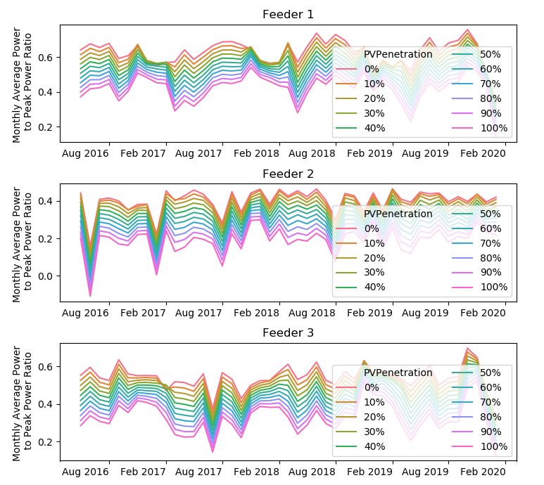
was unknown, we consulted with BYPL to identify likely locations for the site based on the quality of the
wind resource and various land use exclusions.

Few specific technical parameters were known about the wind turbines and turbine configuration to be
used in BYPL’s allocated plants. When details were uncertain, we employed the SAM defaults, which are
industry-standard assumptions:

 • Wake effects: simple wake model, turbine coefficient = 0.1, constant loss = 11.02%

 • Gridded farm configuration

 • Wake losses (internal wake + external wake + future wake) = 1.1%

 • Availability losses (turbine + balance of plant + grid) = 5.5%

 • Electrical losses (efficiency + parasitic consumption) = 2.0%

 • Turbine performance losses (suboptimal performance + generic power curve adjustment +
 site-specific power curve adjustment + high wind hysteresis) = 4.0%

 • Environmental losses (icing + environmental + degradation + exposure changes) = 2.2%.
 SAM uses a default icing loss of 0.21%. None of the wind locations experience below-
 freezing temperatures, so we use 0%.

 • Curtailment and operational strategies losses (load curtailment + grid curtailment +
 environmental and permit curtailment + operational strategies) = 2.8%

 • Wind turbine shear coefficient = 0.14.

Perhaps the most significant technical parameters used when modeling wind farm production are the size
of wind turbine rotor and hub height. Wind speeds tend to be stronger and more consistent at higher
altitudes, and larger diameter rotors capture more energy.

www.nrel.gov/usaid-partnership 7

a b

 Figure 4. Power curves for a 2-MW turbine model with 80-meter rotor diameter (V80-2.0) mounted
 at an 80-meter hub height (left), and a 2-MW turbine model with 110-meter rotor diameter (V120-
 2.0) mounted at a 110-meter hub height (right).

 Note: The blue dotted line provides a reference to compare output at 10 m/s wind speed with between the two
 models. The V110-2.0 model reaches its maximum output at slower wind speeds than the V80-2.0 turbine, and
 therefore captures more wind energy and has a higher yearly capacity factor. Adapted from NREL’s System Advisor
 Model GUI. 4

These differences are highlighted in Figure 4. Figure 4a plots the power curve (electrical output versus
wind speed) for a 2.0 MW turbine with an 80-meter rotor diameter, mounted at an 80-meter hub height.
The curve exhibits the four regions typical of all variable-speed pitch-controlled wind turbines in use
today. At just under 4 m/s, the turbine reaches its cut-in speed and begins producing electricity (Region
1). Region 2 represents the gradual ramp in power output as speeds increase. For this model turbine, 10
m/s lies in the middle of this region and corresponds to an output of about 1,100 kW, 55% of the
maximum output. Starting at 15 m/s, the turbine produces at its nameplate capacity (Region 3), until the
cut-out speed of 25 m/s when the brake is applied to prevent damage (Region 4). Region 4 is not relevant
for the wind plants studied here, as the wind resource data does not include any instances of wind speeds
surpassing 25 m/s in any of the three wind sites.

By contrast, Figure 4b shows the power curve for a 2-MW turbine with a 110-meter rotor diameter,
mounted at 110-meter hub height. While both turbines have a maximum output of 2 MW, the larger
turbine reaches this maximum at 10 m/s, two-thirds the speed of the smaller wind turbine. Furthermore,
the cut-in speed of the larger turbine is 2 m/s, so it will start producing electricity in lighter winds.

2.3 Methods: Solar PV Modeling
BYPL’s new solar PV procurements consist of four separate locations, summing to 300 MW: two 50-
MW allotments and two 100-MW allotments, grouped into two power purchase agreements. All sites are
located in the dry and relatively cloud-free state of Rajasthan. The solar resource is quite consistent across
the year in Rajasthan, though there is a dip during the cloudier monsoon season.

Using developer information, geography, and local news reports, we were able to positively identify the
locations of three of these sites. To locate the final site, a 100 MW solar PV allocation near Jodhpur, we
used the RE Data Explorer heuristic method described in Section 2.1. Candidate locations for the fourth

4
 Vestas turbines were used for reference. The figure highlights the smallest (left) and largest (right) models
available in SAM.

www.nrel.gov/usaid-partnership 8

site were abundant, but because the solar resource in Rajasthan is notably flat across a large geographic
area, the exact location would have little effect on the modeled power output.

As with wind, we largely relied on SAM’s default technical assumptions:

 • Array type = fixed open rack

 • Ground coverage ration = 0.4

 • Azimuth = 180 degrees

 • Tilt angle = latitude of the site, rounded to nearest degree

 • Inverter efficiency = 96%

 • Module type = standard silicon (thin film cadmium telluride modules for the Pokharan site)

 • Total system losses = 11.42%:

 o Soiling = 2%

 o Shading = 0% (changed from the SAM default of 3%, due to Rajasthan’s perennially
 clear skies)

 o Snow = 0%

 o Mismatch = 2%

 o Wiring = 2%

 o Connections = 0.5

 o Light-induced degradation = 1.5%

 o Nameplate = 1%

 o Age = 25 years

 o Availability = 3%.

No solar PV array will operate at its maximum nameplate capacity more than a handful of hours of the
year, if at all. Therefore, solar PV inverters are usually sized below the nameplate capacity of the solar
panel array to which they are connected. Energy is curtailed during times when the array produces more
than the inverter can handle, but the revenue lost from not converting this energy will often be made up
by the lower cost of the smaller inverter. Adjusting the ratio of solar panel nameplate capacity to inverter
capacity—known as the “DC-to-AC ratio”—allows solar PV developers to fine-tune this trade-off. For
instance, a 100-MW solar farm modeled with a DC-to-AC ratio of 1.1 will have a rated inverter size (and
maximum AC power capacity) of 91 MW. We assume a standard DC-to-AC ratio of 1.1 based on typical
PV array designs in the United States. The solar resource in Rajasthan is significantly more seasonally
and diurnally consistent than the solar resource in North America and other locations, so this is likely a
conservative estimate.

www.nrel.gov/usaid-partnership 9

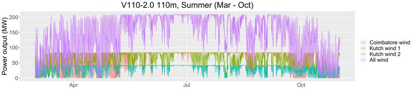
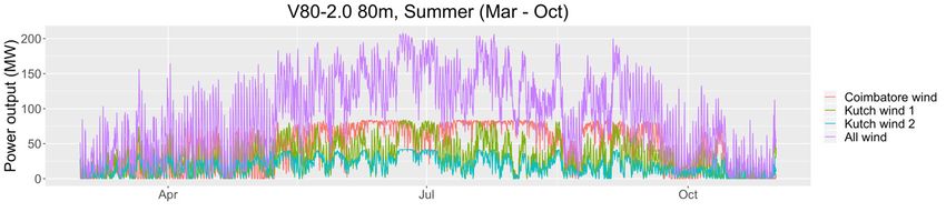
2.4 Results: Energy Contribution
Table 1 summarizes the summary energy production, in GWh, for each of the VRE plants. The capacity
factor, as a percentage, is reported in Table 2. Because the total available renewable resource varies
greatly with the season, grid operators will have to employ novel flexibility strategies.

 Table 1. Summary Energy Output of the Modeled Renewable Energy Plants, in GWh

 Coimbatore Kutch Kutch All Jaisalmer Jaisalmer Jodhpur Jodhpur All All
 Wind (100 Wind Wind Wind PV 1 (100 PV 2 (50 PV 1 PV 2 (50 Solar RE
 MW) 1 (100 2 (50 (250 MW) MW) (100 MW) PV (550
 MW) MW) MW) MW) (300 MW)
 MW)

 Summer 261 168 106 534 116 56 114 56 342 876
 (Mar–
 Oct)

 Winter 24 32 19 74 56 27 55 27 164 239
 (Nov–
 Feb)

 All Year 285 199 125 609 172 83 169 83 506 1,114

 Table 2. Summary Capacity Factor of the Modeled Renewable Energy Plants, in %

 Coimbatore Kutch Kutch All Jaisalmer Jaisalmer Jodhpur Jodhpur All All
 Wind (100 Wind Wind Wind PV 1 (100 PV 2 (50 PV 1 PV 2 (50 Solar RE
 MW) 1 (100 2 (50 (250 MW) MW (100 MW PV (550
 MW) MW) MW) solar PV) MW) solar (300 MW)
 PV) MW)

 Summer 44% 28% 36% 36% 20% 19% 19% 19% 19% 27%
 (Mar–
 Oct)

 Winter 8% 11% 13% 10% 19% 19% 19% 19% 19% 15%
 (Nov–
 Feb)

 All Year 32% 23% 28% 28% 20% 19% 19% 19% 19% 23%

2.4.1 Results: Wind Energy Contribution
Wind energy in India exhibits large seasonal variability due to starkly different wind patterns during the
center of the summer season, also referred to as the Indian Summer Monsoon. During this time, wind
capacity factors increase dramatically across the region, and so it is responsible for most of the hours of
maximum wind generation. This time also corresponds to the periods of highest load in Delhi. As such,
wind energy, in general, provides a relatively dependable resource when it is most needed. This effect,
formalized in a metric called capacity credit, is described in greater detail in Section 2.2. By contrast,
wind energy during the winter months of November through February is substantially lower. As shown in
Figure 5, the wind farms rarely surpass 60% capacity factor in this season.

www.nrel.gov/usaid-partnership 10