Prospects for Magnetography in the Chromosphere and Transition Region Thanks to: Alan Gary, Jack Harvey, Harry Jones, Bruce Lites, Jason Porter ...
←
→
Page content transcription
If your browser does not render page correctly, please read the page content below
Prospects for
            Magnetography in the Chromosphere
                  and Transition Region

Thanks to: Alan Gary, Jack Harvey, Harry Jones, Bruce
Lites, Jason Porter, Andy Skumanich, Hector Socas-
Navarro, Ted Tarbell
Short Version — Chromosphere
• Gaudy cartoons notwithstanding, we don’t understand chromospheric
structure and dynamics.
• This is an obstacle to unraveling energy transport to and from the
upper atmosphere.
• Measuring B in the chromosphere is a necessary part of a complete
picture.
• Recent progress in NLTE inversion for chromospheric lines opens up
observational opportunities.
• It will likely take 5–10 years of ground-based observation and theory
for chromospheric magnetography to become a standard tool
comparable with photospheric magnetography today …
• … but the chromosphere will always be harder.Short Version — Transition Region
• The magnetic structure of transition-temperature structures is
unquestionably central to their role in energy transport.
• The possibilities for measurement are real but limited.
• Space is the place.
• Full vector measurements are probably unrealistic.
• What are the questions that a measurement of line-of-sight flux will
answer? (Keeping in mind
• Small filling factor
• Often optically thin
• Highly dynamic)Why It Matters — Chromosphere I.
Bz at the Photosphere Potential Field B. C. Low, ApJ
399, 300 (1992)
With Both Field-Aligned and Cross-Field Currents
⇒ Force balance
Selected Low-Lying Field Lines Larger Subset of Field LinesWhy It Matters — Chromosphere II.
⇒ Connecting the Solar Atmosphere
TRACE
Cartoon Evolution (Schrijver)
Moss, carpet, canopies, fibrils,
filaments, spicules, COmosphere,
K2V bright points, …
BBSOWhy It Matters — Transition Region • Magnetic field in the hot atmosphere: at least one data point would be nice! • Genuinely β
State of the Art — Chromosphere I.

              ⇒ Large spatial scales

                • axial field in filament channels

                • unipolar, quasi-vertical connections
                between active regions

            J. Harvey
State of the Art — Chromosphere II.
⇒ Temporal Differences
K. Harvey, Jones,
Schrijver, Penn
(1999)
Figure 1. Section of the photospheric and chromospheric magnetograms showing the cancelation of
a positive polarity (white) magnetic element with a negative network (black) observed on 16 June
1998 (white circles). Note the more rapid disappearance of the positive (white) pole earlier in the
chromosphere than in the photosphere. The bottom three sets of panels show the corresponding EIT
images in He II 304 Å and TRACE images in Fe IX/X 171 Å and Fe XII 195 Å.State of the Art — Chromosphere III.
⇒ Quantitative inversion
Two magnetic components in a sunspot umbra Inversion of synthetic data (VAL-C reference)
H. Socas-Navarro et al.State of the Art — Transition Region
SMM/UVSP (Tandberg-Hanssen et al., 1981)
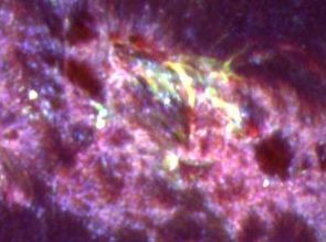
NRL VAULT Rocket, Lα, 1999
C IV, 2001Challenge — Transition Region
− v 2
I=I e = Gaussian emission profile (or emission core of a deep absorption line)
p
V = − vB cos γ ∂I / ∂v = Stokes V for weak splitting
Vmax = 0.858 I p vB cos γ = Peak magnitude of Stokes V
Q = − ( vB sin γ ) ∂ 2 I / ∂v 2 =
2
Stokes Q for weak splitting
Qmax = 0.223 I p ( vB sin γ ) 2 = Peak magnitude of Stokes Q
The C IV lines are 1548.2 Å (geff = 0.65) and 1550.8 Å (geff = 0.75).
The λ1548 line is about twice as strong as λ1550 and has an observed FWHM ≈ 200−390 mÅ
or ∆λE ≈ 120–230 mÅ.
C IV λ1548
100 G 500 G 1000 G 3000 G
∆λE=120 mÅ
Vmax/Ip 5.2e-4 0.0026 0.0052 0.016
Qmax/Ip 8.2e-8 2.0e-6 8.2e-6 7.4e-5
Qmax/Vmax 1.1e-4 5.6e-4 0.0011 0.0033Approaches — Chromosphere
Line (nm) Plus Minus
Ca II triplet (849,854,866) C-response, λ, ∆geff , λ
~ unblended,
5-level + CRD OK
Ca II H & K (393, 397) C-response RT
Mg I b 1,2, (518,517) ∆geff C-response, RT
Mg II h & K (279,280) C-response, λ RT, λ
Na D2 (590) C-response
Hα (656) C-response everything else
Hβ (486)
He I (1083) C-response weak, blended
Stokes profiles
Geometry Radiation FieldWhat Will Solar-B Do?
(in this area)
• Chromosphere
• Vector polarimetry in Mg b with the FPP tunable filter
• ~ 75 mÅ bandpass
• Low photon flux in the line core, will require long integrations
to reach good S/N (~1000:1)
• Transition Region
• Not Solar-B; need a proof-of-concept such as SUMIWhat Will Ground-Based
Telescopes Do?
• DST, THEMIS, Gregor, NSST et al.
• Create a mature technique with a recognized body of results
• Solar-C et al.
• Hanle effect measurements of prominences and filaments
• ATST
• Flux, flux, flux
• Push to high angular resolutionState of the Art — Transition Region
SMM/UVSP (Tandberg-Hanssen et al., 1981)
NRL VAULT Rocket, Lα, 1999
C IV, 2001Beyond Solar-B
• Scientific prerequisites:
• Demonstrate that chromospheric magnetography is a mature and
powerful tool.
• Sharpen the case for limited measurement of the transition plasma.
• ATST and friends
• Comprehensive TR instrument suite with polarimetry
• 2-meter class space telescope
• For angular resolution better than Solar-B but not diffraction-limitedSummary: Magnetography in the Chromosphere and Transition Region
Why?
• Unravel energy transport to and from the upper atmosphere
• Measure B where atmosphere is most nearly force-free
Key Challenge in the Chromosphere
• Interpreting polarimetry of NLTE lines formed in a three-
dimensionally inhomogeneous, dynamic atmosphere
Stokes profiles Complex Structure and Energy
Transport (Schrijver 2000)
BBSO
Hα
Radiation
Geometry
Field
VAULT Lα
(1999)
Key Challenges in the Transition Region
• Weak polarimetric signal (full vector field unrealistic)
• Isolating questions that line-of-sight flux measurements
can answer TRACE UV
How? including C IV
(1998)
• Chromosphere: large ground-based telescopes, Solar-B
• Transition region: begin with rocket proof of conceptYou can also read