Quantifying Privacy Loss of Human Mobility Graph Topology
←
→
Page content transcription
If your browser does not render page correctly, please read the page content below
Proceedings on Privacy Enhancing Technologies ; 2018 (3):5–21

Dionysis Manousakas*, Cecilia Mascolo, Alastair R. Beresford, Dennis Chan, and Nikhil Sharma

Quantifying Privacy Loss of
Human Mobility Graph Topology
Abstract: Human mobility is often represented as a
mobility network, or graph, with nodes representing
                                                                1 Introduction
places of significance which an individual visits, such
                                                                Our mobile devices collect a significant amount of data
as their home, work, places of social amenity, etc., and
                                                                about us and location data of individuals are particu-
edge weights corresponding to probability estimates of
                                                                larly privacy sensitive. Furthermore, previous work has
movements between these places. Previous research has
                                                                shown that removing direct identifiers from mobility
shown that individuals can be identified by a small num-
                                                                traces does not provide anonymity: users can easily be
ber of geolocated nodes in their mobility network, ren-
                                                                reidentified by a small number of unique locations that
dering mobility trace anonymization a hard task. In this
                                                                they visit frequently [6, 43].
paper we build on prior work and demonstrate that even
                                                                     Consequently, some approaches have been proposed
when all location and timestamp information is removed
                                                                that protect location privacy by replacing location co-
from nodes, the graph topology of an individual mobil-
                                                                ordinates with encrypted identifiers, using different en-
ity network itself is often uniquely identifying. Further,
                                                                cryption keys for each location trace in the popula-
we observe that a mobility network is often unique, even
                                                                tion. This preprocessing results in locations that are
when only a small number of the most popular nodes
                                                                strictly user-specific and cannot be cross-referenced be-
and edges are considered. We evaluate our approach us-
                                                                tween users. Examples include the research track of
ing a large dataset of cell-tower location traces from
                                                                the Nokia Mobile Data Challenge,1 where visited places
1 500 smartphone handsets with a mean duration of 430
                                                                were represented by random integers [14]; and identifi-
days. We process the data to derive the top−N places
                                                                able location information collected by the Device An-
visited by the device in the trace, and find that 93% of
                                                                alyzer dataset,2 including WiFi access point MAC ad-
traces have a unique top−10 mobility network, and all
                                                                dresses and cell tower identifiers, are mapped to a set
traces are unique when considering top−15 mobility net-
                                                                of pseudonyms defined separately for each handset [35].
works. Since mobility patterns, and therefore mobility
                                                                Moreover, temporal resolution may also be deliberately
networks for an individual, vary over time, we use graph
                                                                decreased to improve anonymization [11] since previous
kernel distance functions, to determine whether two mo-
                                                                work has demonstrated that sparsity in the temporal
bility networks, taken at different points in time, rep-
                                                                evolution of mobility can cause privacy breaches [6].
resent the same individual. We then show that our dis-
                                                                     In this paper, we examine the degree to which mo-
tance metrics, while imperfect predictors, perform sig-
                                                                bility traces without either semantically-meaningful lo-
nificantly better than a random strategy and therefore
                                                                cation labels, or fine-grained temporal information, are
our approach represents a significant loss in privacy.
                                                                identifying. To do so, we represent location data for an
Keywords:  Mobility privacy;             De-anonymization;      individual as a mobility network, where nodes corre-
k−anonymity; Graph kernels.                                     spond to abstract locations and edges to their connec-
DOI 10.1515/popets-2018-0018
                                                                tivity, i.e. the respective transitions made by an individ-
Received 2017-11-30; revised 2018-03-15; accepted 2018-03-16.   ual between locations. We then examine whether or not
                                                                these graphs reflect user-specific behavioural attributes
                                                                that could act as a fingerprint, perhaps allowing the re-
*Corresponding Author: Dionysis Manousakas:                     identification of the individual they represent. In partic-
University of Cambridge, dm754@cam.ac.uk.                       ular, we show how graph kernel distance functions [34]
Cecilia Mascolo: University of Cambridge and
                                                                can be used to assist reidentification of anonymous mo-
the Alan Turing Institute, cm542@cam.ac.uk.
Alastair R. Beresford: University of Cambridge,                 bility networks. This opens up new opportunities for
arb33@cam.ac.uk.                                                both attack and defense. For example, patterns found
Dennis Chan: University of Cambridge, dc598@cam.ac.uk.
Nikhil Sharma: University College London,
nikhil.sharma@ucl.ac.uk.                                        1 http://www.idiap.ch/project/mdc
                                                                2 https://deviceanalyzer.cl.cam.ac.uk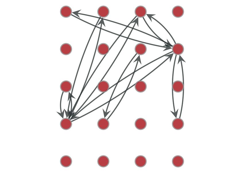
Quantifying Privacy Loss of Human Mobility Graph Topology     6

in mobility networks could be used to support auto-               a randomised mechanism using no structural infor-
mated user verification where the mobility network acts           mation contained in the mobility networks.
as a behavioural signature of the legitimate user of the
device. However the technique could also be used to link
together different user profiles which represent the same
individual.
                                                              2 Related Work
     Our approach differs from previous studies in loca-
tion data deanonymization [7, 9, 10, 21], in that we aim      2.1 Mobility Deanonymization
to quantify the breach risk in preprocessed location data
that do not disclose explicit geographic information, and     Protecting the anonymity of personal mobility is no-
where instead locations are replaced with a set of user-      toriously difficult due to sparsity [1] and hence mo-
specific pseudonyms. Moreover, we also do not assume          bility data are often vulnerable to deanonymization
specific timing information for the visits to abstract lo-    attacks [22]. Numerous studies into location privacy
cations, merely ordering.                                     have shown that even when an individual’s data are
     We evaluate the power of our approach over a large       anonymized, they continue to possess unique patterns
dataset of traces from 1 500 smartphones, where cell          that can be exploited by a malicious adversary with
tower identifiers (cids) are used for localization. Our       access to auxiliary information. Zang et al. analysed
results show that the data contains structural informa-       nationwide call-data records (CDRs) and showed that
tion which may uniquely identify users. This fact then        the N most frequently visited places, so called top−N
supports the development of techniques to efficiently         data, correlated with publicly released side information
re-identify individual mobility profiles. Conversely, our     and resulted in privacy risks, even for small values of
analysis may also support the development of techniques       N s [43]. This finding underlines the need for reductions
to cluster into larger groups with similar mobility; such     in spatial or temporal data fidelity before publication.
an approach may then be able to offer better anonymity        De Montjoye et al. quantified the unicity of human mo-
guarantees.                                                   bility on a mobile phone dataset of approximately 1.5M
     A summary of our contributions is as follows:            users with intrinsic temporal resolution of one hour and
– We show that network representations of individual          a 15-month measurement period [6]. They found that
     longitudinal mobility display distinct topology, even    four random spatio-temporal points suffice to uniquely
     for a small number of nodes corresponding to the         identify 95% of the traces. They also observe that the
     most frequently visited locations.                       uniqueness of traces decreases as a power law of spatio-
– We evaluate the sizes of identifiability sets formed        temporal granularity, stressing the hardness of achieving
     in a large population of mobile users for increas-       privacy via obfuscation of time and space information.
     ing network size. Our empirical results demonstrate           Several inference attacks on longitudinal mobility
     that all networks become quickly uniquely identifi-      are based on probabilistic models trained on individ-
     able with less than 20 locations.                        ual traces and rely on the regularity of human mobil-
– We propose kernel-based distance metrics to quan-           ity. Mulder et al. developed a re-identification technique
     tify mobility network similarity in the absence of se-   by building a Markov model for each individual in the
     mantically meaningful spatial labels or fine-grained     training set, and then using this to re-identify individu-
     temporal information.                                    als in the test set by likelihood maximisation [7]. Simi-
– Based on these distance metrics, we devise a                larly, Gambs et al. used Markov chains to model mobil-
     probabilistic retrieval mechanism to reidentify          ity traces in support of re-identification [9].
     pseudonymized mobility traces.                                Naini et al. explored the privacy impact of releas-
– We evaluate our methods over a large dataset of             ing statistics of individuals mobility traces in the form
     smartphone mobility traces. We consider an at-           of histograms, instead of their actual location informa-
     tack scenario where an adversary has access to           tion [21]. They demonstrated that even this statistical
     historical mobility networks of the population she       information suffices to successfully recover the identity
     tries to deanonymize. We show that by inform-            of individuals in datasets of few hundred people, via
     ing her retrieval mechanism with structural similar-     jointly matching labeled and unlabeled histograms of
     ity information computed via a deep shortest-path        a population. Other researchers have investigated the
     graph kernel, the adversary can achieve a median         privacy threats from information sharing on location-
     deanonymization probability 3.52 times higher than       based social networks, including the impact of location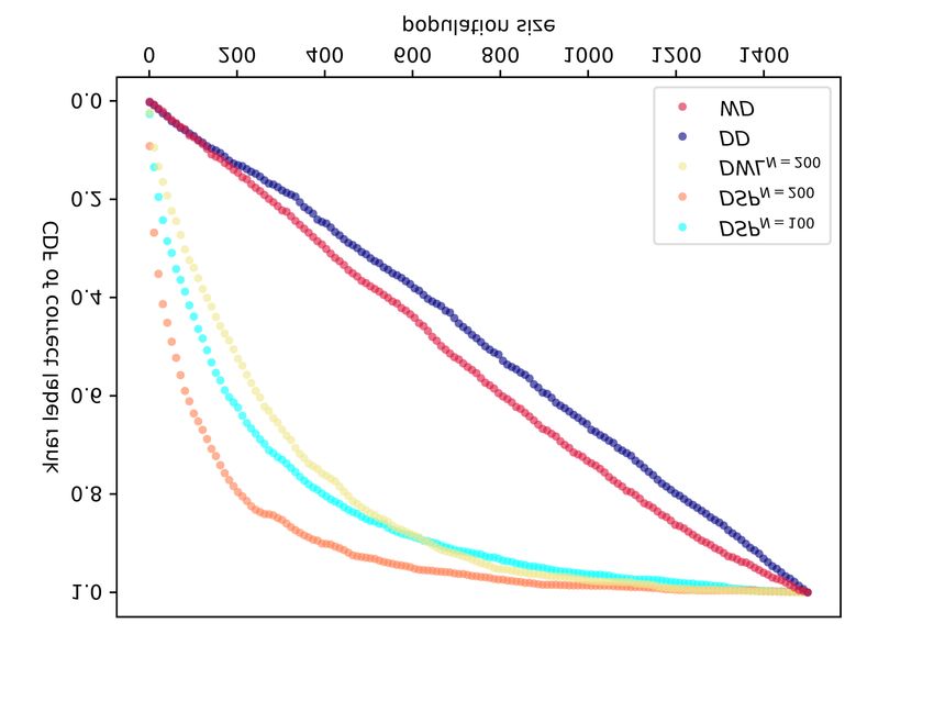
Quantifying Privacy Loss of Human Mobility Graph Topology     7

semantics on the difficulty of re-identification [27] and       reduced to a graph matching or classification problem.
location inference [2].                                         To the best of our knowledge, this is the first attempt
     All the above previous work assumes locations are          to deanonymize an individual’s structured data by ap-
expressed using a universal symbol or global identi-            plying graph similarity metrics. Since we are looking at
fier, either corresponding to (potentially obfuscated)          relational data, not microdata, standard theoretical re-
geographic coordinates, or pseudonymous stay points.            sults on microdata anonymization, such as differential
Hence, cross-referencing between individuals in the pop-        privacy [8], are not directly applicable. However, metrics
ulation is possible. This is inapplicable when location in-     related to structural similiarity, including k−anonymity,
formation is anonymised separately for each individual.         can be generalized in this framework.
Lin et al. presented a user verification method in this
setting [16]. It is based on statistical profiles of individ-
ual indoor and outdoor mobility, including cell tower ID
and WiFi access point information. In contrast, we em-
                                                                3 Proposed Methodology
ploy network representations based solely on cell tower
                                                                In this section, we first adapt the privacy framework of
ID sequences without explicit time information.
                                                                k−anonymity to the case of graph data (Section 3.1).
     Often, studies in human mobility aim to model
                                                                Next we introduce our methodology: We assume that
properties of a population, thus location data are pub-
                                                                all mobility data are initially represented as a se-
lished as aggregate statistics computed over the loca-
                                                                quence of pseudonymous locations. We also assume
tions of individuals. This has traditionally been con-
                                                                the pseudonymisation process is distinct per user, and
sidered a secure way to obfuscate the sensitive infor-
                                                                therefore locations cannot be compared between indi-
mation contained in individual location data, especially
                                                                viduals. In other words, it is not possible to determine
when released aggregates conform to k−anonymity [32]
                                                                whether pseudonymous location lu for user u is the same
principles. However, recent results have questioned this
                                                                as (or different from) location lv for user v. We convert
assumption. Xu et al. recovered movement trajecto-
                                                                a location sequence for each user into a mobility net-
ries of individuals with accuracy levels of between 73%
                                                                work (Section 3.2). We then extract feature representa-
and 91% from aggregate location information computed
                                                                tions of these networks and embed them into a vector
from cellular location information involving 100 000
                                                                space. Finally, in the vector space, we can define pair-
users [38]. Similarly, Pyrgelis et al. performed a set of
                                                                wise distances between the network embeddings (Sec-
inference attacks on aggregate location time-series data
                                                                tion 3.3) and use them in a deanonymization scenario
and detected serious privacy loss, even when individual
                                                                (Section 3.4).
data are perturbed by differential privacy mechanisms
                                                                     Our methodology is, in principle, applicable to
before aggregation [26].
                                                                many other categories of recurrent behavioural trajecto-
                                                                ries that can be abstracted as graphs, such web brows-
                                                                ing sessions [24, 42] or smartphone application usage
2.2 Anonymity of Graph Data
                                                                sequences [37]. We leave such analysis as future work.

Most of the aforementioned data can be represented as
microdata with rows of fixed dimensionality in a table.
                                                                3.1 k−anonymity on Graphs
Microdata can thus be embedded into a vector space. In
other applications, datapoints are relational and can be
                                                                Anonymity among networks refers to topological (or
naturally represented as graphs. Measuring the similar-
                                                                structural) equivalence. In our analysis we adopt the
ity of such data is significantly more challenging, since
                                                                privacy framework of k−anonymity [32] which we sum-
there is no definitive method. Deanonymization attacks
                                                                marize as follows:
on graphs have mostly been studied in the context of so-
cial networks and aimed to either align nodes between           Definition 3.1. (k−anonymity) A microdata release
an auxiliary and an unknown targeted graph [23, 29], or         of statistics containing separate entries for a number of
quantify the leakage of private information of a graph          individuals in the population satisfies the k−anonymity
node via its neighbors [44].                                    property if the information for each individual contained
     In the problem studied here, each individual’s in-         in the release is indistinguishable from at least k − 1
formation is an entire graph, rather than a node in a
graph or a node attribute, and thus deanonymization is
Quantifying Privacy Loss of Human Mobility Graph Topology 8
other individuals whose information also appears in the poral correlation among their states. In the case of mo-
release. bility data, this means that the transition by an indi-
vidual to the next location in the mobility network can
Therefore we interpret k−anonymity in this paper be accurately modelled by considering only their cur-
to mean that the mobility network of an individ- rent location. For example, the probability that an in-
ual in a population should be identical to the mobil- dividual visits the shops or work next depends only on
ity network of at least k − 1 other individuals. Re- where they are located now, and a more detailed past
cent work casts doubt on the protection guarantees of- history of places recently visited does not offer signifi-
fered by k−anonymity in location privacy [31], moti- cant improvements to the model. The alternative is that
vating the definition of l−diversity [17] and t−closeness a sequences of the states are better modelled by higher-
[15]. Although k−anonymity may be insufficient to en- order Markov chains, namely that transitions depend
sure privacy in the presence of adversarial knowledge, on the current state and one or more previously visited
k−anonymity is a good metric to use to measure the states. For example, the probability that an individual
uniqueness of an individual in the data. Moreover, this visits the shops or work next depends not only on where
framework is straightforwardly generalizable to the case they are now, but where they were earlier in the day or
of graph data. week. If higher-order Markov chains are required, we
Structural equivalence in the space of graphs corre- should assume a larger state-space and use these states
sponds to isomorphism and, based on this, we can define as the nodes of our individual mobility networks. Re-
k−anonymity on unweighted graphs as follows: cently proposed methods on optimal order selection of
sequential data [28, 39] can be directly applied at this
Definition 3.2. (Graph Isomorphism) Two graphs step.
G = (V, E) and G0 = (V 0 , E 0 ) are isomorphic (or be- Let us assume a mobility dataset from a population
long to the same isomorphism class) if there exists a of users u ∈ U . We introduce two network representa-
bijective mapping g : V → V 0 such that (vi , vj ) ∈ E iff tions of user’s mobility.
g(vi ), g(vj ) ∈ E 0 .
Definition 3.6. (State Connectivity Network): A
Definition 3.3. (Graph k−anonymity) Graph state connectivity network for u is an unweighted di-
k−anonymity is the minimum cardinality of isomor-
rected graph C u = V u , E u . Nodes vi ∈ V u correspond
phism classes within a population of graphs. to states visited by the user throughout the observation
period. An edge eij = viu , vju ∈ E u represents the in-
After clustering our population of graphs into isomor-
formation that u had at least one recorded transition
phism classes, we can also define the identifiability set
from viu to vju .
and anonymity size [25] as follows:
Definition 3.7. (Mobility Network): A mobility
Definition 3.4. (Identifiability Set) Identifiability
network for u is a weighted and directed graph Gu =
set is the percentage of the population which is uniquely
V u , E u , W u ∈ G, with the same topology as the state
identified given their top−N network.
connectivity network and additionally an edge weight
function W u : E u → R+ . The weight function assigns a
Definition 3.5. (Anonymity Size) The anonymity u to each edge eu , which corresponds to the
frequency wij ij
size of a network within a population is the cardinality
number of transitions from viu to vju recorded through-
of the isomorphism class to which the network belongs.
out the observation period.
To facilitate comparisons of frequencies across networks
3.2 Mobility Information Networks
of different sizes in our experiments, we normalize edge
weights on each mobility network to sum to 1.
To study the topological patterns of mobility, we repre-
In first-order networks, nodes correspond to distinct
sent user movements by a mobility network. A prelimi-
places the user visits. Given a high-frequency, times-
nary step is to check whether a first-order network is a
tamped, sequence of location events for a user, dis-
reasonable representation of movement data, or whether
tinct places can be extracted as small geographic regions
a higher-order network is required.
where a user stays longer than a defined time interval,
First-order network representations of mobility
using existing clustering algorithms [13]. Nodes in the
traces are built on the assumption of a first-order tem-Quantifying Privacy Loss of Human Mobility Graph Topology 9
mobility network have no geographic or timing informa- remain unchanged under structure-preserving bijection
tion associated with them. Nodes may have attributes of the vertex set, all examined graph kernels are in-
attached to them reflecting additional side information. variant under isomorphism. We briefly introduce these
For example, in this paper we consider whether attach- kernels in the remainder of the section.
ing the frequency of visits a user makes to a specific
node aids an attacker attempting to deanonymize the
user. 3.3.1 Kernels on degree distribution
In some of our experiments, we prune the mobility
networks of users by reducing the size of the mobility The degree distribution of nodes in the graph can be
network to the N most frequent places and rearranging used to quantify the similarity between two graphs. For
the edges in the network accordingly. We refer to these example, we can use a histogram of weighted or un-
networks as top−N mobility networks. weighted node degree as a feature vector. We can then
compute the pairwise distance of two graphs by taking
either the inner product of the feature vectors or passing
3.3 Graph Similarity Metrics them through a Gaussian radial basis function (RBF)
kernel:
It is not possible to apply a graph isomorphism test to
||φ(G) − φ(G0 )||2
0
two mobility networks to determine if they represent the K(G, G ) = exp − .
2σ 2
same underlying user because a user’s mobility network
is likely to vary over time. Therefore we need distance Here, the parameters of the kernel are the variance σ
functions that can measure the degree of similarity be- (in case RBF is used) and the number of bins in the
tween two graphs. Distance functions decompose the histogram.
graph into feature vectors (smaller substructures and
pattern counts), or histograms of graph statistics, and
express similarity as the distance between those feature 3.3.2 Kernel on graph atomic substructures
representations. In the following, we introduce the no-
tion of graph kernels and describe the graph similarity Kernels can use counts on substructures, such as sub-
metrics used later in our experiments. tree patterns, shortest paths, walks or limited-size sub-
We wish to compute the similarity between two graphs. This family of kernels are called R−convolution
graphs G, G0 ∈ G. Kernel functions [34], or kernels, graph kernels [12]. In this way, graphs are represented
are symmetric positive semidefinite functions, where as vectors with elements corresponding to the frequency
K(G, G0 ) : G × G → R+ , meaning that for all of each such substructure over the graph. Hence, if
n > 1, G1 , ..., Gn ∈ G, and c1 , ..., cn ∈ R, we have s1 , s2 , ... ∈ S are the substructures of interest and
Pn
# si ∈ G the counts of si in graph G, we get as feature
i,j=1 ci cj K(Gi , Gj ) ≥ 0. Each kernel function cor-
responds to some feature map φ(G), where the kernel map vectors
function can be expressed as the inner product between
φ(G) = [# s1 ∈ G , # s2 ∈ G , ...]T
feature maps, i.e., K(G, G0 ) = φ(G), φ(G0 ) . (2)
In order to ensure the result from the kernel lies with dimension |S| and kernel
in the range from −1 to 1 inclusive, we apply cosine
X
normalization as follows: K(G, G0 ) = # s ∈ G # s ∈ G0 .
(3)
φ(G0 ) s∈S
φ(G)
K(G, G0 ) = , . (1) In the following, we briefly present some kernels in
||φ(G)|| ||φ(G0 )||
this category and explain how they are adapted in our
One interpretation of this function is as the cosine sim- experiments.
ilarity of the graphs in the feature space defined by the
map of the kernel. Shortest-Path Kernel
In our experiments we apply a number of scalable The Shortest-Path (SP) graph kernel [5] expresses
kernel functions on our mobility datasets and assess the similarity between two graphs by counting the co-
their suitability for deanonymization applications on occuring shortest paths in the graphs. It can be written
mobility networks. We note in advance that as the de- in the form of equation (3) where each element si ∈ S
gree distribution and all substructure counts of a graph is a triplet aistart , aiend , n , where n is the length of theQuantifying Privacy Loss of Human Mobility Graph Topology 10
1, 3 4 3, 233 7
3 2 2 3
3, 233 2, 33 2, 33 3, 233
3 3 3, 1133 3, 1233
2, 33 5 3, 1133 8
3 3 3, 233 3, 133
1 1 1, 3 1, 3
1 1 1, 3 1, 3
3, 133 6 3, 1233 9
(a) G (b) G0 (c) G with multiset node (d) with multiset G0 (e) Label Compression
attributes node attributes
7 5 5 7
features 1 2 3 4 5 6 7 8 9
8 9
7 6
φ1 (G) = [2, 1, 3, 2, 1, 0, 2, 1, 0 ]
4 4
4 4 φ1 (G0 ) = [2, 1, 3, 2, 1, 1, 1, 0, 1 ]
(f) G relabeled (g) G0 relabeled (h) extracted feature vectors
Fig. 1. Computation of the Weisfeiler-Lehman subtree kernel of height h = 1 for two attributed graphs.
path and aistart , aiend the attributes of the starting and of atomic substructures in the kernel computation [41].
ending nodes. The shortest path set is computable in Hence, these kernels can quantify similar substructure
polynomial time using, for example, the Floyd-Warshall co-occurence, offering more robust feature representa-
algorithm, with complexity O(|V |4 ), where |V | is num- tions. DKs are based on computing the following inner
ber of nodes in the network. product:
T
K(G, G0 ) = φ G M φ G0 ,
Weisfeiler-Lehman Subtree Kernel
Shervashidze et al. proposed an efficient where φ is the feature mapping of a classical R-
method [30] to construct a graph kernel utilizing the convolution graph kernel.
Weisfeiler-Lehman (WL) test of isomorphism [36]. The In the above, M : |V|×|V| is a positive-definitive ma-
idea of the WL kernel is to measure co-occurences of trix encoding the relationships between the atomic sub-
subtree patterns across node attributed graphs. structures and V is the vocabulary of the observed sub-
Computation progresses over iterations as follows: structures in the dataset. Here, M can be defined using
1. each node attribute is augmented with a multiset of the edit distance of the substructures, i.e. the number
attributes from adjacent nodes; of elementary operations to transform one substructure
2. each node attribute is then compressed into a single to another; or M can be learnt from the data, applying
attribute label for the next iteration; and relevant neural language modeling methods [19].
3. the above steps are repeated until a specified thresh-
old h is reached.
3.4 Deanonymization of User Mobility
An example is shown in Figure 1. Networks and Privacy Leakage
If G and G0 are the two graphs, the WL subtree Evaluation
kernel is defined as follows:
3.4.1 Hypothesis
h 0 0
KW L (G, G ) = φh (G), φh (G ) ,
The basic premise of our deanonymization approach can
where φh (G) and φh (G0 ) are the vectors of labels ex-
be postulated as follows:
tracted after running h steps of the computation (Fig-
The mobility of a person across different time pe-
ure 1h). They consist of h blocks, where the i−th com-
riods is stochastic, but largely recurrent and stationary,
ponent of the j−th block corresponds to the frequency
and its expression at the level of the individual mobility
of label i at the j−th iteration of the computation. The
network is discriminative enough to reduce a person’s
computational complexity of the kernel scales linearly
privacy within a population.
with the number of edges |E| and the length h of the
For example, the daily commute to work corre-
WL graph sequence.
sponds to a relatively stable sequence of cell tow-
Deep Graph Kernels ers. This can be expressed in the mobility network of
Deep graph kernels (DK s) are a unified framework the user as a persistent subgraph and forms a char-
that takes into account similarity relations at the level acteristic behavioural pattern that can be exploitedQuantifying Privacy Loss of Human Mobility Graph Topology 11
that a training and test mobility network belonging to
the same person have common or similar connectivity
patterns, thus a high degree of similarity.
The intention of an adversary is to deanonymize a
given test network G0 ∈ Gtest , by appropriately defining
a vector of probabilities over the possible identities in
L.
(a) user 1: first half of the ob- (b) user 1: second half of the An uninformed adversary has no information
servation period observation period about the networks of the population and in the ab-
sence of any other side knowledge, the prior belief of
the adversary about the identity of G0 is a uniform dis-
tribution over all possible identities:
P lG0 = lGi = 1/|L|, for every Gi ∈ Gtraining . (4)
An informed adversary has access to the popula-
tion of training networks and can compute the pairwise
(c) user 2: first half of the ob- (d) user 2: second half of the similarities of G0 with each Gi ∈ Gtraining using a ker-
servation period observation period
nel function K. Hence the adversary can update her
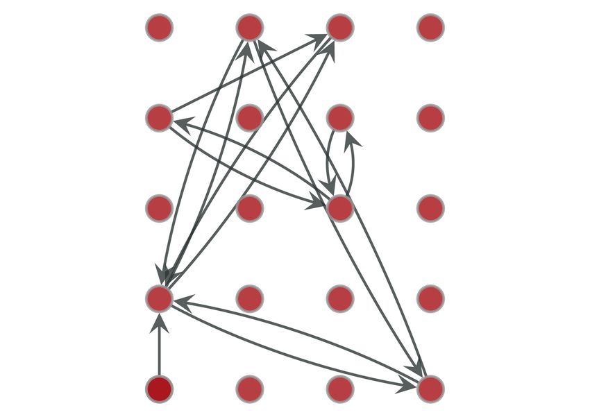
Fig. 2. Top−20 networks for two random users from the Device belief for the possible identities in L according to the
Analyzer dataset. Depicted edges correspond to the 10% most values of K. Therefore, when the adversary attempts to
frequent transitions in the respective observation window. The deanonymize identities in the data, she assigns probabil-
networks show a high degree of similarity between the mobility ities that follow a non-decreasing function of the com-
profiles of the same user over the two observation periods. More-
puted pairwise similarity of each label. Denoting this
over, the presence of single directed edges in the profile of user 2
forms a discriminative pattern that allows us to distinguish user 2 function by f , we can write the updated adversarial
from user 1. probability estimate for each identity as follows:
f K(Gi , G0 )
for deanonymization of mobility traces. Empirical ev- P lG0 = lGi |Gtraining , K = X ,
idence for our hypothesis is shown in Figure 2. For ease f K(Gj , G0 )
(5)
of presentation, in the figure, nodes between the dis- j∈L
parate observation periods of the users can be cross- for every Gi ∈ Gtraining .
referenced. We assume that cross-referencing is not pos-
sible in our attack scenario, as locations are indepen-
dently pseudonymized. 3.4.3 Privacy Loss
In the case of the uninformed adversary, the true label
3.4.2 Threat Model for any user is expected to have rank |L|/2. Under this
policy, the amount of privacy for each user is propor-
We assume an adversary has access to a set of mobility tional to the size of the population.
networks G ∈ Gtraining with disclosed identities (or la- In the case of the informed adversary, knowledge
bels) lG ∈ L and a set of mobility networks G0 ∈ Gtest of Gtraining and the use of K will induce some positive
with undisclosed identities lG0 ∈ L.3 privacy loss which will result in the expected rank of
We define a normalised similarity metric among the user to be smaller than |L|/2. The privacy loss can be
networks K : Gtraining × Gtest → R+ . We hypothesize quantified as follows:
0
P lG0 = lG0true |Gtraining , K
3 Generally we can think of lG0 ∈ J ⊃ L and assign some P L G ; Gtraining , K = −1
fixed probability mass to the labels lG0 ∈ J \ L. However, here P lG0 = lG0true
we make the closed world assumption that the training and test (6)
networks come from the same population. We make this assump-
tion for two reasons: first, it is a common assumption in works
A privacy loss equal to zero reflects no information
on deanonymization and, second, we cannot directly update our gain compared to an uninformed adversary with no ac-
beliefs on lG0 ∈ J \ L by observing samples from L. cess to graphs with disclosed identities.Quantifying Privacy Loss of Human Mobility Graph Topology 12
Let us assume that the users of our population gen- connectivity. For privacy purposes, released cid infor-
erate distinct mobility networks. As will be supported mation is given a unqiue pseudonym separately for each
with empirical evidence in the next section, this is of- user and contains no geographic, or semantic, informa-
ten the case in real-world cid datasets of few thousand tion concerning the location of users. Thus we cannot
users even for small networks sizes (e.g. for top−20 net- determine geographic proximity between the nodes and
works in our dataset). Under the above premise, the the location data of two users cannot be directly aligned.
maximal privacy loss occurs when the presented test For our experiments, we analysed cid information
network is an identical copy of a training network of collected from 1 500 handsets with the largest recorded
the same user which exists in the data of the adversary, location datapoints in the dataset. Figure 4a shows the
i.e. G0 ∈ Gtraining . This corresponds to a user determin- observation period for these handsets; note that the
istically repeating her mobility patterns over the ob- mean is greater than one year but there is lot of variance
servation period recorded in the test network. In such across the population. We selected these 1 500 handsets
a scenario, we could think that isomorphism tests are in order to examine the re-identifiability of devices with
the most natural way to compute similarity; however, rich longitudinal mobility profiles. This allowed us to
isomorphism tests will be useless in real-world scenar- study the various attributes of individual mobility af-
ios, since the stochastic nature and noise inherent in fecting privacy in detail. As mentioned in the previous
the mobility networks of a user would make them non- section, the cost of computing the adversarial posterior
isomorphic. Maximal privacy loss reflects the discrim- probability for the deanonymization of a given unlabeled
inative ability of the kernel and cannot be exceeded network scales linearly with the population size.
in real-world datasets, where the test networks are ex-
pected to be noisy copies of the training networks exist-
ing in our system. The step of comparing with the set 4.2 Mobility Networks Construction
of training networks adds computational complexity of
O(|Gtraining |) to the similarity metric cost. We began by selecting the optimal order of the network
Moreover, our framework can naturally facilitate in- representations derived from the mobility trajectories
corporating new data to our beliefs when multiple ex- of the 1 500 handsets selected from the Device Analyzer
amples per individual exist in the training dataset. For dataset. We first parsed the cid sequences from the mo-
example, when multiple instances of mobility networks bility trajectories into mobility networks. In order to
per user are available, we can use k−nearest neighbors remove cids associated with movement, we only defined
techniques in the comparison of distances with the test nodes for cids which were visited by the handset for at
graph. least 15 minutes. Movements from one cid to another
were then recorded as edges in the mobility network.
As outlined in Section 3.1, we analysed the path-
ways of the Device Analyzer dataset during the en-
4 Data for Analysis tire observation period, applying the model selection
method [28] of Scholtes.4 This method tests graphical
In this section we present an exploratory analysis of the
models of varying orders and selects the optimal order
dataset used in our experiments, highlighting statistical
by balancing the model complexity and the explanatory
properties of the data and empirical results regarding
power of observations.
the structural anonymity of the generated state connec-
We tested higher-order models up to order three. In
tivity networks.
the case of top−20 mobility networks, we found routine
patterns in the mobility trajectories were best explained
with models of order two for more than 20% of the users.
4.1 Data Description
However, when considering top−100, top-200, top-500
and full mobility networks, we found that the optimal
We evaluate our methodology on the Device Analyzer
model for our dataset has order one for more than 99% of
dataset [35]. Device Analyzer contains records of smart-
the users; see Figure 3. In other words, when considering
phone usage collected from over 30 000 study partici-
mobility trajectories which visit less frequent locations
pants around the globe. Collected data include infor-
in the graph, the overall increase in likelihood of the
mation about system status and parameters, running
background processes, cellular connectivity and wireless
4 https://github.com/IngoScholtes/pathpyQuantifying Privacy Loss of Human Mobility Graph Topology 13
repetitive transitions between a small set of nodes in a
mobility network.
Figure 4b displays the normalized histogram and
probability density estimate of network size for full mo-
bility networks. We observe that sizes of few hundred
nodes are most likely in our dataset, however mobility
networks of more than 1 000 nodes also exist. Reducing
the variance in network size will be proved helpful in
cross-network similarity metrics, hence we also consider
truncated versions of the networks.
As shown in Figure 4c, the parsed mobility network
of a typical user is characterized by a heavy-tailed de-
gree distribution. We observe that a small number of
locations have high degree and correspond to dominant
states for a person’s mobility routine, while a large num-
ber of locations are only visited a few times throughout
Fig. 3. Optimal order for increasing number of locations. the entire observation period and have a small degree.
Figure 4d shows that the estimated probability dis-
data for higher-order models cannot compensate for the tribution of average edge weight. This peaks in the range
complexity penalty induced by the larger state space. So from two to four, indicating that many transitions cap-
while there might still be regions in the graph which are tured in the full mobility network are rarely repeated.
best represented by a higher-order model, the optimal However, most of the total weight of the network is at-
order describing the entire graph is one. Therefore we tributed to the tail of this distribution, which corre-
use a model of order one in the rest of this paper. sponds to the edges that the user frequently repeats.
4.3 Data Properties and Statistics 4.4 Anonymity Clusters on Top−N
Networks
In Table 1 we provide a statistical summary of the orig-
inal and the pruned versions of the mobility networks. We examine to what extent the heterogeneity of users
We observe that allowing more locations in the network mobility behaviour can be expressed in the topology
implies an increase in the variance of their statistics and of the state connectivity networks. For this purpose,
leads to smaller density, larger diameter and larger av- we generate the isomorphism classes of the top−N net-
erage shortest-path values. works of our dataset for increasing network size N . We
A recurrent edge traversal in a mobility network oc- then compute the graph k−anonymity of the popula-
curs when a previously traversed edge is traversed for tion and the corresponding identifiability set. This anal-
a second or subsequent time. We then define recurrence ysis demonstrates empirically the privacy implications
rate as the percentage of edge traversals which are re- of releasing anonymized users pathway information at
current. We find that mobility networks display a high increasing levels of granularity.
recurrence rate, varying from 68.8% on average for full Before presenting our findings on the Device Ana-
networks to 84.7% for the top−50 networks, indicating lyzer dataset, we will perform a theoretical upper bound
that the mobility of the users is mostly comprised of analysis on the identifiability of a population, by find-
ing the maximum number of people that can be distin-
Networks # of networks Num. of nodes, avg. Edges, avg. Density, avg. Avg. clust. coef. Diameter, avg. Avg. short. path Recurrence rate (%)
top−50 locations 1500 49.92 ± 1.26 236.55 ± 78.14 0.19 ± 0.06 0.70 ± 0.07 3.42 ± 0.86 1.93 ± 0.20 84.7 ± 5.6
top−100 locations 1500 98.33 ± 7.93 387.05 ± 144.73 0.08 ± 0.03 0.60 ± 0.10 4.67 ± 1.48 2.33 ± 0.40 78.3 ± 7.8
top−200 locations 1500 179.23 ± 37.82 548.21 ± 246.11 0.04 ± 0.02 0.47 ± 0.12 7.52 ± 4.21 3.07 ± 1.18 73.0 ± 9.9
full 1500 334.60 ± 235.81 741.64 ± 527.28 0.02 ± 0.02 0.33 ± 0.09 15.98 ± 10.18 4.84 ± 2.93 68.8 ± 12.3
Table 1. Summary statistics of mobility networks in the Device Analyzer dataset.Quantifying Privacy Loss of Human Mobility Graph Topology 14
(a) Observation period duration distribution. (b) Normalized histogram and probability density estimate of
network size for the full mobility networks over the population.
(c) Complementary cumulative distribution function (CCDF ) (d) Normalized histogram and probabilty density of average
for the node degree in the mobility network of a typical user edge weight over the networks.
from the population, displayed on log-log scale.
Fig. 4. Empirical statistical findings of the Device Analyzer dataset.
guished by networks of size N . This corresponds to the 2 presents the enumeration for undirected and directed
number of non-isomorphic graphs with N nodes. non-isomorphic graphs of increasing size. We observe
Currently the most of efficient way of enumerat- that there exist 12 346 undirected graphs with 8 nodes
ing non-isomorphic graphs is by using McKay’s algo- and 9 608 directed graphs with 5 nodes. In other words,
rithm [18], implemented in the package nauty.5 Table finding the top−8 places for each person is the small-
est number which could produce unique graphs for each
person in our sample of 1 500 individuals; this reduces to
N 4 5 6 7 8 9
# undirected 11 34 156 1044 12346 274668 5 when directionality is taken into account. Moreover,
N 4 5 6 7 we find that top−12 undirected and top−8 directed net-
# directed 2128 9608 1540944 882033440 works are sufficient to enable each human on the planet
Table 2. Sequences of non-isomorphic graphs for undirected and to be represented by a different graph, assuming world
directed graphs of increasing size. population of 7.6B.
Next we present the results of our analysis on the
Device Analyzer data. As observed in Figure 5, spar-
sity arises in a mobility network even for very small N .
5 http://pallini.di.uniroma1.it/ In particular, in the space of undirected top−4 locationQuantifying Privacy Loss of Human Mobility Graph Topology 15
(a) Undirected top−N networks. (b) Directed top−N networks.
Fig. 5. Identifiability set and k−anonymity for undirected and directed top−N mobility networks for increasing number of nodes. Dis-
played is also the theoretical upper bound of identifiability for networks with N nodes.
(a) Median anonymity size. (b) Cumulative distribution of the anonymity size.
Fig. 6. Anonymity size statistics over the population of top−N mobility networks for increasing network size.
networks, there is already a cluster with only 3 mem- work sizes. Median anonymity becomes one for network
bers, while for all N > 4 there always exist isolated iso- sizes of five and eight in directed and undirected net-
morphic clusters. k−anonymity decreases to 1 even for works respectively; see Figure 6a. In Figure 6b we ob-
N = 3 when considering directionality. Moreover, the serve that the population arranges into clusters with
identifiability set dramatically increases with the size of small anonymity even for very small network sizes:
network: approximately 60% of the users are uniquely around 5% of the users have at most 10-anonymity
identifiable from their top−10 location network. This when considering only five locations in their network,
percentage increases to 93% in directed networks. For while this percentage increases to 80% and 100% for
the entire population of the 1 500 users, we find that networks with 10 and 15 locations. This result confirms
15 and 19 locations suffice to form uniquely identifiable that anonymity is even harder when the directionality
directed and undirected networks respectively. of edges are provided, since the space of directed net-
The difference between our empirical findings and works is much larger than the space of the undirected
our theoretical analysis suggests that large parts of the networks with the same number of nodes.
top−N networks are common to many people. This can The above empirical results indicate that the diver-
be attributed to patterns that are widely shared (e.g. sity of individuals mobility is reflected in the network
the trip from work to home, and from home to work). representations we use, thus we can meaningfully pro-
Figure 6 shows some additional statistics of the ceed to discriminative tasks on the population of mobil-
anonymous isomorphic clusters formed for varying net- ity networks.Quantifying Privacy Loss of Human Mobility Graph Topology 16
tion of users’ visits to locations and added the following
5 Evaluation of Privacy Loss in values to the nodes:
Longitudinal Mobility Traces
3, if viu ∈ top−20% locations of u
In this section we empirically quantify the privacy leak-
if viu ∈
2, / top−20% locations of u
viu =
age implied by the information of longitudinal mobil- ac=3
ity networks for the population of users in the Device
and viu ∈ top−80% locations
Analyzer dataset. For this purpose we undertake exper- 1 otherwise.
iments in graph matching using different kernel func- This scheme allowed a coarse, yet informative, char-
tions, and assume an adversary has access to a variety acterisation of locations in users networks, which was ro-
of mobility network information. bust to the variance in the frequency of visits between
the two observation periods. In addition, we removed
40% of edges with the smallest edge weights and re-
5.1 Experimental Setup tained only the largest connected component for each
user.
For our experiments we split the cid sequences of each Due to its linear complexity, computation of the
user into two sets: the training sequences where user Weisfeiler-Lehman kernel could scale over entire mobil-
identities are disclosed to the adversary, and the test ity networks. However, we had to reduce the network
sequences where user identities are undisclosed to the size in order to apply the Shortest-Path kernel. This
adversary but are used to quantify the success of the was done using top−N networks for varying size N .
adversarial attack. Therefore each user has two mobil-
ity networks: one derived from the training sequences,
and one derived from the test sequences. The objective 5.3 Evaluation & Discussion
of the adversary is to successfully match every test mo-
bility network with the training mobility network repre- We evaluated graph kernels functions from the following
senting the same underlying user. To do so, the adver- categories:
sary computes the pairwise distances between training – DSP N : Deep Shortest-Path kernel on top−N net-
mobility networks and test mobility networks. We par- work
titioned cid sequences of each user by time, placing all – DWLN : Deep Weisfeiler-Lehman kernel on top−N
cids before the partition point in the training set, and network
all cids after into the test set. We choose the partition – DD: Degree Distribution kernel through Gaussian
point separately for each user as a random number from RBF
the uniform distribution with range 0.3 to 0.7. – WD: Weighted Degree distribution through Gaus-
sian RBF
5.2 Mobility Networks & Kernels The Cumulative Density Functions (CDF s) of the true
label rank for the best performing kernel of each cate-
We computed the pairwise distances between training gory are presented in Figure 7.
and test mobility networks using kernels from the cate- If mobility networks are unique, an ideal retrieval
gories described in Section 3. Node attributes are sup- mechanism would correspond to a curve that reaches
ported in the computation of Weisfeiler-Lehman and 1 at rank one, indicating a system able to correctly
Shortest-Path kernel. Thus we augmented the individ- deanonymize all traces by matching the closest train-
ual mobility networks with categorical features to add ing graph. This would be the case when users training
some information about the different roles of nodes in and test networks are identical, thus the knowledge of
users mobility routine. Such attributes are computed in- the latter implies maximum privacy loss.
dependently for each user on the basis of the topological Our baseline, random, is a strategy which reflects
information of each network. After experimenting with the policy of an adversary with zero knowledge about
several schemes, we obtained the best performance on the mobility networks of the users, who simply returns
the kernels when dividing locations into three categories uniformly random orderings of the labels. The CDF of
with respect to the frequency in which each node is vis- true labels rank for random lies on the diagonal line. We
ited by the user. Concretely, we computed the distribu- observe that atomic structure based kernels significantlyQuantifying Privacy Loss of Human Mobility Graph Topology 17
Histograms of length 1 000 were also computed for
the unweighted and weighted degree distributions and
passed through a Gaussian RBF kernel. We can see that
the degree distribution gives almost a random ranking,
as it is heavily dependent on the network size. When
including the normalized edge weights, the WD kernel
only barely outperforms a random ranking. Repetitions
on pruned versions did not improve the performance
and are not presented for brevity.
Based on the insights obtained from our experiment,
we can make the following observations with respect to
attributes of individual mobility and their impact on
the identifiability of networks:
– Location pruning: Reducing the number of nodes
Fig. 7. CDF of true rank over the population according to differ- (locations) in a mobility network does not necessar-
ent kernels. ily make it more privacy-preserving. On the con-
trary, if location pruning is done by keeping the
most frequently visited locations, it can enhance rei-
outperform the random baseline performance by defin-
dentification. In our experiments we obtain similar,
ing a meaningful similarity ranking across the mobility
or even enhanced, performance for graph kernels
networks.
when applying them on increasingly pruned net-
The best overall performance is achieved by the
works with size down to 100 locations.
DSP kernel on graphs pruned to 200 nodes. In particu-
– Transition pruning: Including very rare transi-
lar, this kernel places the true identity among the clos-
tions in longitudinal mobility does not add discrim-
est 10 networks for 10% of the individuals, and among
inative information. We consistently obtained better
the closest 200 networks for 80% of the population. The
results when truncating the long tail of edge weight
Shortest-Path kernel has an intuitive interpretation in
distribution, which led us to analyze versions of the
the case of mobility networks, since its atomic substruc-
networks where 40% of the weakest edges were re-
tures take into account the hop distances among the
moved.
locations in a user’s mobility network and the popular-
– Frequency information of locations: The fre-
ity categories of the departing and arrival location. The
quency of visits to nodes in the mobility net-
deep variant can also account for variation in the level of
work allows better ranking by kernels which sup-
such substructures, which are more realistic when con-
port node attributes, e.g. Weisfeiler-Lehman and
sidering the stochasticity in the mobility patterns inher-
Shortest-Path kernel. This information should fol-
ent to our dataset.
low a coarse scheme, in order to compensate for the
The best performance of the Weisfeiler-Lehman ker-
temporal variation of location popularity in mobil-
nel is achieved by its deep variant for h = 2 iterations
ity networks.
of the WL test for a mobility network pruned to 200
– Directionality of transitions: Directionality gen-
nodes. This phenomenon is explainable via the statis-
erally enhances the identifiability of networks and
tical properties of the mobility networks. As we saw in
guides the similarity computation when using
Section 4.3, the networks display power law degree dis-
Shortest-Path kernels.
tribution and small diameters. Taking into account the
steps of the WL test, it is clear that these topological
properties will lead the node relabeling scheme to cover
5.4 Quantification of Privay Loss
the entire network after a very small number of itera-
tions. Thus local structural patterns will be described
The Deep Shortest-Path kernel on top−200 networks of-
by few features produced in the first iterations of the
fers the best ranking of identities for the test networks.
test. Furthermore, the feature space of the kernel in-
As observed in Figure 8, the mean of the true rank has
creases very quickly as a function of h, which leads to
been shifted from 750 to 140 for our population. In ad-
sparsity and low levels of similarity over the population
dition, the variance is much smaller: approximately 218,
of networks.
instead of 423 for the random ordering.Quantifying Privacy Loss of Human Mobility Graph Topology 18
The obtained ordering implies a significant decrease 5.5 Defense Mechanisms
in user privacy, since the ranking can be leveraged by an
adversary to determine the most likely matches between The demonstrated privacy leakage motivates the quest
a training mobility network and a test mobility network. for defense mechanisms against this category of attacks.
The adversary can estimate the true identity of a given There are a variety of techniques which we could ap-
test network G0 , as suggested in Section 3.4.2, apply- ply in order to reduce the recurring patterns of an in-
ing some simple probabilistic policy that uses pairwise dividual’s mobility network over time and decrease the
similarity information. For example, let us examine the diversity of mobility networks across a population, and
privacy loss implied by update rule in (5) for function f : therefore enhance the privacy inherent in these graphs.
Examples include noise injection on network structure
1 via several strategies: randomization of node attributes,
f KDSP (Gi , G0 ) =
. (7) perturbations of network edges or node removal. It is
rank KDSP (Gi , G0 )
currently unclear how effective such techniques will be,
This means that the adversary updates her proba- and what trade-off can be achieved between utility in
bility estimate for the identity corresponding to a test mobility networks and the privacy guarantees offered
network, by assigning to each possible identity a prob- to individuals whose data the graphs represent. More-
ability that is inversely proportional to the rank of the over, it seems appropriate to devise kernel-agnostic tech-
similarity between the test network and the training net- niques, suitable for generic defense mechanisms. For ex-
work corresponding to the identity. ample, it is of interest to assess the resistance of our best
From equation (6), we can compute the induced pri- similarity metric to noise, as the main purpose of deep
vacy loss for each test network, and the statistics of graph kernels is to be robust to small dissimilarities at
privacy loss over the networks of the Device Analyzer the substructure level.
population. Figure 9 demonstrates considerable privacy We think this study is important for one further rea-
loss with a median of 2.52. This means that the in- son: kernel-based methods allow us to apply a rich tool-
formed adversary can achieve a median deanonymiza- box of learning algorithms without accessing the origi-
tion probability 3.52 times higher than an uninformed nal datapoints, or their feature vectors, but instead by
adversary. Moreover, the positive mean of privacy loss using their kernel matrix. Thus studying the anonymity
(≈ 27) means that the probabilities of the true identi- associated with kernels is valuable for ensuring that such
ties of the test networks have, on average, much higher learning systems do not leak privacy of the original data.
values in the adversarial estimate compared to the un- We leave this direction to future work.
informed random strategy. Hence, revealing the kernel
values makes an adversarial attack easier.
Fig. 8. Boxplot of rank for the true labels of the population Fig. 9. Privacy loss over the test data of our population for an
according to a Deep Shortest-Path kernel and to a random adversary adopting the informed policy of (7). Median privacy
ordering. loss is 2.52.Quantifying Privacy Loss of Human Mobility Graph Topology 19
This approach may then support statistically faithful
6 Conclusions & Future Work population mobility studies on mobility networks with
k−anonymity guarantees to participants.
In this paper we have shown that the mobility networks
Apart from graph kernel similarity metrics, tools
of individuals exhibit significant diversity and the topol-
for network deanonymization can also be sought in
ogy of the mobility network itself, without labels, may
the direction of graph mining: applying heavy sub-
be unique and therefore uniquely identifying.
graph mining techniques [4] or searching for persistent
An individual’s mobility network is dynamic over
cashcades [20]. Frequent substructure pattern mining
time. Therefore, an adversary with access to mobility
(gSpan [40]) and discriminative frequent subgraph min-
data of a person from one time period cannot simply
ing (CORK [33]) techniques can also be considered.
test for graph isomorphism to find the same user in a
Our methodology is, in principle, applicable to all
dataset recorded at a later point in time. Hence we pro-
types of data where individuals transition between a
posed graph kernel methods to detect structural simi-
set of discrete states. Therefore, one of our immediate
larities between two mobility networks, and thus pro-
goals is to evaluate the performance of such retrieval
vide the adversary with information on the likelihood
strategies on different categories of datasets, such as web
that two mobility networks represent the same individ-
browsing histories or smartphone application usage se-
ual. While graph kernel methods are imperfect predic-
quences.
tors, they perform significantly better than a random
A drawback of our current approach is that it can-
strategy and therefore our approach induces significant
not be directly used to mimic individual or group mobil-
privacy loss. Our approach does not make use of geo-
ity by synthesizing traces. Fitting a generative model on
graphic information or fine-grained temporal informa-
mobility traces and then defining a kernel on this model
tion and therefore it is immune to commonly adopted
may provide better anonymity, and therefore privacy,
privacy-preserving techniques of geographic information
and it would also support the generation of artificial
removal and temporal cloaking, and thus our method
traces which mimic the mobility of users.
may lead to new mobility deanonymization attacks.
Moreover, we find that reducing the number of
nodes (locations) or edges (transistions between loca-
tions) in a mobility network does not necessarily make Ethics Statement
the network more privacy-preserving. Conversely, the
frequency of node visits and the direction of transition Device Analyzer was reviewed and approved by the
in a mobility network does enhance the identifiablility Ethics Committee at the Department of Computer Sci-
of a mobility network for some graph kernel methods. ence and Technology, University of Cambridge.
We provide empirical evidence that neighborhood rela-
tions in the high-dimensional spaces generated by deep
graph kernels remain meaningful for our networks [3].
Further work is needed to shed more light on the geom-
Acknowledgments
etry of those spaces in order to derive the optimal sub-
The authors gratefully acknowledge the support of Alan
structures and dimensionality required to support best
Turing Institute grant TU/B/000069, Nokia Bell Labs
graph matching. More work is also required to under-
and Cambridge Biomedical Research Centre.
stand the sensitivity of our approach to the time period
over which mobility networks are constructed. There is
also an opportunity to explore better ways of exploiting
pairwise distance information. References
Apart from emphasizing the vulnerability of pop-
ular anonymization techniques based on user-specific [1] Charu C. Aggarwal and Philip S. Yu. 2008. A Gen-
eral Survey of Privacy-Preserving Data Mining Models
location pseudonymization, our work provides insights
and Algorithms. In Privacy-Preserving Data Mining,
into network features that can facilitate the identifia-
Charu C. Aggarwal, Philip S. Yu, and Ahmed K. Elma-
bility of location traces. Our framework also opens the garmid (Eds.). The Kluwer International Series on Advances
door to new anonymization techniques that can apply in Database Systems, Vol. 34. Springer US, 11–52. DOI:
structural similarity methods to individual traces in or- http://dx.doi.org/10.1007/978-0-387-70992-5_2
der to cluster people with similar mobility behaviour.You can also read