Quantitative Geomorphological Analysis of a Watershed of Ravi River Basin, H.P. India
←
→
Page content transcription
If your browser does not render page correctly, please read the page content below
Research Article                                                                             ISSN 2277–9051
                    International Journal of Remote Sensing and GIS, Volume 1, Issue 1, 2012, 41-56
                               © Copyright 2012, All rights reserved Research Publishing Group
                                                   www.rpublishing.org

         Quantitative Geomorphological Analysis of a Watershed of Ravi
                           River Basin, H.P. India
                                Dr Kuldeep Pareta a,* and Upasana Pareta b
     a
         Department of Natural Resource Management, Spatial Decisions, B-30 Kailash Colony, New Delhi 48 INDIA
                     b
                       Department of Mathematics, PG College, District Sagar (M. P.) 470 002 INDIA

                         * Corresponding author: Tel.: +91-9871924338, Fax: +91-11-29237246
                                        E-mail address: kpareta13@gmail.com
ABSTRACT

In the present paper, an attempt has been made to study the quantitative geomorphological analysis of a watershed of
Ravi river basin in Himachal Pradesh, India. Authors have evaluated the morphometric characteristics on the basis
of Survey of India toposheets at 1:50,000 scale, and CartoSAT-1 DEM data with 2.5m spatial resolutions. For this
detailed study, CartoSAT-1 based DEM, and GIS were used in evaluation of linear, areal and relief aspects of
morphometric parameters. Watershed boundary, flow accumulation, flow direction, flow length, stream ordering
have been prepared using ArcHydro Tool; and contour, slope-aspect, hillshade have been prepared using Surface
Tool in ArcGIS-10 software, and DEM. Authors have computed more than 53 morphometric parameter of all
aspects. Based on all morphometric parameters analysis; that the erosional development of the area by the streams
has progressed well beyond maturity and that lithology has had an influence in the drainage development. This study
is very useful for planning rainwater harvesting and watershed management.

Keywords: Morphometric Analysis, Geomorphology, CartoSAT-DEM, Remote Sensing and GIS

1.       Introduction

Morphometry is the measurement and mathematical analysis of the configuration of the earth's surface, shape and
dimension of its landforms (Agarwal, 1998). A major emphasis in geomorphology over the past several decades has
been on the development of quantitative physiographic methods to describe the evolution and behavior of surface
drainage networks (Horton, 1945). The source of the watershed drainage lines have been discussed since they were
made predominantly by surface fluvial runoff has very important climatic, geologic and biologic effects e.g. Sharp et
al. (1975), Laity et al. (1985), Malin et al. (2000), Hynek et al. (2003), and Pareta (2004). The morphometric
characteristics at the watershed scale may contain important information regarding its formation and development
because all hydrologic and geomorphic processes occur within the watershed (Singh, 1990). Morphometric analysis
of a watershed provides a quantitative description of the drainage system, which is an important aspect of the
characterization of watersheds (Strahler, 1964). Remote sensing and GIS techniques are now a day used for
assessing various terrain and morphometric parameters of the drainage basins and watersheds, as they provide a
flexible environment and a powerful tool for the manipulation and analysis of spatial information.

2.       Regional Setting

The study area is a watershed of Ravi river basin located in the Himachal Pradesh of India (Fig. 1). The watershed
area of Tundah River is 284.83 Sq Kms & situated between 32.47 to 32.63 N latitude and 76.40 to 76.63 E
longitudes. The Tundah River originates from the Bari Glacier at about 5563m (32.59 N latitude & 76.62 E
longitudes).Tundah River is 31.53 Kms long, however there is no main tributaries of the Tundah River, there are
some small tributaries pouring into the river, notable amongst there are Gai Nala*, Raskundi Nala, Bhadra Nala,
Kuthar Nala, Chho Nala on the right bank, and Bhansar Nala (Banni Nala), Chharola Nala, Thanala Nala, Mandher
Ka Nala on the left bank. The Tundah River flows essentially northeast to southwest and meets the river Ravi near
Tundah village of Chamba district, Himachal Pradesh. The study area falls in Survey of India (1:50,000) toposheets
No I43W06, I43W07, I43W10, and I43W11.

                                                             41
Pareta and Pareta /International Journal of Remote Sensing and GIS, Volume 1, Issue 1, 2012, 41-56
2.1 Geology
In order to understand the geomorphology of the study area, a general lithological map has been prepared with the
help of IRS-P5 CartoSAT-1 PAN (2.5m), and IRS-P6 (ResourceSAT-1) LISS-IV Mx (5.8m) satellite imageries.
Through the general geology of the area has been mapped by the GSI in the usually way, various their similar have
contributed to diverse geological aspects of the study area. Notable among these are Gilbert (1877), Davis (1902),
Tomlinson (1925), De Terra (1939), Krishnan et al. (1940), Wadia et al. (1964), Babu (1972), Woodroffe (1980),
Bukbank (1983), and Boison et al. (1985) etc. They recorded the principal rock formations namely Permian-Kuling-
Salloni formation with Limestone-Shale-Quartzite rocks.
Figure 1: Location map of the Tundah watershed, Himachal Pradesh (India)
2.2 Geomorphology
The use of remote sensing technology for geomorphological studies has definitely increased its importance due to
the establishment of its direct relationship with allied disciplines, such as, geology, soils, vegetation / landuse &
hydrology (Rao, 2002). The remote sensing and GIS technology is ideal for morphometric analysis and
geomorphological studies since terrain does control movement and accumulation of surface and groundwater
(Shrivastava, 2000). The authors have prepared a geomorphological map by using IRS-P5 CartoSAT-1 PAN, IRS-
P6 (ResourceSAT-1) LISS-IV Mx satellite imageries, SoI maps of 1:50,000 scale, and field observations (Fig. 2).
Geological map (structural and lithological) has also referred. The geomorphology of the study area is intimately
related with the geological and tectonic history of the Himalaya. The Tundah watershed presents an intricate mosaic
of mountain ranges, hills and valleys. It is primarily a hilly watershed with altitudes ranging from 1513 m amsl to
5563 m amsl. Physiographically the area forms part of middle Himalayas with high peaks ranging in height from
3000 to 5500 m amsl. It is a region of complex folding, which has under gone many orogeneses. The topography of
the area is rugged with high mountains and deep dissected by river Tundah and its tributaries. Physiographically the
watershed can be divided in to two units-viz. (i) high hills, which cover almost entire watershed, (ii) few valley fills.
* Nala means a stream in local parlance
42Pareta and Pareta /International Journal of Remote Sensing and GIS, Volume 1, Issue 1, 2012, 41-56
Figure 2: IRS P5 CartoSAT-1 satellite imagery and geomorphological map
3. Method and Materials
The method employed to evaluation of degree adjustment between the drainage network extracted automatically
from a CartoSAT-1 DEM with 2.5m spatial resolution and the network delineation from the Survey of India
toposheets at 1:50,000 scale have involves three steps:
3.1 Drainage delineation from Survey of India toposheets at 1:50,000 scale
The drainage network of the study area was drawn from Survey of India toposheets (1978-79) of 1:50,000 scale. The
criterion used to define first-order channels was they have channel morphology and a length of over 13m. Drainage
network has been digitized by ArcGIS-10 construction tools after geometric transformation of SoI toposheets in
UTM coordinate system (WGS 1984 / Zone 43N).
3.2 Extraction of drainage network from CartoSAT-1 DEM (2.5m)
The extraction of the drainage network of the study area carried out from CartoSAT-1 stereopair satellite imagery
(26 September, 2011) based DEM, in raster format with a 2.5m*2.5m grid cell size, which was obtained from
National Remote Sensing Centre (NRSC) Hyderabad, Department of Space, Government of India (GoI). Hydrology
tool under Spatial Analyst Tools in ArcGIS-10 software was used to extract drainage channels, and other
parameters. The automated method for delineating streams followed a series of steps i.e. DEM, fill, flow direction,
flow accumulation, watershed, and stream order.
3.3 Comparison between two drainage networks
For our comparison we appropriated the extracted drainage networks from CartoSAT-1 DEM to be actual stream
channels (Fig. 3). This is comparatively because more detailed scale of the CartoSAT-1 stereopair satellite imagery
with 2.5m spatial resolution guarantees a good reference data with which to compare the network obtained from the
Survey of India toposheets at 1:50,000 scales (Fig. 4). The comparison process has been done in both raster and
vector formats. These comparisons are included morphometric characteristics as stream length, river frequency,
drainage density and drainage ratio as well as the spatial pattern of the drainage lines, which was evaluated by visual
analysis and calculating the degree of coincidence between two networks.
43Pareta and Pareta /International Journal of Remote Sensing and GIS, Volume 1, Issue 1, 2012, 41-56
Figure 3: CartoSAT-1 DEM with 2.5m spatial resolution and stream ordering by using ArcHydro tool
4. Results and Discussion
The measurement and mathematical analysis of the configuration of the earth's surface and of the shape and
dimensions of its landform provides the basis of the investigation of maps for a geomorphological survey. This
approach has recently been termed as Morphometry. The area, altitude, volume, slope, profile and texture of
landforms comprise principal parameters of investigation. Dury (1952), Christian (1957) applied various methods
for landform analysis, which could be classified in different ways and their results presented in the form of graphs,
maps or statistical indices.
Figure 4: Survey of India toposheets at 1:50,000 scale and stream order according to Strahler (1952)
The morphometric analysis of the Tundah watershed was carried out on the Survey of India topographical maps No.
I43W06, I43W07, I43W10, and I43W11 on the scale 1:50,000 and CartoSAT-1 DEM with 2.5m spatial resolution.
The lengths of the streams, areas of the watershed were measured by using ArcGIS-10 software, and stream ordering
has been generated using Strahler (1952) system, and ArcHydro tool in ArcGIS-10 software. We have used several
method for linear, areal and relief aspects studies i.e. Horton (1945, 32) for stream ordering, stream number, stream
length, stream length ratio, bifurcation ratio, length of overland flow, rho coefficient, form factor, & stream
frequency; Strahler (1952, 68) for weighted mean bifurcation ratio, mean stream length, ruggedness number, &
hypsometric analysis; Wolman (1964) for sinuosity index analysis; Mueller (1968) for channel & valley index.
Schumm (1956) for basin area, length of the basin, elongation ratio, texture ratio, relief ratio & constant of channel
44Pareta and Pareta /International Journal of Remote Sensing and GIS, Volume 1, Issue 1, 2012, 41-56
maintenance; Hack (1957) for length area relation; Chorely (1957) for lemniscate’s; Miller (1960) for circularity
ratio; Smith (1939) for drainage texture; Gravelius (1914) for compactness coefficient; Melton (1957, 58) for fitness
ratio, & drainage density; Smart (1967) for wandering ratio; Black (1972) for watershed eccentricity; Faniran (1968)
for drainage intensity; Wentworth (1930) for slope analysis, and Pareta (2004) for erosion analysis.
4.1 Linear Aspects
4.1.1 Stream Order (Su)
Stream ordering is the first step of quantitative analysis of the watershed. The stream ordering systems has first
advocated by Horton (1945) but Strahler (1952) has proposed this ordering system with some modifications.
Authors have been carried out the stream ordering based on the method proposed by Strahler (Table 1). It has
observed that the maximum frequency is in the case of first order streams. It has also noticed that there is a decrease
in stream frequency as the stream order increases.
4.1.2 Stream Number (Nu)
The total order wise stream segments are known as stream number. Horton (1945) states that the numbers of stream
segments of each order form an inverse geometric sequence with order number (Table 1).
4.1.3 Stream Length (Lu)
The total stream lengths of the Tundah watershed have various orders, which have computed with the help of SOI
topographical sheets, CartoSAT-1 DEM, and ArcGIS software. Horton's law of stream lengths supports the theory
that geometrical similarity is preserved generally in watershed of increasing order (Strahler, 1964). Authors have
been computed the stream length based on the law proposed by Horton (1945) as shown in Table 1.
Table 1: Comparison of stream number & stream length for Survey of India toposheets and CartoSAT-1 DEM
based analysis
Stream SoI Toposheet (1:50000) CartoSAT-1 DEM Bifurcation Ratio Analysis based on CartoSAT-1 DEM
Order based Analysis (2.5m) based Analysis
Stream Stream Stream Stream Bifurcation No of Stream Product of Weighted Mean
Number Length Number Length Ratio used in Ratio Column 6 & 7 Bifurcation Ratio
1 2 3 4 5 6 7 8 9
I 1415 751.33 1627 863.60
II 291 186.25 334 214.08 4.87 1961.00 9552.54
III 58 64.10 67 73.68 4.99 401.00 1999.01
IV 13 41.01 14 47.14 4.79 81.00 387.64
V 3 15.66 4 18.00 3.50 18.00 63.00
VI 1 18.11 1 20.81 4.00 5.00 20.00
Total 1781 1076.46 2047 1237.31 2466.00 12022.19
Mean 4.43 4.88
4.1.4 Bifurcation Ratio (Rb)
The bifurcation ratio is the ratio of the number of the stream segments of given order ‘Nu’ to the number of streams
in the next higher order (Nu+1) (Table 1). Horton (1945) considered the bifurcation ratio as index of relief and
dissertation. Strahler (1957) demonstrated that bifurcation shows a small range of variation for different regions or
for different environment except where the powerful geological control dominates. It is observed from the Rb is not
same from one order to its next order these irregularities are dependent upon the geological and lithological
development of the drainage basin (Strahler, 1964). The bifurcation ratio is dimensionless property and generally
ranges from 3.0 to 5.0. The lower values of Rb are characteristics of the watersheds, which have suffered less
structural disturbances (Strahler, 1964) and the drainage pattern has not been distorted because of the structural
disturbances (Nag, 1998). In the present study, the higher values of Rb indicates strong structural control on the
drainage pattern, while the lower values indicative of watershed that are not affect by structural disturbances.
45Pareta and Pareta /International Journal of Remote Sensing and GIS, Volume 1, Issue 1, 2012, 41-56
4.1.5 Weighted Mean Bifurcation Ratio (Rbwm)
To arrive at a more representative bifurcation number Strahler (1952) used a weighted mean bifurcation ratio
obtained by multiplying the bifurcation ratio for each successive pair of orders by the total numbers of streams
involved in the ratio and taking the mean of the sum of these values. Schumm (1956, pp. 603) has used this method
to determine the mean bifurcation ratio of the value of 4.87 of the drainage of Perth Amboy, N.J. The values of the
weighted mean bifurcation ratio this determined are very close to each other (Tundah watershed 4.88) (Table 1).
4.1.6 Mean Stream Length (Lum)
Mean Stream length is a dimensional property revealing the characteristic size of components of a drainage network
and its contributing watershed surfaces (Strahler, 1964). It is obtained by dividing the total length of stream of an
order by total number of segments in the order (Table 2).
4.1.7 Stream Length Ratio (Lurm)
Horton (1945, pp. 291) states that the length ratio is the ratio of the mean (Lu) of segments of order (So) to mean
length of segments of the next lower order (Lu-1), which tends to be constant throughout the successive orders of a
basin. His law of stream lengths refers that the mean stream lengths of stream segments of each of the successive
orders of a watershed tend to approximate a direct geometric sequence in which the first term (stream length) is the
average length of segments of the first order (Table 2). Change of stream length ratio from one order to another
order indicating their late youth stage of geomorphic development (Singh et al. 1997).
Table 2: CartoSAT-1 DEM based analysis for stream length, stream length ratio, and weighted mean stream length
ratio
Stream Stream Stream Length / Length Ratio No of Stream Length Product of Column Weighted Mean
Order Length Order used in Ratio 4&5 Stream Length Ratio
1 2 3 4 5 6 7
I 863.60 863.60
II 214.08 107.94 8.07 1077.67 133.57
III 73.68 24.56 4.36 287.76 66.03
IV 47.14 11.79 2.08 120.82 57.98
V 18.00 3.60 3.27 65.14 19.89
VI 20.81 3.47 1.04 38.81 37.41
Total 1237.31 1014.05 1590.21 314.88
Mean 3.76 0.20
4.1.8 Sinuosity Index (Si)
Sinuosity deals with the pattern of channel of a drainage basin. Sinuosity has been defined as the ratio of channel
length to down valley distance. In general, its value varies from 1 to 4 or more. Rivers having a sinuosity of 1.5 are
called sinuous, and above 1.5 are called meandering (Wolman et al. 1964, pp. 281). It is a significant quantitative
index for interpreting the significance of streams in the evolution of landscapes and beneficial for
Geomorphologists, Hydrologists, and Geologists. For the measurement of sinuosity index Mueller (1968, pp. 374-
375) has suggested some important computations that deal various types of sinuosity indices. He also defines two
main types i.e., topographic and hydraulic sinuosity index concerned with the flow of natural stream courses and
with the development of flood plains respectively. Authors have computed the hydraulic, topographic, and standard
sinuosity index, which are 88.94%, 11.06%, and 1.03 respectively (Table 3).
4.1.9 Length of Main Channel (Cl)
This is the length along the longest watercourse from the outflow point of designated sun-watershed to the upper
limit to the watershed boundary. Authors have computed the main channel length by using ArcGIS-10 software,
which is 31.53 Kms (Table 3).
46Pareta and Pareta /International Journal of Remote Sensing and GIS, Volume 1, Issue 1, 2012, 41-56
4.1.10 Channel Index (Ci) & Valley Index (Vi)
The river channel has divided into number of segments as suggested by Mueller (1968) for determination of
sinuosity parameter. The measurement of channel length, valley length, and shortest distance between the source,
and mouth of the river (Adm) i.e. air lengths are used for calculation of Channel index, and valley index (Table 3).
4.1.11 Length of Overland Flow (Lg)
Horton (1945) used this term to refer to the length of the run of the rainwater on the ground surface before it is
localized into definite channels. Since this length of overland flow, at an average, is about half the distance between
the stream channels, Horton, for the sake of convenience, had taken it to be roughly equal to half the reciprocal of
the drainage density. In this study, the length of overland flow of the Tundah watershed is 0.12 Kms (Table 3),
which shows low surface runoff of the study area.
4.1.12 Rho Coefficient (ρ)
The Rho coefficient is an important parameter relating drainage density to physiographic development of a
watershed which facilitate evaluation of storage capacity of drainage network and hence, a determinant of ultimate
degree of drainage development in a given watershed (Horton, 1945). The climatic, geologic, biologic,
geomorphologic, and anthropogenic factors determine the changes in this parameter. Rho values of the Tundah
watershed is 0.85 (Table 3). This is suggesting higher hydrologic storage during floods and attenuation of effects of
erosion during elevated discharge.
Table 3: Important morphometric parameter for linear aspects
S. No. Morphometric Parameter Formula Reference Result
1 Main Channel Length (Cl) Kms - - 31.53
2 Valley Length (Vl) Kms - - 30.56
3 Minimum Aerial Distance (Adm) Kms - - 22.76
4 Channel Index (Ci) Ci = Cl / Adm (H & TS) Mueller (1968) 1.39
5 Valley Index (Vi) Vi = Vl / Adm (TS) Mueller (1968) 1.34
6 Hydraulic Sinuosity Index (Hsi) % Hsi = ((Ci - Vi)/(Ci - 1))*100 Mueller (1968) 11.06
7 Topographic Sinuosity Index (Tsi) % Tsi = ((Vi - 1)/(Ci - 1))*100 Mueller (1968) 88.94
8 Standard Sinuosity Index (Ssi) Ssi = Ci / Vi Mueller (1968) 1.03
9 Length of Overland Flow (Lg) Kms Lg = A / 2 * Lu Horton (1945) 0.12
10 Rho Coefficient (ρ) ρ = Lur / Rb Horton (1945) 0.85
4.2 Areal Aspects
4.2.1 Basin Area (A)
The area of the watershed is another important parameter like the length of the stream drainage. Schumm (1956)
established an interesting relation between the total watershed areas and the total stream lengths, which are
supported by the contributing areas. The authors have computed the basin area by using ArcGIS-10 software, which
is 284.83 Sq Kms (Table 4).
Table 4: Important morphometric parameter for basin geometry
S. No. Morphometric Parameter Formula Reference Result
1 Basin Area (A) Sq Kms - Schumm (1956) 284.83
2 Basin Length (Lb) Kms - Schumm (1956) 22.76
3 Basin Perimeter (P) Kms - Schumm (1956) 75.61
4 Length Area Relation (Lar) Lar = 1.4 * A0.6 Hack (1957) 41.57
5 Lemniscate’s (k) k = Lb2 / A Chorely (1957) 1.81
6 Form Factor Ratio (Rf) Ff = A / Lb2 Horton (1932) 0.54
7 Shape Factor Ratio (Rs) Sf = Lb2 / A Horton (1932) 1.81
47Pareta and Pareta /International Journal of Remote Sensing and GIS, Volume 1, Issue 1, 2012, 41-56
8 Elongation Ratio (Re) Re = 2 / Lb * (A / π) 0.5 Schumm (1956) 0.83
9 Elipticity Index (Ie) Ie = π * Vl2 / 4 A - 1.43
10 Texture Ratio (Rt) Rt = N1 / P Schumm (1956) 21.51
11 Circularity Ratio (Rc) Rc = 12.57 * (A / P2) Miller (1960) 0.62
12 Circularity Ration (Rcn) Rcn = A / P Strahler (1964) 3.76
13 Drainage Texture (Dt) Dt = Nu / P Horton (1945) 27.07
14 Compactness Coefficient (Cc) Cc = 0.2841 * P / A 0.5 Gravelius (1914) 1.27
15 Fitness Ratio (Rf) Rf = Cl / P Melton (1957) 0.42
16 Wandering Ratio (Rw) Rw = Cl / Lb Smart (1967) 1.39
17 Watershed Eccentricity (τ) τ = [(|Lcm2-Wcm2 |)]0.5/Wcm Black (1972) 0.24
18 Centre of Gravity of the Watershed (Gc) - - 76.53 E & 32.57 N
4.2.2 Length of the Basin (Lb)
Several people defined basin length in different ways, such as Schumm (1956) defined the basin length as the
longest dimension of the basin parallel to the principal drainage line. Gregory et al. (1968) defined the basin lengths
as the longest in the basin in which are end being the mouth. Gardiner (1975) defined the basin length as the length
of the line from a basin mouth to a point on the perimeter equidistant from the basin mouth in either direction around
the perimeter. The authors have determined length of the Tundah watershed in accordance with the definition of
Schumm (1956) that is 22.76 Kms (Table 4).
4.2.3 Basin Perimeter (P)
Basin perimeter is the outer boundary of the watershed that enclosed its area. It is measured along the divide
between watersheds and may be used as an indicator of watershed size and shape. The authors have computed the
basin perimeter by using ArcGIS-10 software, which is 75.61 Kms (Table 4).
4.2.4 Length Area Relation (Lar)
Hack (1957) found that for a large number of basins, the stream length and basin area are related by a simple power
function as follows: Lar = 1.4 * A0.6
4.2.5 Lemniscate’s (k)
Chorely (1957) express the Lemniscate’s value to determine the slope of the basin. In the formula k = Lb2 / A.
Where, Lb is the basin length (Km) and A is the area of the basin (km2). The lemniscate (k) value for the watershed
is 1.81 (Table 4), which shows that the watershed occupies the maximum area in its regions of inception with large
number of streams of higher order.
4.2.6 Form Factor (Ff)
According to Horton (1932) form factor may be defined as the ratio of basin area to square of the basin length. The
value of form factor would always be less than 0.754 (for a perfectly circular watershed). Smaller the value of form
factor, more elongated will be the watershed. The watershed with high form factors have high peak flows of shorter
duration, whereas elongated watershed with low form factor ranges from 0.54 indicating them to be elongated in
shape and flow for longer duration (Table 4).
4.2.7 Elongation Ratio (Re)
According to Schumm (1956, pp. 612) elongation ratio is defined as the ratio of diameter of a circle of the same area
as the basin to the maximum basin length. Strahler states that this ratio runs between 0.6 and 1.0 over a wide variety
of climatic and geologic types. The varying slopes of watershed can be classified with the help of the index of
elongation ratio, i.e. circular (0.9-0.10), oval (0.8-0.9), less elongated (0.7-0.8), elongated (0.5-0.7), and more
elongated (less than 0.5). The elongation ration of Tundah watershed is 0.83, which is represented the watershed is
less elongated to oval (Table 4).
48Pareta and Pareta /International Journal of Remote Sensing and GIS, Volume 1, Issue 1, 2012, 41-56
4.2.8 Texture Ratio (Rt)
According to Schumm (1956) texture ratio is an important factor in the drainage morphometric analysis which is
depending on the underlying lithology, infiltration capacity and relief aspect of the terrain. The texture ratio is
expressed as the ratio between the first order streams and perimeter of the basin (Rt = Nl / P) and it depends on the
underlying lithology, infiltration capacity and relief aspects of the terrain. In the present study, the texture ratio of
the watershed is 21.51 and categorized as high in nature (Table 4).
4.2.9 Circularity Ratio (Rc)
For the out-line form of watershed (Strahler, 1964, pp. 4-51 and Miller et al. 1960, pp. 8) used a dimensionless
circularity ratio as a quantitative method. Circularity ratio is defined as the ratio of watershed area to the area of a
circle having the same perimeter as the watershed and it is pretentious by the lithological character of the watershed.
Miller et al. (1960) has described the basin of the circularity ratios range 0.4 to 0.7, which indicates strongly
elongated and highly permeable homogenous geologic materials. The circularity ratio value (0.62) of the watershed
corroborates the Miller’s range, which indicating that the watershed is elongated in shape, low discharge of runoff
and highly permeability of the subsoil condition (Table 4).
4.2.10 Drainage Texture (Dt)
Drainage texture is one of the important concept of geomorphology which means that the relative spacing of
drainage lines. Drainage texture is on the underlying lithology, infiltration capacity and relief aspect of the terrain.
Dt is total number of stream segments of all orders per perimeter of that area (Horton, 1945). Smith (1939) has
classified drainage texture into five different textures i.e., very coarse (8). In the present study, the drainage texture of the watershed is 27.07 (Table 4). It indicates
that category is very fine drainage texture.
4.2.11 Compactness Coefficient (Cc)
According to Gravelius (1914) compactness coefficient of a watershed is the ratio of perimeter of watershed to
circumference of circular area, which equals the area of the watershed. The Cc is independent of size of watershed
and dependent only on the slope. The authors have computed the compactness coefficient of Tundah watershed,
which is 1.27 (Table 4).
4.2.12 Fitness Ratio (Rf)
As per Melton (1957) the ratio of main channel length to the length of the watershed perimeter is fitness ratio, which
is a measure of topographic fitness. The fitness ratio for Tundah watershed is 0.42 (Table 4).
4.2.13 Wandering Ratio (Rw)
According to Smart et al. (1967) wandering ratio is defined as the ratio of the mainstream length to the valley length.
Valley length is the straight-line distance between outlet of the basin and the farthest point on the ridge. In the
present study, the wandering ratio of the watershed is 1.39, Table 4.
4.2.14 Watershed Eccentricity (τ)
Black (1972) has given the expression for watershed eccentricity, which is: τ = [(|Lcm2 - Wcm2|)] 0.5 / Wcm
Where: τ = Watershed eccentricity, a dimensionless factor, Lcm = Straight length from the watershed mouth to the
center of mass of the watershed, and Wcm = Width of the watershed at the center of mass and perpendicular to Lcm.
Authors have computed the watershed eccentricity, which is 0.24 (Table 4).
49Pareta and Pareta /International Journal of Remote Sensing and GIS, Volume 1, Issue 1, 2012, 41-56
4.2.15 Centre of Gravity of the Watershed (Gc)
It is the length of the channel measured from the outlet of the watershed to a point on the stream nearest to the center
of the watershed. The center of the Tundah watershed has been determined using following steps:
A cardboard piece was cut in the shape of Tundah watershed
The center of gravity was located on the watershed shape cardboard piece using point balance standard
procedure
The cardboard piece marked with center of gravity was superimposed over the watershed plan
By pressing a sharp edge pin over the center of gravity of the cardboard piece it was marked on the
watershed
Authors have also computed the center of gravity of the watershed by using ArcGIS-10 software, which is a point
showing the latitude 32.57 N, and longitudes 76.53 E (Table 4).
4.2.16 Stream Frequency (Fs)
The drainage frequency introduced by (Horton, 1932, pp. 357 and 1945, pp. 285) means stream frequency (or
channel frequency) Fs as the number of stream segments per unit area. In the present study, the stream frequency of
the Tundah watershed is 4.33 (Table 5).
4.2.17 Drainage Density (Dd)
Drainage density is the stream length per unit area in region of watershed (Horton, 1945, pp.243 and 1932, pp. 357;
Strahler, 1952, Melton, 1958) is another element of drainage analysis. Drainage density is a better quantitative
expression to the dissection and analysis of landform, although a function of climate, lithology and structures and
relief history of the region can finally use as an indirect indicator to explain, those variables as well as the
morphogenesis of landform. Authors have calculated the drainage density by using Spatial Analyst Tool in ArcGIS-
10, which are 4.34 Km/Km2 indicating moderate drainage densities (Fig. 5 & Table 5). It is suggested that the
moderate drainage density indicates the basin is moderate permeable sub-soil and thick vegetative cover (Nag,
1998).
Table 5: Important morphometric parameter for drainage texture analysis
S. No. Morphometric Parameter Formula Reference Result
1 Stream Frequency (Fs) Fs = Nu / A Horton (1932) 4.33
2 Drainage Density (Dd) Km / Kms2 Dd = Lu / A Horton (1932) 4.34
3 Constant of Channel Maintenance (Kms2 / Km) C = 1 / Dd Schumm (1956) 0.23
4 Drainage Intensity (Di) Di = Fs / Dd Faniran (1968) 1.00
5 Infiltration Number (If) If = Fs * Dd Faniran (1968) 18.87
6 Drainage Pattern (Dp) Horton (1932) Dendritic & Radial
4.2.18 Drainage Intensity (Di)
Faniran (1968) defines the drainage intensity, as the ratio of the stream frequency to the drainage density. This study
shows a low drainage intensity of 1.0023 for the watershed (Table 5). This low value of drainage intensity implies
that drainage density and stream frequency have little effect (if any) on the extent to which the surface has been
lowered by agents of denudation. With these low values of drainage density, stream frequency and drainage
intensity, surface runoff is not quickly removed from the watershed, making it highly susceptible to flooding, gully
erosion and landslides.
4.2.19 Infiltration Number (If)
The infiltration number of a watershed is defined as the product of drainage density and stream frequency and given
an idea about the infiltration characteristics of the watershed. The high infiltration number (18.87) shows the high
run-off in the Tundah watershed (Table 5).
50Pareta and Pareta /International Journal of Remote Sensing and GIS, Volume 1, Issue 1, 2012, 41-56
Figure 5: Drainage type and drainage density map of Tundah watershed, India
4.2.20 Drainage Pattern (Dp)
In the watershed, the drainage pattern reflects the influence of slope, lithology and structure. Finally, the study of
drainage pattern helps in identifying the stage in the cycle of erosion. Drainage pattern presents some characteristics
of drainage basins through drainage pattern and drainage texture. It is possible to deduce the geology of the basin,
the strike and dip of depositional rocks, existence of faults and other information about geological structure from
drainage patterns. Drainage texture reflects climate, permeability of rocks, vegetation, and relief ratio, etc. Howard
(1967) related drainage patterns to geological information. Authors have identified the dendritic and radial pattern in
the study area. Dendritic pattern is most common pattern is formed in a drainage basin composed of fairly
homogeneous rock without control by the underlying geologic structure. The longer the time of formation of a
drainage basin is, the more easily the dendritic pattern is formed.
4.3 Relief Aspects
4.3.1 Relief Ratio (Rhl)
Difference in the elevation between the highest point of a watershed and the lowest point on the valley floor is
known as the total relief of the river basin. The relief ratio may be defined as the ratio between the total relief of a
basin and the longest dimension of the basin parallel to the main drainage line (Schumm, 1956). The possibility of a
close correlation between relief ratio and hydrologic characteristics of a basin suggested by Schumm who found that
sediments loose per unit area is closely correlated with relief ratios. In the study area, the value of relief ratio is
177.94 (Table 6). It has been observed that areas with low to moderate relief and slope are characterized by
moderate value of relief ratios. Low value of relief ratios are mainly due to the resistant basement rocks of the basin
and low degree of slope.
Table 6: Important morphometric parameter for relief aspects
S. No. Morphometric Parameter Formula Reference Result
1 Height of Basin Mouth (z) m - - 1513.00
2 Maximum Height of the Basin (Z) m - - 5563.00
3 Total Basin Relief (H) m H=Z-z Strahler (1952) 4050.00
4 Relief Ratio (Rhl) Rhl = H / Lb Schumm (1956) 177.94
5 Dissection Index (Dis) Dis = H / Ra Singh (1994) 0.72
6 Ruggedness Number (Rn) Rn = Dd * (H / 1000) Strahler (1968) 17.57
51Pareta and Pareta /International Journal of Remote Sensing and GIS, Volume 1, Issue 1, 2012, 41-56
4.3.2 Dissection Index (Dis)
Dissection index is a parameter implying the degree of dissection or vertical erosion and expounds the stages of
terrain or landscape development in any given physiographic region or watershed (Singh et al. 1994). On average,
the values of Dis vary between‘0’ (complete absence of vertical dissection/erosion and hence dominance of flat
surface) and‘1’ (in exceptional cases, vertical cliffs, it may be at vertical escarpment of hill slope or at seashore). Dis
value of Tundah watershed is 0.72 (Table 6), which indicate the watershed is a moderate dissected.
4.3.3 Ruggedness Number (Rn)
Strahler’s (1968) ruggedness number is the product of the basin relief and the drainage density and usefully
combines slope steepness with its length. Calculated accordingly, the Tundah watershed has a ruggedness number of
17.57 (Table 6). The low ruggedness value of watershed implies that area is less prone to soil erosion and have
intrinsic structural complexity in association with relief and drainage density.
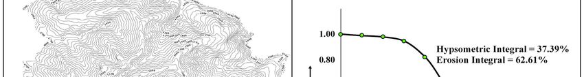
4.3.4 Hypsometric Analysis (Hs)
Langbein (1947) appear to have been the first to use such a line of study to collect hydrologic data. However, again
Strahler (1952) popularized it in his excellent paper. According to Strahler (1952) topography produced by stream
channel erosion and associated processes of weathering mass-movement, and sheet runoff is extremely complex,
both in the geometry of the forms themselves and in the inter-relations of the process which produce the forms. The
form of hypsometric curve and the value of the integral are important elements in topographic form. It show marked
variations in regions differing in stage of development and geologic structure, because in the stage of youth
hypsometric integral is large but it decreases as the landscape is denuded towards a stage of maturity and old age
(Strahler, 1952, pp. 118).
The authors used the percentage hypsometric method. It is a ratio of relative height and relative area with respect to
the total height and the total area of a drainage basin. It has been calculated with the help of following ratio:
a / A, where 'a' is the area enclosed by a pair of contours, and 'A ' is the total basin area which is represented on
the abscissa; and
h / H, where 'h' is the highest elevation between each pair of contours above the base, and 'H' is the total basin
height.
These data are shown in Table 7. The hypsometric curve was obtained in the graphical plots (Fig. 6).
Table 7: Hypsometric data of Tundah watershed
S. No. Altitude Range (m) Height (m) h Area (Kms2) a h / H, where H = 4050 a / A, where A = 284.83
1 5563 4050 7.57 1.00 0.03
2 5000-5563 3487 47.71 0.86 0.17
3 4500-5563 2987 110.33 0.74 0.39
4 4000-5563 2487 175.32 0.61 0.62
5 3500-5563 1987 234.28 0.49 0.82
6 3000-5563 1487 270.74 0.37 0.95
7 2500-5563 987 279.12 0.24 0.98
8 2000-5563 487 282.82 0.12 0.99
9 1513-5563 0 284.87 0.00 1.00
52Pareta and Pareta /International Journal of Remote Sensing and GIS, Volume 1, Issue 1, 2012, 41-56
Figure 6: Contour Map and Hypsometric curve of Tundah watershed, India
4.3.5 Hypsometric Integrals (Hi)
The hypsometric and erosion integrals calculated from the percentage hypsometric curve, give accurate knowledge
of the stage of the cycle of discussion. The following hypothetical standards have been recognized for determining
the stages (Table 8).
Table 8: Stages of Hypsometric Integrals
% of hypsometric integrals Stages
30 Old
30-60 Mature
60-80 Youth
80-100 Middle
100 Initial
The hypsometric integral (King, 1966, pp. 319-321) of Tundah watershed is 37.39% and the erosion integral of the
watershed is 62.61%, which indicates the mature stage of the Tundah watershed.
5. Conclusion
The study reveals that remotely sensed data i.e. CartoSAT-1 DEM and GIS based approach in evaluation of drainage
morphometric parameters and their influence on landforms, soils and eroded land characteristics at river basin level
is more appropriate than the conventional methods. GIS based approach facilitates analysis of different
morphometric parameters and to explore the relationship between the drainage morphometry and properties of
landforms, soils and eroded lands. Different landforms were identified in the watershed based on CartoSAT-1 DEM
data with 2.5m spatial resolution, and GIS software. GIS techniques characterized by very high accuracy of mapping
and measurement prove to be a competent tool in morphometric analysis. The morphometric analyses were carried
out through measurement of linear, areal and relief aspects of the watershed with more than 53 morphometric
parameters. The morphometric analysis of the drainage network of the watershed show dendritic and radial patterns
with moderate drainage texture. The variation in stream length ratio might be due to change in slope and
topography. The bifurcation ratio in the watershed indicates normal watershed category and the presence of
moderate drainage density suggesting that it has moderate permeable sub-soil, and coarse drainage texture. The
value of stream frequency indicate that the watershed show positive correlation with increasing stream population
with respect to increasing drainage density. The value of form factor and circulator ration suggests that Tundah
watershed is less elongated to oval. Hence, from the study it can be concluded that CartoSAT-1 (DEM) data,
coupled with GIS techniques, prove to be a competent tool in morphometric analysis.
53Pareta and Pareta /International Journal of Remote Sensing and GIS, Volume 1, Issue 1, 2012, 41-56
Acknowledgment
The authors are grateful to Kapil Chaudhery, Director Spatial Decisions New Delhi for providing the necessary
facilities to carry out this work. We are also thankful to Guru Ji Prof. J. L. Jain for the motivation of this work.
References
Agarwal, C.S. (1998). Study of drainage pattern through aerial data in Naugarh area of Varanasi district, U.P.,
Journal of Indian Society of Remote Sensing, 26, 169-175.
Babu, P.V.L.P. (1972). Photo-geomorphological analysis of the Dehra Dun valley, Bulletin, O.N.G.C. 9 (2), 51-55.
Black, P.E. (1972). Hydrograph responses to geomorphic model watershed characteristics and precipitation
variables, Journal of Hydrology, 17, 309-329.
Boison, O.J., and Patton, P.C. (1985). Sediment storage and terrace formation in Coyote Gulch basin, South-central
Utah, Geology, 1, 31-34.
Bukbank, D.W. (1983). The chronology of intermontane-basin development in the north-western Himalaya and the
evolution of the north-west Syntaxis, Earth and Planetary Science Letters, 64 (1), 77-92.
Chorely, R.J. (1957). Illustrating the laws of morphometry, Geological Magazine, 94, 140-150.
Christian, C.S. (1957). The concept of land units and land, 9th Pacific Science Congress. Department of Science,
Bangkok, Thailand, 20, 74-81.
Davis, W.M. (1902). River terraces in New England, In Jhonson, D.W. (ed.), Geographical Essays, London, Dover,
514-586.
De Terra, H. (1939). The quaternary terrace system of southern Asia and the age of man, Geographical Review, 29
(1), 101-118.
Dury, G.H. (1952). Methods of cartographical analysis in geomorphological research, Silver Jubilee Volume, Indian
Geographical Society, Madras, 136-139.
Faniran, A. (1968). The index of drainage intensity - A provisional new drainage factor, Australian Journal of
Science, 31, 328-330.
Gardiner, V. (1975). Drainage basin morphometry, British Geomorphological Group, Technical Bulletin, 14, 48.
Gilbert, G.K. (1877). Report on geology of the henry mountains, Washington, U.S. Geographical and Geological
Survey of the Rocky Mountain Region, 160.
Gravelius, H. (1914). Flusskunde, Goschen'sche Verlagshandlung, Berlin.
Gregory, K.J., and Walling, D.E. (1968). The variation of drainage density within a catchment, International
Association of Scientific Hydrology - Bulletin, 13, 61-68.
Hack, J.T. (1957). Studies of longitudinal profiles in Virginia and Maryland, U.S. Geological Survey Professional
Paper, 294 (B), 45-97.
Holland, T.H. (1907). A preliminary survey of certain glaciers in N.W. Himalayas, Records, Geological Survey of
India, 35 (3), 123-126.
Horton, R.E. (1932). Drainage basin characteristics, Transactions, American Geophysical Union, 13, 350-61.
Horton, R.E. (1945). Erosional development of streams and their drainage basins, Bulletin of the Geological Society
of America, 56, 275-370.
Howard, A.D. (1967). Drainage analysis in geologic interpretation: A summation, Bulletin of American Association
of Petroleum Geology, 21, 2246-2259.
Hynek, B.M., and Phillips, R.J. (2003). New data reveal mature, Integrated Drainage Systems on Mars Indicative of
Past Precipitation, Geology, 31, 757-760.
King, C.A.M. (1966). Techniques in geomorphology, Edward Arnold, (Publishers) Ltd. London, 319-321.
Krishnan, M.S., and Aiyengar, N.K.N. (1940). Did the Indo-brahm or Siwalik River exist?. Records, Geological
Survey of India, 75 (6), 24.
54Pareta and Pareta /International Journal of Remote Sensing and GIS, Volume 1, Issue 1, 2012, 41-56
Laity, J.E., and Malin, M.C. (1985). Sapping processes and the development of Theatre-Headed Valley networks on
the Colorado plateau, Bulletin, Geological Society of America, 96, 203-217.
Langbein, W.B. (1947). Topographic characteristics of drainage basins, U.S. Geological Survey Water Supply, 968
(C), 125-157.
Malin, M.C., and Edgett, K.S. (2000). Sedimentary rocks of early mars, Science, 290, 1927-1937.
Melton, M.A. (1957). An analysis of the relations among elements of climate, surface properties and
geomorphology, 389042 (11), Columbia University.
Melton, M.A. (1958). Geometric properties of mature drainage systems and their representation in E4 Phase Space,
Journal of Geology, 66, 35-54.
Miller, O.M. and Summerson, C.H. (1960). Slope zone maps, Geographical Review, 50, 194-202.
Mueller, J.E. (1968). An introduction to the hydrautic and topographic sinuosity indexes, Annals of the Association
of American Geographers, 58, 371-385.
Nag, S.K. (1998). Morphometric analysis using remote sensing techniques in the Chaka sub-basin, Purulia district,
West Bengal, Journal of Indian Society of Remote Sensing, 26 (1), 69-76.
Pareta, K. (2004). Geomorphological and hydro-geological study of Dhasan river basin, India, using remote sensing
techniques, Ph.D. Thesis, Dr. HSG University (Central University), Sagar (M. P.).
Rao, D.P. (2002). Remote sensing application in geomorphology, International Society for Tropical Ecology, 43(1),
49-59.
Schumm, S.A. (1956). Evolution of drainage systems & slopes in Badlands at Perth Anboy, New Jersey, Bulletin of
the Geological Society of America, 67, 597-646.
Sharp, R.P., and Malin, M.C. (1975). Channels on mars, Bulletin of the Geol. Society of America. 86, 593-609.
Shrivastava, P.K. and Bhattacharya, A.K. (2000). Delineation of groundwater potential zones in a hard rock terrain
of Bargarh district, Orissa - using IRS data. Journal Indian Society of Remote Sensing, Vol. 28(2&3), pp.
129-140.
Singh, N. (1990). Geomorphology of Himalayan rivers (a case study of Tawi basin), Jay Kay Book House, Jammu
Tawi.
Singh, S., and Dubey, A. (1994). Geo-environmental planning of watersheds in India, Allahabad, India: Chugh
Publications, 28 (A), 69.
Singh, S., and Singh, M.C. (1997). Morphometric analysis of Kanhar river basin, National Geographical Journal of
lndia, 43(1), 31-43.
Smart, J. S., and Surkan, A.J. (1967). The relation between mainstream length and area in drainage basins, Water
Resources Research, 3 (4), 963-974.
Smith, G.H. (1939). The morphometry of Ohio: The average slope of the land (abstract), Annals of the Association
of American Geographers, 29, 94.
Strahler, A.N. (1952a). Dynamic basis of geomorphology, Bulletin of the Geological Society of America, 63, 923-
938.
Strahler, A.N. (1952b). Hypsometric analysis of erosional topography, Bulletin of the Geological Society of
America, 63, 1117-42.
Strahler, A.N. (1956). Quantitative slope analysis, Bulletin of the Geological Society of America, 67, 571-596.
Strahler, A.N. (1957). Quantitative analysis of watershed geomorphology, Transactions-American Geophysical
Union, 38, 913-920.
Strahler, A.N. (1964). Quantitative geomorphology of drainage basin and channel network, Handbook of Applied
Hydrology, 39-76.
Strahler, A.N. (1968). Quantitative geomorphology, In: Fairbridge, R.W. (eds), The Encyclopedia of
geomorphology, Reinhold Book Crop, New York.
Strahler, A.N. (1980). Systems Theory in physical geography, Physical Geography 1, 1-27.
55Pareta and Pareta /International Journal of Remote Sensing and GIS, Volume 1, Issue 1, 2012, 41-56
Tomlinson, M.E. (1925). The river terraces of the lower Warwickshire Avon, Quarterly Journal of the Geographical
Society, 81, 137-169.
Wadia, D.N., and West W.D. (1964). Structure of the Himalayas, 22nd International Geological Congress, New
Delhi, 10, 1964.
Wentworth, C.K. (1930). A simplified method of determining the average slope of land surfaces, American Journal
of Science, 21, 184-194.
Wolman, M.G., and Miller, J.P. (1964). Magnitude and frequency of forces in geomorphic processes, Journal of
Geology, 68, 54-74.
Woodroffe, C.D. (1980). The lowland terraces, Geographical Journal, Vol. 146, 21-31.
56You can also read