Radio frequency emissions from dark matter candidate magnetized quark nuggets interacting with matter - Nature
←
→
Page content transcription
If your browser does not render page correctly, please read the page content below
www.nature.com/scientificreports
OPEN Radio frequency emissions
from dark‑matter‑candidate
magnetized quark nuggets
interacting with matter
J. Pace VanDevender1*, C. Jerald Buchenauer2, Chunpei Cai3, Aaron P. VanDevender4 &
Benjamin A. Ulmen5
Quark nuggets are theoretical objects composed of approximately equal numbers of up, down,
and strange quarks. They are also called strangelets, nuclearites, AQNs, slets, Macros, and MQNs.
Quark nuggets are a candidate for dark matter, which has been a mystery for decades despite
constituting ~ 85% of the universe’s mass. Most previous models of quark nuggets have assumed
no intrinsic magnetic field; however, Tatsumi found that quark nuggets may exist in magnetars as
a ferromagnetic liquid with a magnetic field BS = 1012±1 T. We apply that result to quark nuggets, a
dark-matter candidate consistent with the Standard Model, and report results of analytic calculations
and simulations that show they spin up and emit electromagnetic radiation at ~ 104 to ~ 109 Hz after
passage through planetary environments. The results depend strongly on the value of Bo, which is
a parameter to guide and interpret observations. A proposed sensor system with three satellites at
51,000 km altitude illustrates the feasibility of using radio-frequency emissions to detect 0.003 to
1,600 MQNs, depending on Bo, during a 5 year mission.
About 85%1 of the universe’s mass does not interact strongly with light; it is called dark matter, is distributed in
a halo throughout a g alaxy2. Identifying the nature of dark matter is currently one of the biggest challenges in
science. As reviewed most recently by Salucci3, extensive searches for a subatomic particle that would be consist-
ent with dark matter have yet to detect anything above background signals.
Most models assume dark matter interacts with normal matter only through gravity and the weak interac-
tion. However, detailed analysis of the accumulating data on galaxies of different types suggest dark matter and
normal luminous matter interact somewhat more strongly, on the time scale of the age of the Universe3. Magnet-
ized quark nuggets (MQNs)4 are an emerging candidate for dark matter that quantitatively meets the traditional
interaction requirements for dark matter and still interacts with normal matter on the time scale of the age of
the Universe through the magnetic force. In this paper we investigate a new method for detecting MQNs and
measuring their properties.
Quarks are the basic building blocks of protons, neutrons, and many other particles in the Standard Model of
Particle Physics5. Macroscopic quark n uggets6, which are also called s trangelets7, nuclearites8, AQNs9, slets10, and
11
Macros are theoretically predicted objects composed of up, down, and strange quarks in essentially equal num-
bers. A brief summary of quark-nugget research6–35 on charge-to-mass ratio, formation, stability, and detection
has been updated from Ref.16 and is provided for convenience as Supplementary Note: Quark-nugget research
summary.
Most previous models of quark nuggets have assumed negligible self-magnetic field. However, T atsumi15
explored the internal state of quark-nugget cores in magnetars and found that quark nuggets may exist as a fer-
romagnetic liquid with a surface magnetic field BS = 1012±1 T. Although his calculations used the MIT bag model
1
VanDevender Enterprises LLC, 7604 Lamplighter LN NE, Albuquerque, NM 87109, USA. 2Department of Electrical
and Computer Engineering, MSC01 1100, University of New Mexico, Albuquerque, NM 87131, USA. 3Department
of Mechanical Engineering and Engineering Mechanics, Michigan Technological University, MEEM 1013, 1400
Townsend Drive, Houghton, MI 49931, USA. 4Founders Fund, One Letterman Drive, Building D, 5th Floor,
Presidio of San Francisco, San Francisco, CA 94129, USA. 5Sandia National Laboratories, PO Box 5800, MS‑1159,
Albuquerque, NM 87115‑1159, USA. *email: pace@vandevender.com
Scientific Reports | (2020) 10:13756 | https://doi.org/10.1038/s41598-020-70718-3 1
Vol.:(0123456789)
www.nature.com/scientificreports/
with its well-known l imitations20, his conclusions can and should be tested. We have applied his ferromagnetic-
fluid model of quark nuggets in magnetars to magnetized quark nuggets (MQNs)4,16 dark matter and extend those
results to calculate how MQNs rotate and radiate radio frequency (RF) emissions during and after interaction
with normal matter. We also explore how the RF emissions can enable detection of MQNs.
As done in Ref.4, we will use Bo as a key parameter. The value of Bo is related to the mean value of the
surface magnetic field through.
ρQN ρDM_T=100 Mev
< BS >= Bo . (1)
1018 (kg/m3 ) 1.6 × 10⁸ (kg/m3 )
If MQN mass density ρQN = 1018 kg/m3 and the density of dark matter ρDM = 1.6 × 10⁸ kg/m3 at time t ≈ 65 μs
(when the temperature T ≈ 100 MeV in accord with standard ΛCDM cosmology), then Bo = . If better values
of ρQN, and ρDM are found, then the corresponding values of can be calculated with Eq. (1) from those better
values and from Bo determined by observations.
Previous papers on MQNs showed:
1. self-magnetic field aggregates MQNs with baryon number A = 1 into MQNs with a broad mass distribution4
that is characterized by the value of Bo and typically has A between ~ 103 and 1 037,
2. aggregation dominates decay by weak interaction so massive MQNs can form and remain magnetically
stabilized in the early universe even though they have not been observed in particle a ccelerators4,
3. the self-magnetic field forms a magnetopause that strongly enhances the interaction cross section of a MQN
with a surrounding p lasma16 that is primarily sustained by radiation and electron impact ionization in the
high temperature plasma formed by normal matter stagnating against the magnetopause,
4. Bo > 3 × 10¹² T is excluded4 by the lack of observed deeply penetrating impacts that deposit > Megaton-TNT
equivalent energy per km, so Tatsumi’s range of BS is reduced to 1 × 10¹¹ T ≤ Bo ≤ 3 × 10¹² T,
5. MQNs satisfy criteria for dark matter even with baryon’s interacting with MQNs through the self-magnetic
field4, and
6. the unexcluded range of Bo, the low (~ 7 × 10–22 kg m−3) density of local dark matter, net incident velocity
of ~ 250 km/s, and the high average mass of MQNs constrain the flux of MQNs of all masses to between 10–7
and 4 × 10–15 m−2 y−1 sr−1 and constrain the flux for MQN masses > 1 kg to between 3 × 10–14 and 2 × 10–17 m−2
y−1 sr−1, so very large area detectors or very long observation times are required4 to detect MQNs.
In this paper, we investigate the possibility of detecting MQNs interacting with the largest accessible target:
Earth, with its magnetosphere to 10 Earth radii. We show MQNs necessarily experience a net torque while pass-
ing through matter, can spin up to kHz to GHz frequencies, and emit sufficient narrow-band electromagnetic
radiation that could be detected in additional tests of the MQN hypothesis for dark matter.
Detection is also complicated by the magnetopause plasma (hot ionized gas) shielding some radio-frequency
(RF) emissions. Spacecraft re-entering the atmosphere cannot communicate with ground stations because the
surrounding plasma shields the emissions until the spacecraft slows down. The same blackout effect prevents
RF emissions from MQNs from being detected during the high-velocity interaction of MQMs with matter in
the troposphere or ionosphere.
However, MQNs that exit the atmosphere can be detected by their narrow-band, time-varying RF radiation,
with frequency equal to the rotation frequency. In addition, MQN detection rate should be strongly correlated
with the direction of dark-matter flux into the detector aperture. That preferred direction is determined by Earth’s
velocity about the galactic center and, consequently, through the dark-matter halo. These characteristics should
permit their detection and differentiation from background RF.
Results
In this section, we show (1) when MQNs interact with plasma, their rotational velocity increases as their transla-
tional velocity decreases, (2) MQNs passing through Earth’s atmosphere on a fly-by trajectory produce sufficient
RF emissions to be detected by satellites but not ground-based sensors, and (3) the frequency, RF power, and
event rate depend strongly on the value of the Bo parameter in Eq. (1).
Rotational spin‑up. Plasma is an ionized state of matter with sufficient electron number density ne at tem-
perature Te for the electrons and ions to behave as a quasi-neutral fluid. Quantitatively, that means there is at least
one electron–ion pair in a spherical volume of radius equal to a Debye shielding length λD,
εo kB Te
D = , (2)
ne e2
in which the permittivity of free space εo = 8.854 × 10⁻¹² F/m, the Boltzmann constant kB = 1.38 × 10⁻²³ J/K, and
electron charge e = 1.6 × 10⁻¹⁹ C. The Debye length is also the distance over which the thermal energy of the elec-
lasma36 versus an ensemble
trons permits charge separation to occur and defines electrical quasi-neutrality of a p
of electrons and ions which behave as particles. The distinction is important for MQNs. A plasma impacting the
magnetic field of a MQN acts as a conducting fluid and compresses the magnetic field to form a magnetopause16.
A co-moving electron–ion pair impacting the magnetic field will separate because the forces from their opposite
charges deflect them in opposite directions and will create a local electric field between them. The combined
force from their electric E and magnetic B fields causes them to move in the same E × B direction at the same
Scientific Reports | (2020) 10:13756 | https://doi.org/10.1038/s41598-020-70718-3 2
Vol:.(1234567890)
www.nature.com/scientificreports/
Figure 1. Generalization of the tan(χ) factor in Eq. (5), in which χ is the angle between the magnetic axis and
the normal to both the magnetic axis and the quark-nugget’s direction of travel in the rest frame of the quark
nugget. The solid red lines indicate the angles computed by Papagiannis; the solid blue lines indicate extensions
by symmetry. Dotted blue lines indicate functional extrapolation of Papagiannis and symmetry-extension
values.
velocity36 and through the magnetic field, instead of strongly compressing it. In contrast, conducting plasma
shorts out the electric field and prevents particle penetration.
A MQN moving through a plasma experiences a greatly-enhanced slowing down f orce16 through its mag-
netopause, which is the magnetic structure formed by particle pressure from a plasma stream balancing mag-
netic field pressure around a magnetic dipole. For example, the solar wind forms a magnetopause with Earth’s
magnetic field. Since the particles’ mean free path for collisions is much larger than the Larmor radius in the
magnetic field, the physics of Earth’s magnetopause is collisionless and applicable to the very small-scale lengths
of a quark-nugget’s magnetopause.
As derived in Ref.16, the cross section σm for momentum transfer by the magnetopause effect is
1
6
2Bo2 rQN 3
σm = 2
πrm =π (3)
µ0 ρx v 2
for magnetopause radius rm, MQN radius rQN, MQN speed v, and mass density of surrounding matter ρx. The
total force Fo exerted by the plasma on the quark nugget is approximately.
Fo ≈ σm ρx v 2 . (4)
Equations (3) and (4) let us calculate the decelerating force on the MQN and its translational velocity during
passage through matter16.
In this paper, we extend the dynamics to calculate the torque and rotational velocity of the MQN passing
through matter. P apagiannis37 showed that the solar wind, which has mass density ρx ≈ 10–20 kg/m3 and velocity
v ≈ 3.5 × 10⁵ m/s, exerts a torque T (N⋅m) on Earth (radius ro = 6.37 × 10⁶ m and magnetic field Bo = 3. × 10–5 T) as
a function of the angle χ between the magnetic axis and the normal to both the magnetic axis and the direction
of the solar wind. His semi-empirical result is expressed in MKS units as
T = C2 ρx0.5 vBo rQN
3
tan (χ ), (5)
in which C2 = 1,400 with units of Ns kg T . Papagiannis validated the expression for the angles χ within
−0.5 −1.5 −1
m
0.61 radians of 0 and within 0.61 radians of π (i.e. –0.61 ≤ χ ≤ + 0.61, –3.14 ≤ χ ≤ –2.53, and + 2.53 ≤ χ ≤ + 3.14, as
illustrated in Fig. 1). By symmetry of the magnetic field, the torque is 0 at χ = 0 and χ = ± π/2.
Since Papagiannis was only considering Earth, he limited his calculations to within 0.61 radians of the nor-
mal to the plasma velocity. Rigorously reproducing and extending his computational results to the larger angles
required for MQN rotation is beyond the scope of this paper. Therefore, we extend his results by observing the
amplitude of the torque is symmetric about χ = –3π/4, –π/4, π/4 and 3π/4, as shown in Fig. 1 by solid blue lines,
and approximate the rest of the torque function by extrapolation of the tan(χ) function in Eq. (5), as shown with
dotted blue lines in Fig. 1. The resulting functions Fχ and T, shown in Eq. (6), replace Eq. (5).
Scientific Reports | (2020) 10:13756 | https://doi.org/10.1038/s41598-020-70718-3 3
Vol.:(0123456789)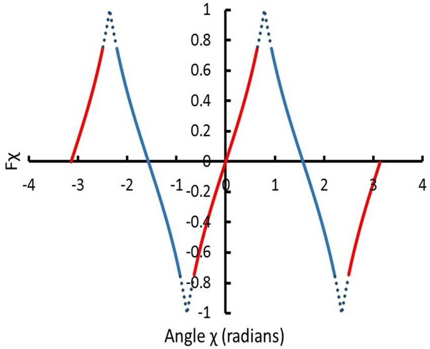
www.nature.com/scientificreports/
Figure 2. Calculated frequency versus time for 0.1 kg MQN with Bo = 2.25 × 10¹² T, initial velocity of 250 km/s,
and passing through air at density 1.0 kg/m3. Note the initial oscillation is about 0 until angular momentum
becomes sufficient to complete a full rotation.
tan χ
Fχ = MIN(ABS(tan χ), ABS(cot χ))
ABS(tan χ) (6)
T = C2 ρx0.5 vBo rQN
3
Fχ
The torque is negligible for Earth but is very large for a quark nugget. The rate of change of angular velocity
ω for MQN with mass mQN, moment of inertia Imom = 0.4 mQN rQN2 experiencing torque T is.
dω T
= . (7)
dt Imom
Equations (2)–(7) were solved for the angular velocity versus time. The interaction produces a velocity-
dependent and angle-dependent torque that causes MQNs to oscillate initially about an equilibrium. Since
the quark nugget slows down as it passes through ionized matter, the decreasing forward velocity decreases
the torque with time, so the time-averaged torque in one half-cycle is greater than the opposing time-averaged
torque in the next half-cycle. The amplitude of the oscillation necessarily grows, as shown in Fig. 2. Once the
angular momentum is sufficient to give continuous rotation, the net torque continually accelerates the angular
motion to produce a rapidly-rotating quark nugget. As shown in Fig. 2, MHz frequencies are quickly achieved
even with a 0.1 kg quark nugget moving through 1 kg/m3 density air at 250 km/s. For smaller or larger masses,
the resulting angular acceleration and velocity are respectively larger or smaller.
Several other approximations for the torque in the intervals shown with dotted lines in Fig. 1 gave the same
frequency within 5%, which is within the uncertainty of the magnetic field parameter Bo.
Equilibrium frequency and radiated power. Rotating magnetic dipoles emit electromagnetic radiation
in the far field with power per steradian38 given by
dP Zo ω
4 2
= mm sin2 χ (8)
d� 32π 2 c
in SI units, with Zo = 377 Ω, ω is angular frequency, and c is the speed of light in vacuum. The magnetic dipole
moment mm = 4π Bo rQN3/μo, and angle of rotation χ is the angle between the velocity of the incoming plasma and
the magnetic moment. The total power radiated38 is
Zo ω
4 2
P= mm . (9)
12π c
The spin-up process strongly depends on the details of the surrounding material mass and MQN velocity
along the path of the MQN, the MQN mass, and surface magnetic field Bo. In spite of these complexities, we
find that the spin-up time is very much less than the MQN transit time through the region of highest torque,
and the lower limit of final rotation frequency can be adequately estimated by assuming the energy gained per
cycle equals the energy radiated per cycle:
2π
ω
2πP
Tdt = , (10)
ω2
0
in which the torque T is given by Eq. (6) and the radiated power P is given by Eq. (9). Combining Eqs. (6)–(10)
gives
Scientific Reports | (2020) 10:13756 | https://doi.org/10.1038/s41598-020-70718-3 4
Vol:.(1234567890)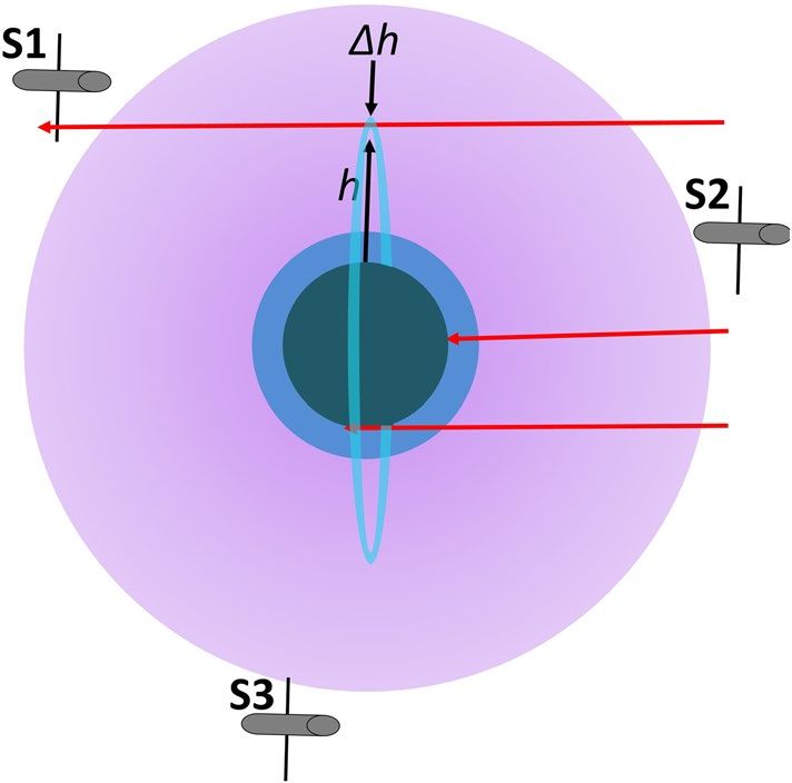
www.nature.com/scientificreports/
Figure 3. Near Earth environment with MQN trajectories (red lines). Three concentric circles represent MQN
interaction volume: highly ionized and low density magnetosphere and ionosphere (purple); weakly ionized
or neutral, low-density troposphere (blue), and neutral, high-density planet (gray). Satellites S1, S2 and S3 are
shown in orbits that let them monitor narrow-band RF emissions above background as described below. The
vertical ring (light blue) is a detection-area element for simulations of MQNs interacting with magnetosphere,
ionosphere and troposphere, as discussed below.
2π
ω 3
v(t)Fχ (χ(ωt)) 5.54x10⁻²² Bo rQN
dt = . (11)
ω2 ρx0.5
0
In the simulations discussed below, we solve Eqs. (3) and (4) for position and velocity v(t) calculated along
a trajectory through the atmosphere to the position of maximum density ρx, where we solve Eq. (11) for the
lower-limit to the maximum frequency ωmax.
Attenuation of RF power by magnetopause plasma. The surrounding magnetopause plasma has a
characteristic plasma frequency
12
4πne e2
1
ωpe = = 56.4ne2 , (12)
me
in which ne = the local electron number density, e = the electron charge, and me = the electron mass. The charac-
teristic e-fold length for attenuating the radiated power for frequency ω < ωpe is katten
−1
:
−1 c 1
katten =
2 . (13)
2ωpe
1 − ωωpe
In practice, the scale length 0.5c/ωpe is approximately 0.5% of the ion Larmor radius, which is approximately
the minimum thickness of the magnetopause boundary. Therefore, magnetopause plasma strongly absorbs RF
energy for frequencies less than the plasma frequency.
Since plasmas strongly absorb electromagnetic radiation with frequency less than the plasma frequency,
which varies with solar activity, practical detection of MQNs by their RF emissions is limited to ≥ 0.03 MHz in the
solar-wind plasma near Earth orbit, to ≥ 0.4 MHz in the magnetosphere, and to ≥ 40 MHz in the ionosphere. The
equilibrium frequency of the MQN spin-up process and the high density of the troposphere means, in practice,
all RF emissions in the troposphere are strongly shielded. Therefore, we will focus on detecting MQNs in the
magnetosphere after they have transited Earth’s atmosphere, as illustrated in Fig. 3.
The middle MQN trajectory in Fig. 3 represents a direct impact16. The bottom trajectory represents a MQN
that is gravitationally captured and does not exit into the magnetopause. The top trajectory represents a MQN
that spins up during transit and is detected by satellite S1. Satellite S2 would not detect these MQNs since they
have not passed through sufficient matter to spin up. Therefore, appropriate differences in event rates as a func-
tion of satellite position would support detection of dark matter.
Trajectories of quark nuggets are from a preferred direction in Fig. 3 because the velocity of the solar system
about the galactic center and through the halo of dark matter nearly dominates the random velocity of quark
nuggets, as discussed in a subsequent section.
Scientific Reports | (2020) 10:13756 | https://doi.org/10.1038/s41598-020-70718-3 5
Vol.:(0123456789)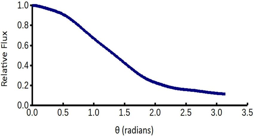
www.nature.com/scientificreports/
Radiofrequency background from MQNs distributed throughout the galaxy. Dark-matter is
distributed throughout the galaxy2,3. Therefore, MQN dark matter in interstellar space might interact with the
local plasma density and emit RF radiation that fills the universe over billions of years. The resulting RF might
be detectable as a galactic background near Earth. Olbers’ Paradox on why the night sky is dark39 addresses the
same phenomenon for photons from stars. Evaluating the potential for detecting and interpreting this radia-
tion is complex. A detailed analysis is beyond the scope of this paper, which focuses on detection of near-Earth
MQNs. However, the following preliminary analysis shows that the MQN hypothesis cannot be tested by obser-
vations of galactic RF background near Earth.
The plasma density and temperature in interstellar space vary greatly:
1. a minimum of ~ 10–4 to ~ 10–2 particles/cm3 in Hot Ionized Media (HIM) at Te ~ 106 to 107 K composing 20%
to 70% of interstellar space,
2. to ~ 0.2 to 0.5 particles/cm3 in Warm Ionized Media (WIM) at Te ~ 8,000 K composing 20–50% of space,
3. to higher mass densities represented by ~ 102 to 1 06 particles/cm3 in molecular clouds at Te ~ 10 to 20 K
composing < 1% of space40.
As discussed above, matter has to act like a fluid plasma (instead of an ensemble of isolated charged particles)
to form a magnetopause. Quantitatively, the scale length λD for charge separation in Eq. (2) has to be less than
the magnetopause radius rm defined in Eq. (3), so
1
1
rm Bo mQN ne 3 1 2
= 4000. > 1. (14)
D ρQN v Te
For example, using the mid-range value of Bo = 2.0 × 10¹² T and ρQN = 1 × 10¹⁸ kg/m3, the MQN mass has to be
greater than 1 07 kg for a magnetopause to form in HIM. The equilibrium rotation frequency for such massive
MQNs is much less than 30 MHz and the corresponding RF is absorbed by the solar-wind plasma near Earth.
The corresponding threshold MQN mass for forming a magnetopause in WIM is 10 kg. However, the higher
density plasma in the WIM slows those MQNs, so their RF is still less than 30 kHz, so it is also absorbed in the
solar-wind plasma near Earth.
In general, the larger mass density of the rest of interstellar media produce even lower frequency RF, which is
absorbed even further from Earth. We analyzed these effects for the full range of interstellar plasma conditions40
and MQN mass distributions4 as a function of the Bo parameter. We found wherever MQN dark matter can
produce RF emissions, the emissions are either absorbed in the surrounding plasma or in the solar-wind plasma
near Earth. The RF is not detectable near Earth and cannot be used to test the MQN hypothesis. Therefore, we
focus on detecting MQNs passing very near Earth and radiating well above the 30-kHz cutoff frequency of the
solar-wind plasma.
Discriminating MQN events from background. Theoretical profiles of dark matter halos are guided by
astrophysical observations, which are consistent with a mass density of dark matter near Earth of about 7 × 10–
22
kg/m3 ± 70%3,14. This extremely low mass density and the very broad mass d istributions4 mean that the flux of
MQNs is very low. Detecting them over the full range of not-excluded values of Bo requires interaction volumes
of at least planetary size and requires a means of reliably subtracting background. The orientation of the sensed
MQN flux with respect to the direction of inflowing dark matter provides one such opportunity.
Models differ in their degree of self-interaction. Computer s imulations41 covering a substantial portion of
these models indicate dark matter occupies a halo within and around the galaxy’s ordinary matter and has a
Maxwellian-like, isotropic velocity distribution. Although simulations predict the velocity distribution of dark
matter varies somewhat with the self-interaction model, the most probable, isotropic speed is ~ 220 km/s with a
full-width-at-half-maximum of ~ 275 km/s.
The solar system moves through this high-speed dark-matter halo in its ~ 250 km/s motion about the galactic
center. The direction of this motion is towards the star Vega, which has celestial coordinates: right ascension
18 h 36 m 56.33635 s, declination + 38° 47′ 01.2802″. In addition, Earth moves around the Sun at ~ 30 km/s. The
vector sum of these two velocities gives the net velocity of Earth through dark matter, and the negative of this
vector sum is the velocity of dark matter relative to Earth, shown in Fig. 4 for the position of Earth on the first
day of each month.
A sensor on Earth should detect the most events per hour when it is sensitive to the flux of dark matter from
the direction of Vega and much less when Earth shields the detector from the flux. A satellite in orbit about Earth
would encounter a higher flux of MQNs when it is not shielded by Earth and when it is within range of MQNs
that have transited through enough matter to spin up, as illustrated by S1 in Fig. 3.
The dark-matter velocity distribution has a streaming component Us relative to the sensor and an isotropic
component Uiso relative to the galactic center. The isotropic component smooths the transition between the
directly exposed and Earth-shielded conditions.
Uiso can be adequately approximated for our purposes as the
highest probability thermal speed Uiso = 2kT M of a 3D Maxwellian velocity distribution of dark matter with
mass M and with temperature T, where k is the Boltzman constant. S imulations41 indicate that Us ≈ Uiso. Therefore,
we calculated the detection rate as a function of the sensor’s orientation on Earth with respect to Vega and
S = Us/Uiso using the method developed by Cai et al.42. The results are shown in Fig. 5.
Scientific Reports | (2020) 10:13756 | https://doi.org/10.1038/s41598-020-70718-3 6
Vol:.(1234567890)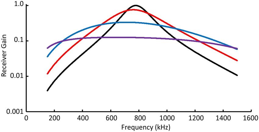
www.nature.com/scientificreports/
Figure 4. For the first day of each month, Earth’s position and velocity about the Sun are shown. The solar
system’s velocity towards Vega is shown by the black vector from the Sun. The net velocity vector of dark matter
into Earth is shown in blue for each month. The effects of the 23.5° angle between Earth’s equatorial plane and
the ecliptic and the 38.8° angle between Earth’s equatorial plane and Vega’s position are not shown.
Figure 5. Calculated and normalized variation of dark matter flux streaming from the direction of the star Vega
as a function of polar angle θ from Vega’s zenith.
If this variation with respect to Vega’s position is observed, i.e. the event rate for satellite S2 in Fig. 3 is appro-
priately and systematically less than the event rate for S1, the result would be convincing evidence of having
detected MQN dark matter.
Including MQNs from all directions. The flux in Fig. 5 is normalized to Fθ=0, the total number of events
m−2 y−1 sr−1 for a detection surface facing directly into the streaming velocity Us, and was approximated from the
mass distributions in Ref.4, assuming the mean incoming velocity Us = 2.5 × 10⁵ m/s and assuming the effect of
Uiso ≠ 0 on the flux is negligible to first order for θ = 0. Assuming cylindrical symmetry in azimuthal direction φ
and integrating the curve in Fig. 5 over solid angle with dΩ = sinθ dθ dφ gives the correction factor for estimating
the event rate in m−2 y−1 for MQNs incident from all directions
π
Fall_� = 2π Fθ =0 dθ = 5.56. (15)
0
The results of the simulation for θ = 0 in subsequent sections are multiplied by 5.56 to estimate the event rate
for MQNs from all directions.
Scientific Reports | (2020) 10:13756 | https://doi.org/10.1038/s41598-020-70718-3 7
Vol.:(0123456789)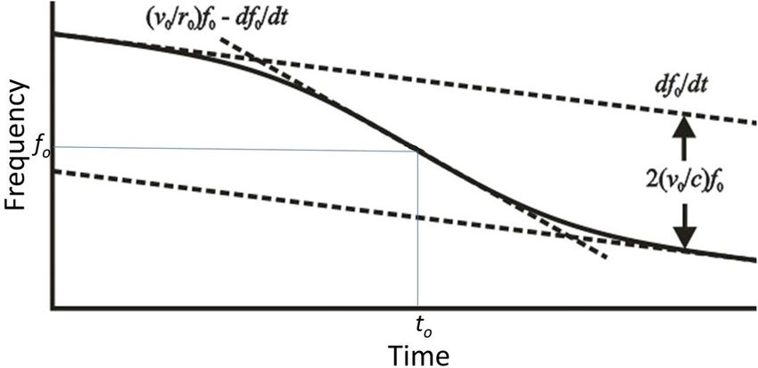
www.nature.com/scientificreports/
Figure 6. Data points for RF power as a function of maximum equilibrium frequency for MQNs transiting
through Earth’s atmosphere for four representative values of Bo are enclosed within the four perimeters: solid
blue for Bo = 3.0 × 10¹² T, dashed blue for Bo = 2.5 × 10¹² T, dashed red for Bo = 2.0 × 10¹² T, and dotted red for
Bo = 1.5 × 10¹² T.
Simulating MQNs flying by Earth. Consider the simple case of a quark-nugget with a trajectory parallel
to a tangent to Earth, as illustrated by the three trajectories in Fig. 3. Satellites sense MQNs after they have trans-
ited the highest density matter along their trajectories and experienced the corresponding torque, as described
in Eq. (6), to produce the maximum frequency and radiated power. After they pass into the magnetosphere, they
can be detected since their emissions above ~ 0.4 MHz are no longer shielded by the higher-density plasma of
the ionosphere.
In our simulations, Earth’s atmosphere is divided into increments ∆h of altitude h. MQN trajectories are
characterized by their minimum altitude for 0 < h ≤ 9 re, for re = 6.378 × 10⁶ m, which is one Earth radius. For
each increment ∆h, test MQNs with masses consistent with the mass distributions of Ref.4 are injected from
the right in Fig. 3 with initial velocity in the x direction vx = -Us = -2.5 × 10⁵ m/s. Their positions and velocities
are calculated under the combined effects of gravity and magnetopause interaction. For each test particle, the
maximum torque encountered in its trajectory, i.e. the torque in Eq. (6) at the maximum value of the product of
total velocity and the square root of the local mass density, is used to calculate the equilibrium frequency from
Eq. (11) and the corresponding RF power from Eq. (9).
Characteristic times τup = ωmax Imom/Tmax for spin up and τdown = 0.5 Imom ωmax2/Pmax for spin down by radiation
loss are calculated. Since we find τup is much less than transit time through the atmosphere, ωmax is the lower
limit to the maximum frequency, from Eq. (11). The value of τdown helps determine the detectability of each rep-
resentative MQN. Characteristic e-fold times for spin up and spin down are included in Supplementary Results:
Representative Data Tables for Sensor Design. Values of τdown vary from a minimum of 2.4 × 10³ s to a maximum
of 1.9 × 10⁶ s and provide adequate time for detection.
The cylindrically symmetric cross sectional area Ah associated with the altitude increment ∆h and altitude h
above Earth radius re is illustrated in Fig. 3 and is given by
Ah = 2π(re + h)(�h). (16)
MQNs with final velocity exceeding low-Earth orbital velocity ≥ 7,400 m/s escape the RF-absorbing iono-
sphere and will be recorded by a satellite-based sensor.
Atmospheric density as a function of altitude h = r – re for MQNs at radius r and Earth radius re were derived
from the literature and fit with the following equations:
For radius r below the magnetosphere43, i.e. 0 > r – re > 2.873 × 10⁵ m:
ρatm = 1.0 exp(−(r − re )/7.25x103 ) (17)
and for radius r in the magnetosphere44, i.e. 2.873 × 10⁵ m > r – re > 10 re:
r
ρatm = 1.6 × 10⁻¹⁷ 10−0.285714 re (18)
Mass density in Earth’s magnetosphere depends strongly on solar activity and varies greatly. The data in Ref.44
were averaged to produce Eq. (18), which should be adequate to estimate the annual event rate.
Our simulations show MQNs radiating between 10–28 W and 10+13 W and at frequencies between 0.35 MHz
and ~ 2 GHz. Very high frequencies are associated with negligible RF power, and very high powers are associated
with frequencies that are shielded by the magnetopause plasma. Results for RF power as a function of frequency
are shown in Fig. 6 for events radiating at more than 1 μW and at frequencies more than 100 kHz. Results are
shown for four representative and non-excluded values of Bo.
As shown in Fig. 6, highest power emissions occur at the lowest frequencies and highest values of Bo. These
originate from the most massive MQNs penetrating the troposphere, but there are very few of them. The map
associated with Bo = 1.5 × 10¹² T is common to the maps of all Bo values. The differences represent aggregation
run-away as discussed in Ref.4.
Figure 6 represents events by frequency and RF power but does not indicate the expected number of events
per year. For each test MQN, the effective target area, given by Eq. (16), was multiplied by the corresponding
Scientific Reports | (2020) 10:13756 | https://doi.org/10.1038/s41598-020-70718-3 8
Vol:.(1234567890)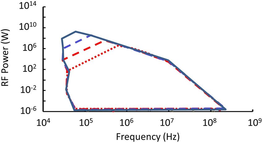
www.nature.com/scientificreports/
Figure 7. Number of events per year expected, from all directions, above the indicated detection threshold
of RF power for MQNs transiting through Earth’s atmosphere for four representative values of Bo: solid
blue for Bo = 3.0 × 10¹² T, dashed blue for Bo = 2.5 × 10¹² T, dashed red for Bo = 2.0 × 10¹² T, and dotted red for
Bo = 1.5 × 10¹² T.
number flux from Ref.4 and by the 5.56 factor from Eq. (15), and summed over all simulated events with RF
power greater than a sensor’s detection threshold to estimate the number of events that might be observable per
year as a function of detection threshold. The results are shown in Fig. 7.
At 1 nW threshold, the number of events per year that might be detectable in space out to 10 re
is ~ 30,000, ~ 8, ~ 0.8, and ~ 0.01 for Bo = 1.5 × 10¹² T, 2.0 × 10¹² T, 2.5 × 10¹² T, and 3.0 × 10¹² T, respectively. For 1 μW
detection threshold, the number events per year drops to ~ 10,000, ~ 7, ~ 0.07, and ~ 0.003 for Bo = 1.5 × 10¹² T,
2.0 × 10¹² T, 2.5 × 10¹² T, and 3.0 × 10¹² T, respectively.
The number of events per year decreases so strongly with increasing Bo because larger values of Bo cause faster
aggregation of MQNs in the early universe and, consequently, larger mass M QNs4. Since the mass per unit volume
of dark matter is constrained by observations to be ~ 7 × 10–22 kg/m3, the number density of MQNs decreases for
increasing mass and increasing Bo. So the flux of MQNs and detection rate decrease for increasing Bo.
Detailed results for MQNs with RF power greater than 1 nW and with sufficient flux to be in the most prob-
able 80% of events are provided in Supplementary Results: Representative Data Tables for Sensor Design. The
information should be useful for designing sensors for detecting MQNs.
Baseline sensor system. A realistic sensor system is, of course, essential for testing the MQN dark-matter
hypothesis. A convenient coincidence of frequency range and emerging technology enable a practical sensor. We
outline one such baseline system and compute the corresponding event rate in this section.
As shown in Fig. 3, the system has three satellites equally spaced in a circular orbit with inclination 38.783°
(to match MQN flux) at 51,000 km altitude where (1) the background plasma density is sufficiently low to permit
good RF propagation in the intended detection band of 1 05 to 1 06 Hz, (2) radiation damage from electrons in the
outer Van Allen belt is minimized, and (3) coverage by three satellites is acceptable. The Interplanetary Monitor-
ing Platform IMP-6 (Explorer 43) spacecraft45,46 is the reference architecture for the sensor system’s spacecraft.
IMP-6 was a 16-sided drum, 1.8-m long by 1.35-m diameter, having four 46-m long monopole antennas operating
in pairs as 91 m long dipoles, and spinning at 5.4 revolutions per minute to scan space. Our baseline design is
the same architecture but with 350 m long dipoles.
The sensor is based on the standard radar equation, formulated as transmit-receive equation:
c2 Ps
Pr = Gr Gs (19)
4πf 2 4πR2
where Pr is the received power, f is the frequency in Hz, c is the speed of light, Gr is the antenna gain, Ps is the
source power, R is the distance, and Gs is the source gain, which will be taken to be unity to represent the time
averaged value. Lossless dipoles up to a half-wavelength long have gains Gr < 1.6 and directivities Dr from 1.5 to
1.6. The weak signals require amplification in the receiver. The noise power PN and the signal to noise ratio S/N
for an amplified receiver are
Gr
PN = kB Tnoise f + kB Ta f (20)
Dr
Scientific Reports | (2020) 10:13756 | https://doi.org/10.1038/s41598-020-70718-3 9
Vol.:(0123456789)www.nature.com/scientificreports/
F (MHz) 0.2 0.3 0.5 0.8 1.0 2.0 3.0
Tnoise (MK) 3.1 6.2 21 24 19.5 8.2 4.0
Cane47 Tnoise (MK) < 7.3 11 15–38 18–27 16–23 6–11 2.6–5.0
Table 1. Radiation temperature in millions of Kelvin degrees for various frequencies.
2
S c P
=
s
(21)
N 4πRf kB Tnoise �f Dr + kB Ta �f Gr
where Boltzmann’s constant kB = 1.38 × 10⁻²³ J/K, Tnoise is the absolute radiation noise temperature, Ta is the
preamplifier noise temperature, and △ f is the receiver resolution bandwidth.
Solving Eq. (21) for the range R gives
−1
c Gr Gs Ps c Ps S
R=
=
. (22)
4πf S N 4πf kB Tnoise �f Dr + kB Ta �f Gr N
Since many measurements will be made on each MQN as it transits through detection range, we can oper-
ate at signal/noise ratio S/N = 1 and use signal averaging and pattern recognition to reliably detect the signal.
The background noise temperature Tnoise is a major factor in determining sensor performance. IMP-6 meas-
ured the galactic background noise in the magnetosphere between 354 km and 206,000 km altitude and between
130 and 2,600 kHz. To determine noise temperatures from the noise power measurements of Brown45, we equate
his values for spectral brightness B to the brightness in the Rayleigh-Jeans law for blackbody radiation and solve
for the noise temperature Tnoise
2kB f 2 Tnoise c2
3.26 × 10²¹
B or Tnoise Mo K = 2 (23)
B= , so Tnoise = B
c 2 2kB f 2 f (MHz)2
The results are shown in Table 1. The frequency range of interest encompasses a temperature maximum of 24
million degrees (MK) near 0.8 MHz. Ground based measurements at the poles during solar minima by Cane47
are also shown in Table 1 for comparison and are consistent with our analysis of Brown’s45 data.
Researchers accustomed to working at much higher frequencies, e.g. in satellite communications or radio
astronomy, may find these values of Tnoise to be unreasonably high. However, Tnoise is decreasing from 0.8 MHz
to 3.0 MHz in Table 1; it continues to decrease with increasing frequency to agree with Tnoise observed in those
disciplines.
Fitting the data with the minimum of two polynomials reproduces the table for 0.2 MHz ≤ f ≤ 3.0 MHz
within ± 1% and provides a useful function for estimating sensor performance:
Tnoise = min(659.03f 4 − 1627.9f 3 + 1313.5f 2 − 359.49f + 34.4, 40.0f −2 )MK (24)
For these low frequencies f (MHz), the noise temperature is millions of degrees Kelvin. From the denominator
under the square-root term in Eq. (22), we see that variation of range with antenna gain is small if
Ta
Gr ≥ Dr . (25)
Tnoise
Since noise temperature T a can be less than 100 K (which does not require a cryogenic amplifier) for the
frequencies of interest, 25 MK > Tnoise > 3 MK in Table 1, and Dr ~ 1.5, Eq. (23) gives 6 × 10⁻⁶ < Gr < 5 × 10⁻⁵ before
the range becomes very sensitive to antenna gain. For source powers of 1·w, antenna gains of 0.001 to 1, radia-
tion noise temperatures of 10 million K for the present case, amplifier noise temperatures of 100 K, receiver
bandwidths of 1 Hz, and signal to noise ratios of unity, one gets ranges of 14,954 km and 15,740 km at 0.5 MHz.
Therefore, range is very insensitive to antenna gain, and antenna gains that are well below unity are acceptable
when the radiation temperature is very high.
The antenna gain Gr depends on the dimensions and the termination impedance of the dipole antenna.
Tang, Tieng, and Guna’s t heory48 was used to design the antenna subsystem. The antenna gain Gr as a function
of frequency is shown in Fig. 8 for four terminating impedances.
For a wide range of terminating impedances, Gr easily satisfies Eq. (25) and the simple dipole is suitable for
the baseline system. The optimal dipole design will likely incorporate resistive and/or possibly reactive loading at
discrete positions along its length to achieve the best bandwidth and gain response if the additional complexity
does not preclude deployment in space.
The other variables in Eq. (22) are source gain Gs and signal-to-noise ratio (S/N). Both are set to 1.0. For
multiple measurements like the satellites will be recording, detections with S/N = 1 are routine, and detections
have been demonstrated for S/N as low as 0.1.
We found two options that apparently meet key requirements for the receiver: Δf = 1 Hz and a million simul-
taneously recorded frequencies. Assuming that such compact and low-power, ground-based electronic hardware
can be made into space-qualified hardware, they provide proof-of-principle of receiver feasibility. The Tektronix
RSA 306B Real Time Spectrum Analyzer system with Tektronix proprietary software on a separate computer
Scientific Reports | (2020) 10:13756 | https://doi.org/10.1038/s41598-020-70718-3 10
Vol:.(1234567890)www.nature.com/scientificreports/
Figure 8. Antenna gain is shown as a function of frequency for a load impedance of 65 Ω (black line), 195 Ω
(red line), 650 Ω (blue line), and 1950 Ω (purple line). The matched impedance is 65 Ω.
monitors 106 frequencies every 2 s with the required bandwidth Δf = 1 Hz and outputs the results to a laptop
computer. In addition, the N210 USRP unit from National Instruments, which we have been using for autono-
mous data collection with our custom software for 254 frequencies every 25 μs, can meet the requirements by
replacing the Field Programmable Gate Arrays (FPGAs) currently used for processing fast Fourier transforms
with General Purpose Computing on Graphics Processing Units (GPGPUs).
In both cases, processing the data on 1 06 simultaneous frequencies to find the unique signature of an MQN
and extract the desired information will be a significant challenge. A combination of on-board processing with
GPGPUs to select data for download and ground-based post-processing should be sufficient but has yet to be
demonstrated.
Estimated MQN detection rates. Although the non-excluded range for Bo at the time of this publica-
tion is 1 × 10¹¹ T ≤ Bo ≤ 3 × 10¹² T, recent results being prepared for publication reduce the non-excluded range to
1.5 × 10¹² T ≤ Bo ≤ 3 × 10¹² T. If Bo < 1.5 × 10¹² T is included, the predicted MQN detection rate will be even larger
and will shift to higher frequencies.
The number of events expected with the three-satellite sensor system described in this section was calculated
for four values of Bo in the more limited range. The calculation includes (1) computed number, frequency, and
RF power of fly-through MQNs, (2) the measured RF background temperature as a function of frequency, (3)
the sensor range as a function of MQN frequency and RF power from Eq. (22), and (4) the fraction of the area
monitored by the three satellites at the 51,000-km altitude of their orbit as a function of MQN frequency and
RF power. The number of MQNs that should be detected in five years of observations for 0.1–1.1 MHz RF as a
function of Bo:
• 1,620+ /− 40 if Bo = 1.5 × 10¹² T,
• 8.1+ /− 2.8 if Bo = 2.0 × 10¹² T,
• 0.05+ /− 0.2 if Bo = 2.5 × 10¹² T, and
• 0.003+/− 0.6 if Bo = 3.0 × 10¹² T.
Since quark nuggets are also baryons, their magnetic field may be similar to that of protons, which have the
equivalent magnetic field Bo between 0.9 × 10¹² T and 2.2 × 10¹² T.
The case for Bo = 1.5 × 10¹² T is quite different because the corresponding MQN mass is much smaller, so
the flux is much larger and the frequencies are much higher. Approximately 7% of events are between 0.1 and
1.0 MHz, 26% are between 1 and 3 MHz, 54% are between 3 and 10 MHz, and 13% are from 10 to 200 MHz. The
system should be optimized for 0.1 to 1.0 MHz. If the RF background permits some additional measurements
between 1 and 200 MHz would explore the special case of Bo ~ × 1012 T, unless additional observations in the
near future exclude that case.
Obtainable measurements and information. MQNs transiting through the magnetosphere, as shown
in Fig. 3, provides a frequency source f0(t) moving at constant non-relativistic velocity v in a straight line. A sta-
tionary observer at distance r(t) records the observed frequency versus time. The closest approach occurs at time
t0 and at distance r0. The observed frequency f (t) will be
v v t ′
0 0 � �
f0 t ′ , with f (t) ∼
�
f (t) = 1 + � = f0 + f (t − t0 ) and t ′ = t − t0 − r0 c. (26)
c 2
r0 + v0 t2 ′2
Total Doppler shifts are expected to be about that 1.5% of f0. The source frequency is expected to decrease
with time. During the brief periods of detectability, the source frequency should change linearly with time by
amounts comparable to or less than the Doppler shifts.
Scientific Reports | (2020) 10:13756 | https://doi.org/10.1038/s41598-020-70718-3 11
Vol.:(0123456789)www.nature.com/scientificreports/
Figure 9. Observed Doppler shifted frequency versus time for source radiating at f0 = unshifted frequency,
moving with v0 = relative velocity, passing at r0 = distance of closest approach at time t0. Dotted lines show
asymptotic rate of change of frequency df0/dt well before and after closest approach.
Figure 9 shows what can be extracted from measurements of frequency versus time from the moving source.
The velocity v0 is determined from the asymptotic limit lines. The slope of these lines determines the rate of
change of frequency of the source. The location of the inflection point determines f0 and t0, and the slope of the
central asymptote determines (v0/r0)f0 – df0/dt from which r0 is determined with the other measured variables.
Because signal strengths are not likely to be measurable in the far asymptotic regions, it is important that
good data be observed in the regions of maximum d2f/dt2, which occur at distances less than 2r0. Optimal fits of
data to Eq. (26) will provide estimates of the variables of interest.
Thus, from the measurement it is possible to estimate t0, f0, df0/dt, r0, v0, and dv0/dt and analyze the data to
get two measurements of MQN mass, one from f0 and df0/dt and one from v0 and dv0/dt. With enough data the
MQN mass distribution can be constructed and compared with the predictions in Ref.4 and be used to refine
Tatsumi’s value of the surface magnetic field in magnetar cores.
Discussion
We have shown that MQNs transiting through ionized matter experience a torque on their magnetopause and
spin up to high frequencies, ranging from kHz to GHz, depending on MQN mass and velocity, mass density
of the surrounding matter, and the Bo parameter. Rotating MQNs radiate. If the radiation is above the plasma
frequency of the surrounding matter, the RF radiation will propagate and can, in principle, be used to detect
MQN dark matter at a substantial distance.
We did examine the possibility of using ground-based sensors to detect MQNs transiting the magnetosphere
and radiating at > 40 MHz, the cut-off frequency of the ionosphere. The event rate is at most 0.3, 0.02, 0.0004,
and 0.00007 per year even if 2π steradians solid angle can be observed. A space-based system is more promising.
Our results have identified requirements for MQN detection systems and a baseline system of three satellites
that should test the MQN hypothesis for dark matter by detecting between 1,600 and 0.003 MQNs for Bo between
1.5 × 10¹² T and 3.0 × 10¹² T, respectively. Recording their Doppler shifted frequencies during their passage by a
sensor provides two different measurements of the MQN mass, so a mass distribution can be obtained in time.
The pattern of trajectories with respect to the direction of Vega, frequency, and rate of change of frequency
would provide strong evidence of MQNs and eventually characterize the actual mass distribution of MQNs to
compare with the predictions of Ref.4.
Very low mass MQNs will have frequencies of up to 2 GHz, but their negligible RF power precludes their
being detected. Very high mass MQNs will emit RF power of up to 1 013 W, but their negligible flux makes their
detection unlikely in a year of observation. As shown in Supplementary Results: Representative Data Tables for
Sensor Design, frequencies between 100 and 800 kHz are the most likely frequencies to be observed from MQNs.
Discerning quark-nugget signals from all human-caused and naturally occurring, non-MQN RF is facilitated
by their characteristics: (1) narrow-band RF, unlike RF from lightning and other discharges, (2) continuous emis-
sions, unlike pulsing radars, (3) relatively unmodulated in frequency and amplitude, unlike communication RF,
(4) moving at ~ 200 km/s, unlike all human sources, and (5) initially increasing in frequency to a maximum and
then slowly decreasing, unlike magnetosonic waves.
Finally, we note that solar and planetary atmospheres can be even larger-area, but less accessible, targets for
RF-emitting MQNs.
Data availability
All final analyzed data generated during this study are included in this published article with its Supplements.
Received: 10 May 2020; Accepted: 3 August 2020
Scientific Reports | (2020) 10:13756 | https://doi.org/10.1038/s41598-020-70718-3 12
Vol:.(1234567890)www.nature.com/scientificreports/
References
1. Aghanim, N. et al. (Planck Collaboration), Planck 2018 results. VI. Cosmological parameters (2018). arXiv: 1807.06209. pdf (2018).
Accessed 10 May 2020.
2. Navarro, J. F., Frenk, C. S. & White, S. D. M. The structure of cold dark matter halos. Astrophys. J. 462, 563–575 (1996).
3. Salucci, P. The distribution of dark matter in galaxies. Astron. Astrophys. Rev. 27, 2 (2019).
4. VanDevender, J. P., Shoemaker, I., Sloan T., VanDevender, A. P. & Ulmen, B.A. Mass distribution of magnetized quark-nugget dark
matter and comparison with requirements and direct measurements. arXiv:2004.12272 (2020). Accessed 10 May 2020.
5. Oerter, R. The Theory of Almost Everything: The Standard Model, the Unsung Triumph of Modern Physics (Penguin Group, London,
2006).
6. Witten, E. Cosmic separation of phases. Phys. Rev. D 30, 272–285 (1984).
7. Farhi, E. & Jaffe, R. L. Strange matter. Phys. Rev. D 30, 2379–2391 (1984).
8. De Rủjula, A. & Glashow, S. L. Nuclearites—a novel form of cosmic radiation. Nature 312, 734–737 (1984).
9. Zhitnitsky, A. “Nonbaryonic” dark matter as baryonic color superconductor. JCAP 0310, 010 (2003).
10. Xia, C. J., Peng, G. X., Zhao, E. G. & Zhou, S. G. From strangelets to strange stars: a unified description. Sci. Bull. 61, 172 (2016).
11. Jacobs, D. M., Starkman, G. D. & Lynn, B. W. Macro dark matter. MNRAS 450, 3418–3430 (2015).
12. Wandelt, B. D. et al. Self-interacting dark matter. In Ch. 5 Sources and Detection of Dark Matter and Dark Energy in the Universe,
from 4th International Symposium, Marina del Rey, CA, USA, February 23–25, 2000, (ed. Cline, D. B.) 263–274. (Springer, 2001).
arXiv :astro-ph/0006344, (2000). Accessed 10 May 2020.
13. McCammon, D. et al. A high spectral resolution observation of the soft x-ray diffuse background with thermal detectors. Astrophys.
J. 576, 188 (2002).
14. Tulin, S. Self-Interacting dark matter. AIP Conf. Proc. 1604, 121 (2014).
15. Tatsumi, T. Ferromagnetism of quark liquid. Phys. Lett. B 489, 280–286 (2000).
16. VanDevender, J. P. et al. Detection of magnetized quark nuggets, a candidate for dark matter. Sci. Rep. 7, 8758 (2017).
17. Lugones, G. & Horvath, J. E. Primordial nuggets survival and QCD pairing. Phys. Rev. D 69, 063509 (2004).
18. Steiner, W. S., Reddy, S. & Prakash, M. Color-neutral superconducting dark matter. Phys. Rev. D 66, 094007 (2002).
19. Bhattacharyya, A. et al. Relics of the cosmological QCD phase transition. Phys. Rev. D 61, 083509 (2000).
20. Chodos, A. et al. New extended model of hadrons. Phys. Rev. D 9(12), 3471–3495 (1974).
21. Aoki, Y., Endr, G., Fodor, Z., Katz, S. D. & Szabó, K. K. The order of the quantum chromodynamics transition predicted by the
standard model of particle physics. Nature 443, 675–678 (2006).
22. Bhattacharya, T. et al. QCD phase transition with chiral quarks and physical quark masses. Phys. Rev. Lett. 113, 082001 (2014).
23. Gorham, P. W. & Rotter, B. J. Stringent neutrino flux constraints on anti-quark nugget dark matter. Phys. Rev. D 95, 103002 (2017).
24. Ge, S., Lawson, K. & Zhitnitsky, A. The axion quark nugget dark matter model: size distribution and survival pattern. Phys. Rev.
D 99, 116017 (2019).
25. Atreya, A., Sarkar, A. & Srivastava, A. M. Reviving quark nuggets as a candidate for dark matter. Phys. Rev. D 90, 045010 (2014).
26. Bazavov, A. et al. Additional strange hadrons from QCD thermodynamics and strangeness freeze out in heavy ion collisions. Phys.
Rev. Lett. 113, 072001 (2014).
27. Burdin, S. et al. Non-collider searches for stable massive particles. Phys. Rep. 582, 1–52 (2015).
28. Chakrabarty, S. Quark matter in strong magnetic field. Phys. Rev. D 54, 1306–1316 (1996).
29. Peng, G. X., Xu, J. & Xia, C.-J. Magnetized strange quark matter in the equivparticle model with both confinement and perturbative
interactions. Nucl. Sci. Tech. 27, 98 (2016).
30. Patrignani, C. et al. Review of particle properties (particle data group). Chin. Phys. C 40, 100001 (2016).
31. Price, P. B. & Salamon, M. H. Search for supermassive magnetic monopoles using mica crystals. Phys. Rev. Lett. 56(12), 1226–1229
(1986).
32. Porter, N. A., Fegan, D. J., MacNeill, G. C. & Weekes, T. C. A search for evidence for nuclearites in astrophysical pulse experiments.
Nature 316, 49 (1985).
33. Porter, N. A., Cawley, M. F., Fegan, D. J., MacNeill, G. C. & Weekes, T. C. A search for evidence for nuclearites in astrophysical
pulse experiments. Irish Astron. J. 18, 193–196 (1988).
34. Bassan, M. et al. Dark matter searches using gravitational wave bar detectors: quark nuggets and nuclearites. Astropart. Phys. 78,
52–64 (2016).
35. Scherrer, R. J. & Turner, M. S. On the relic, cosmic abundance of stable, weakly interacting massive particles. Phys. Rev. D 33,
1585–1589 (1986).
36. Spitzer, L. Physics of fully ionized gases, 2nd edition 4–22 (Wiley, New York, 1962).
37. Papagiannis, M. D. The torque applied by the solar wind on the tilted magnetosphere. J. Geophys. Res. 78(34), 7968–7977 (1973).
38. Jackson, J. D. Classical Electrodynamics, 3rd edition 413–414 (Wiley, New York, 1999).
39. Harrison, E. R. Olbers’ paradox and the background radiation density in an isotropic homogeneous universe. Mon. Not. R. Astr.
on Soc. 131, 1–12 (1965).
40. Ferriere, K. The interstellar environment of our galaxy. Rev. Mod. Phys. 73, 1031–1066 (2001).
41. Vogelsberger, M. & Zavala, J. Direct detection of self-interacting dark matter. MNRAS 430, 1722–1735 (2013).
42. Cai, C., Khasawneh, K., Liu, H. & Wei, M. Collisionless gas flows over a cylindrical or spherical object. J. Spacecr. Rockets 46,
1124–1131 (2009).
43. Havens, R. J., Koll, R. T. & LaGow, H. E. The pressure, density, and temperature of the Earth’s atmosphere to 160 kilometers. J.
Geophys. Res. 57(1), 59–72 (1952).
44. Denton, R. E., Menietti, J. D., Goldstein, J., Young, S. L. & Anderson, R. R. Electron density in the magnetosphere. J. Geophys. Res.
109, A09215 (2004).
45. Brown, L. W. The galactic radio spectrum between 130 and 2600 kHz. Astrophys. J. 180, 359–370 (1973).
46. Frankel, M. S. LF radio noise from Earth’s magnetosphere. Radio Sci. 8(11), 991–1005 (1973).
47. Cane, H. V. Spectra of the non-thermal radio radiation from the galactic polar regions. Mon. Not. R. Astron. Soc. 189, 465–478
(1979).
48. Tang, T. G., Tieng, Q. M. & Gunn, M. W. Equivalent circuit of a dipole antenna using frequency-independent lumped elements.
IEEE T. Antennas Propag. 41(1), 100–103 (1993).
Acknowledgements
We gratefully acknowledge S. V. Greene for first suggesting that quark nuggets might explain the geophysical
evidence that initiated this research (she generously declined to be a coauthor), Albuquerque Academy for host-
ing preliminary experiments, Robert Nellums for reviewing portions of the work, and Jesse A. Rosen for editing
and improving this paper. This work was supported by VanDevender Enterprises, LLC.
Scientific Reports | (2020) 10:13756 | https://doi.org/10.1038/s41598-020-70718-3 13
Vol.:(0123456789)www.nature.com/scientificreports/
Author contributions
J.P.V. was lead physicist and principal investigator. He developed computer programs to calculate the quark-
nugget mass distribution, analyzed the results, wrote the paper, prepared the figures, and revised the paper to
incorporate the improvements from the other authors and reviewers. C.J.B. analyzed the detectability of the RF
emissions from MQNs and provided valuable comments on the paper. C.C. analyzed the expected distribution
of signals as a function of time of year, time of day, and sensor position with a realistic MQN velocity distribu-
tion, including the motion of Earth through the dark-matter halo towards the star Vega. A.P.V. red-teamed
(provided critical, independent, review of) the analysis that avoided unjustified or erroneous conclusions. B.A.U.
contributed important suggestions on planets to include and discussion of the relevant plasma physics of the
magnetopause interaction.
Competing interests
The authors declare no competing interests.
Additional information
Supplementary information is available for this paper at https://doi.org/10.1038/s41598-020-70718-3.
Correspondence and requests for materials should be addressed to J.P.V.
Reprints and permissions information is available at www.nature.com/reprints.
Publisher’s note Springer Nature remains neutral with regard to jurisdictional claims in published maps and
institutional affiliations.
Open Access This article is licensed under a Creative Commons Attribution 4.0 International
License, which permits use, sharing, adaptation, distribution and reproduction in any medium or
format, as long as you give appropriate credit to the original author(s) and the source, provide a link to the
Creative Commons licence, and indicate if changes were made. The images or other third party material in this
article are included in the article’s Creative Commons licence, unless indicated otherwise in a credit line to the
material. If material is not included in the article’s Creative Commons licence and your intended use is not
permitted by statutory regulation or exceeds the permitted use, you will need to obtain permission directly from
the copyright holder. To view a copy of this licence, visit http://creativecommons.org/licenses/by/4.0/.
© The Author(s) 2020
Scientific Reports | (2020) 10:13756 | https://doi.org/10.1038/s41598-020-70718-3 14
Vol:.(1234567890)You can also read