Influence of phonon renormalization in Eliashberg theory for superconductivity in two- and three-dimensional systems
←
→
Page content transcription
If your browser does not render page correctly, please read the page content below
PHYSICAL REVIEW B 103, 064511 (2021)

              Influence of phonon renormalization in Eliashberg theory for superconductivity
                                  in two- and three-dimensional systems

                                    Fabian Schrodi ,* Alex Aperis ,† and Peter M. Oppeneer               ‡

                   Department of Physics and Astronomy, Uppsala University, P.O. Box 516, SE-75120 Uppsala, Sweden

                 (Received 13 October 2020; revised 4 February 2021; accepted 15 February 2021; published 24 February 2021)

                 Eliashberg’s foundational theory of superconductivity is based on the application of Migdal’s approximation,
              which states that vertex corrections to lowest-order electron-phonon scattering are negligible if the ratio between
              phonon and electron energy scales is small. The resulting theory incorporates the first Feynman diagrams for
              electron and phonon self-energies. However, the latter is most commonly neglected in numerical analyses.
              Here we provide an extensive study of full-bandwidth Eliashberg theory in two and three dimensions, where
              we include the full back reaction of electrons onto the phonon spectrum. We unravel the complex interplay
              between nesting properties, size of the Fermi surface, renormalized electron-phonon coupling, phonon softening,
              and superconductivity.
                                      We propose furthermore a scaling law for the maximally possible critical temperature
              Tcmax ∝ λ() 20 − 2 in two- and three-dimensional systems, which embodies both the renormalized electron-
              phonon coupling strength λ() and softened phonon spectrum . Also, we analyze for which electronic structure
              properties a maximal Tc enhancement can be achieved.

              DOI: 10.1103/PhysRevB.103.064511

                      I. INTRODUCTION                                     Carlo (QMC) [8,9] or dynamical mean-field theory simula-
                                                                          tions [10]. Comparing conclusions from various authors does
   The current state-of-the-art description of superconductors
                                                                          not necessarily lead to a completely coherent picture concern-
is Eliashberg theory [1], which is especially applied in cases
                                                                          ing the validity of Eliashberg theory, but there is consensus
where the more simplified BCS (Bardeen-Cooper-Schrieffer)
                                                                          about the existence of a maximal electron-phonon coupling
treatment [2] cannot capture the main characteristics of a
                                                                          strength marking the border of applicability. Characteristics of
given system. One of the key aspects to the success of Eliash-
                                                                          the superconducting state in such studies are found only by ex-
berg theory is the applicability of Migdal’s approximation [3],
                                                                          trapolation from normal-state properties, and, in addition, the
which states that higher-order Feynman diagrams for electron-
                                                                          QMC calculations are performed on relatively small lattices
phonon scattering can be neglected if the ratio of phonon to
                                                                          due to the huge complexity of the problem. The most com-
electron energy scale is a small number. In such a case it is
                                                                          monly studied system in these works is the two-dimensional
sufficient to only consider all lowest-order Feynman diagrams
                                                                          (2D) Holstein model [8,11–16], often with additional con-
for the electron and phonon self-energy, although the latter is
                                                                          straints such as half filling, while three-dimensional (3D)
neglected in most cases. Such a neglect may be motivated by
                                                                          systems are rarely considered in numerical calculations, pre-
the drive for making an extremely complicated problem easier.
                                                                          sumably due to the large computational complexity.
Interestingly though, in the original works by Migdal [3] and
                                                                             Another way of checking the validity of the commonly
Eliashberg [1] the phonon self-energy was included in the cal-
                                                                          employed Migdal approximation, and hence of the resulting
culation in an approximative way. However, for a quantitative
                                                                          Eliashberg theory, is to compute vertex corrections corre-
analysis it is a generally accepted procedure to neglect the
                                                                          sponding to additional Feynman diagrams. This has been
back reaction of electrons onto the phonon spectrum.
                                                                          attempted in various works under different kinds of approx-
   In available literature the phonon renormalization is most
                                                                          imation [17–26]. The first vertex-corrected self-consistent
commonly considered only when checking the validity of
                                                                          Eliashberg theory without further simplifications has been
Eliashberg theory calculations [4–7]. The numerical results
                                                                          recently proposed by the current authors [27]. All these works
are then benchmarked against outcomes of quantum Monte
                                                                          have in common that one or more additional Feynman di-
                                                                          agrams to the electron-phonon interaction are studied and
                                                                          compared to the commonly employed Eliashberg formalism,
 *
   fabian.schrodi@physics.uu.se                                           that does not include a finite phonon self-energy.
 †
   alex.aperis@physics.uu.se                                                 The aim of our current paper is to give a comprehensive
 ‡
   peter.oppeneer@physics.uu.se                                           overview of the influence of phonon renormalization occur-
                                                                          ring within Eliashberg theory when the lowest-order Feynman
Published by the American Physical Society under the terms of the         diagram for the phonon self-energy is taken self-consistently
Creative Commons Attribution 4.0 International license. Further           into account, rather than commenting much on its validity
distribution of this work must maintain attribution to the author(s)      with respect to other theories. Our efficient implementation
and the published article’s title, journal citation, and DOI. Funded      not only allows one to access sufficiently low temperatures
by Bibsam.                                                                to study the superconducting state without relying on

2469-9950/2021/103(6)/064511(12)                              064511-1                            Published by the American Physical Society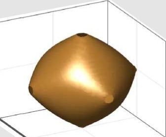
SCHRODI, APERIS, AND OPPENEER                                                                PHYSICAL REVIEW B 103, 064511 (2021)

extrapolation of normal-state properties, but also opens the         to very good accuracy. The paper is concluded in Sec. VI with
discussion of 3D systems, which has so far been elusive in           a brief discussion on related works, possible extensions to our
available literature. Our theory is based on a Holstein-like         theory, and potential future directions.
Hamiltonian, containing a nearest-neighbor tight-binding
model for the electron energies, an isotropic Einstein phonon                                   II. THEORY
mode, and isotropic electron-phonon scattering elements,
controlling the coupling strength in the system. We explore             We consider a phonon mode with frequency 0 and
here in detail the interplay of phonon softening, renormalized       electron-phonon coupling that is given by gq . Here the elec-
coupling strength, nesting properties, superconducting energy        tronic energies are modeled by a single band dispersion ξk ,
gap, and, eventually, the maximally possible transition              with k a BZ wave vector. By setting q = k − k we can write
temperature Tc .                                                     the Hamiltonian as
    Our theory takes the bare phonon frequency 0 , cou-
                                                                                                                          1
pling strength λ0 , and electron energies ξk as inputs. By                    H=       ξk k ρ̂3 k +
                                                                                           †
                                                                                                             h̄0 bq bq +
                                                                                                                    †

varying these quantities we pinpoint the renormalized cou-                          k                  q
                                                                                                                          2
pling strength and phonon softening (momentum dependent
decrease in magnitude) as key ingredients to how our self-                         +      gk−k uk−k k† ρ̂3 k .            (1)
                                                                                      k,k
consistent results change. Other crucially important aspects
for the interacting state are Fermi-surface (FS) nesting prop-       Above we use b†q and bq as bosonic creation and annihilation
erties of ξk and the size of the FS. There exists a critical value   operators, which determine the phonon displacement uq =
λ0 of the bare input coupling, at which the phonon energies         bq + b†−q . The electronic creation and annihilation operators
become negative, indicating a lattice instability. Another im-        †
                                                                     ck,σ and ck,σ are part of the Nambu spinor k† = (ck,↑
                                                                                                                        †
                                                                                                                            , c−k,↓ ),
portant value of λ0 marks the onset of superconductivity, λ    0.
                                                                     where σ ∈ {↑, ↓} is a spin label. The imaginary time τ depen-
In two dimensions we find an enhancement of both λ0 and λ      0   dent electron and phonon Green’s functions are, respectively,
with increased shallowness of ξk , which goes along with less
                                                                     given by
coherent nesting properties and a decrease in FS size. Notably,
we find that our model systems exhibit maximal supercon-                            Ĝk (τ ) = −Tτ k (τ ) ⊗ k† (0) ,           (2)
ducting transition temperatures Tc for an intermediate system
that is not very shallow, but also not ideally nested. For 3D                         Dq (τ ) = −Tτ uq (τ )uq (0) ,              (3)
systems the significance of FS nesting is weakened, such that
trends in λ0 , λ
                 0 , and maximum Tc are mainly dictated by the       where Tτ is the imaginary-time ordering operator. Both prop-
FS size. An exception to these tendencies is our most shallow        agators obey a Dyson equation in Matsubara space, reading
ξk considered in three dimensions, because in this particular
system nesting is exceptionally coherent due to the special                         Ĝk,m = Ĝ0k,m + Ĝ0k,m ˆ k,m Ĝk,m ,         (4)
role taken by the  point of the Brillouin zone (BZ).
    From here we proceed as follows: In Sec. II we introduce                          Dq,l = Dq,l
                                                                                              0
                                                                                                  + Dq,l
                                                                                                     0
                                                                                                              q,l Dq,l ,          (5)
the formalism and mathematical steps needed for deriving             where we make use of the notation f (k, iωm ) = fk,m
a self-consistent and full-bandwidth Eliashberg theory, that         with Matsubara frequencies ωm = π T (2m + 1) for generic
includes all lowest-order processes for electron and phonon          fermion functions f , and h(q, iql ) = hq,l for boson functions
self-energies. The terminology “full bandwidth” is used here         h, with ql = 2π T l. The above Eqs. (4) and (5) are solved
to stress that our equations are solved numerically by taking        for the dressed propagators as functions of the respective
into account the complete bandwidth of electron energies ξk ,        self-energies ˆ k,m and q,l :
rather than focusing on a narrow energy window around the                                       0 −1
Fermi level, as is common practice in Fermi-surface restricted                          Ĝ−1
                                                                                          k,m = Ĝk,m     − ˆ k,m ,              (6)
calculations. We provide some benchmark checks of our im-
                                                                                           −1      0 −1
plementation in the Appendix. We continue by introducing                                 Dq,l = Dq,l      − q,l .                (7)
electron dispersions in two and three dimensions (see Sec. III).
In particular, we define in both cases three different energies         The noninteracting Green’s functions are defined by
via varying the chemical potential, that differ in nesting and                         0 −1
                                                                                       Ĝk,m   = iωm ρ̂0 − ξk ρ̂3 ,            (8)
FS properties. In Sec. IV follows an exploration of phase
space, spanned by the different input parameters to our the-                                           −1
                                                                       0 −1          1           1                 1  2
ory. We discuss in detail the aspects of phonon softening,             Dq,l   =              −              =−          q + 20 ,
renormalization of electron-phonon coupling, and the onset of                      iql − 0    iql + 0             20 l
superconductivity, and try to unravel their complex interplay                                                                  (9)
by deriving approximate relations between them. In Sec. V the        where we use the Pauli matrices ρ̂i , i ∈ {0, 1, 2, 3}. The
subject is a closer discussion of the superconducting energy         electronic self-energy can be decomposed to the mass en-
gap as function of temperature, and consequently the transi-         hancement function Zk,m , chemical potential renormalization
tion temperatures, in two and three dimensions. Motivated by         k,m , and superconducting order parameter φk,m :
the precedent findings we propose a scaling law for the maxi-
mum transition temperature that models our numerical results               ˆ k,m = iωm (1 − Zk,m )ρ̂0 + k,m ρ̂3 + φk,m ρ̂1 .    (10)

                                                               064511-2
INFLUENCE OF PHONON RENORMALIZATION IN …                                                          PHYSICAL REVIEW B 103, 064511 (2021)

                                                                         the phonon self-energy as function of Zk,m , k,m , and φk,m :
                                                                                                 ωm Zk,m ωm+l Zk+q,m+l
                                                                             q,l = −2T |gq |
                                                                                             2

                                                                                               k,m
                                                                                                    k,m    k+q,m+l

                                                                                     ξk + k,m ξk+q + k+q,m+l       φk,m φk+q,m+l
                                                                                   −                             +                      .
                                                                                        k,m       k+q,m+l         k,m k+q,m+l
   FIG. 1. (a, b) Lowest-order Feynman diagram for the electron                                                                                   (21)
and phonon self-energy, respectively.
                                                                            The above equations are solved self-consistently in an it-
                                                                         erative manner: Assuming Zk,m , k,m , and φk,m are known
Together with Eq. (6) this leads to an inverse electron Green’s          from a previous iteration, we first calculate the phonon self-
function                                                                 energy via Eq. (21), by using also Eq. (13). With q,l at hand,
                                                                         and the bare phonon propagator in Eq. (9), we calculate the
      Ĝ−1
        k,m = iωm Zk,m ρ̂0 − (ξk + k,m )ρ̂3 − φk,m ρ̂1 ,        (11)    phonon Green’s function from Eq. (7), which then determines
                                                                         the electron-phonon interaction kernel Eq. (16). As final step
so that after matrix inversion we get                                    we solve for the mass renormalization, the chemical potential
                                                                         renormalization, and the gap function via Eqs. (18)–(20). This
  Ĝk,m = [iωm Zk,m ρ̂0 + (ξk + k,m )ρ̂3 + φk,m ρ̂1 ]−1
                                                       k,m , (12)        process is repeated until convergence is reached. From the
                                                                         results we can calculate the electron filling as
          k,m = (iωm Zk,m )2 − (ξk + k,m )2 − φk,m
                                                 2
                                                     .           (13)                                   ξk + k,m
                                                                                          n = 1 − 2T                   .           (22)
   In this paper we take into account all lowest-order pro-                                             k,m
                                                                                                              k,m
cesses in both the electron and phonon self-energies. The
corresponding Feynman diagrams are shown in Figs. 1(a) and                  The input to our theory is the electron dispersion ξk , the
1(b). By exploiting momentum and energy conservation in the              phonon frequency 0 , and the coupling λ0 , which can be
scattering processes we can translate the Feynman diagram for            expressed as
the electron self-energy into                                                                                  2N0
                                                                              λ0 = λk−k   k∈FS k ∈FS   =       |gk−k |2    k∈FS k ∈FS ,   (23)
                                                                                                              0
       ˆ k,m = −T      |gk−k |2 Dk−k ,m−m ρ̂3 Ĝk ,m ρ̂3 , (14)
                     k ,m                                              with N0 the density of states (DOS) at the FS. After solving
                                                                         self-consistently for the interacting state we have access to the
and for the phonon self-energy we obtain                                 renormalized coupling strength λq and frequencies q . These
                                                                        are, respectively, given as
            q,l = T |gq |
                          2
                              Tr{ρ̂3 Ĝk,m ρ̂3 Ĝk+q,m+l }.      (15)
                                                                                                λq = −N0 |gq |2 Dq,l=0 ,                          (24)
                                k,m

                                                                                              q =         20 + 20    q,l=0 ,                   (25)
   At this point it is convenient to define the electron-phonon
interaction kernel                                                       and it is convenient to define λ = λk−k k∈FS k ∈FS as a
                                                                         measure of the total coupling strength in the system. A nonva-
                          Vq,l = −|gq | Dq,l ,
                                         2
                                                                 (16)    nishing imaginary part of q marks a lattice instability.
                                                                             The theory presented here has been included in the UPP-
so that we can write Eq. (14) as
                                                                         SALA SUPERCONDUCTIVITY code (UppSC) [28–33], and we
                                                                        benchmark our implementation in the Appendix against ex-
             ˆ k,m = T     Vk−k ,m−m ρ̂3 Ĝk ,m ρ̂3 .        (17)    isting literature [8]. Momentum and frequency summations
                              k ,m                                     are carried out via efficient Fourier convolution techniques.
                                                                         For calculations in two dimensions (three dimensions) we use
Combining Eq. (17) with Eqs. (10) and (12) leads to the
                                                                         32 × 32 (32 × 32 × 32) points for the k and q grids. The
Eliashberg equations
                                                                         number of Matsubara frequencies is always chosen larger than
                        T                       ωm Zk ,m             2000. The equations given in our current paper are formulated
            Zk,m = 1 −              Vk−k ,m−m              ,   (18)    and solved in Matsubara space. Analogously, one can build
                       ωm k ,m                  k ,m
                                                                         up a theory as function of real frequencies, as has been done
                                           ξk + k ,m                in a recent work by Nosarzewski et al., where the authors
              k,m = T        Vk−k ,m−m                  ,     (19)
                       k ,m
                                               k ,m                   discuss the impact of phonon softening on various spectral
                                               φk ,m                  properties [34].
               φk,m = −T            Vk−k ,m−m          ,       (20)
                             k ,m
                                                 k ,m
                                                                                               III. MODEL SYSTEMS
from which the superconducting gap function can be defined                  In this section we introduce two kinds of electron disper-
as k,m = φk,m /Zk,m . Inserting Eq. (12) into Eq. (15) gives            sions that are employed in the rest of our paper. Starting in

                                                                   064511-3
SCHRODI, APERIS, AND OPPENEER PHYSICAL REVIEW B 103, 064511 (2021)
Turning now to the case of three spatial dimensions, we use
the electron energies
ξk = − 2t (1) cos(ki )
i=x,y,z
− 2t (2) cos(k j ) − μ. (27)
i=x,y,z j=x,y,z; j =i
Similarly as before we use an electronic bandwidth W =
1.5 eV and fix the hopping energies as t (1) = W/8, t (2) =
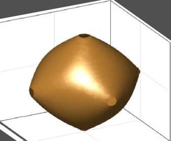
t (1) /4. We define three dispersions that are shown in Fig. 2(c)
along high-symmetry lines of the simple cubic BZ. The or-
ange (1), green (2), and purple (3) lines represent the choices
μ = −0.125, −0.625, and −1.075 eV, respectively. Again,
the resulting electron fillings are high, moderate, and low.
The FS shown in Fig. 2(d) is very large and resembles to a
good approximation an ideal Fermi gas. As the opposite case,
we have an extremely shallow energy dispersion reflected by
the tiny FS in Fig. 2(f). In Fig. 2(e) we show an intermediate
case. To avoid any possible misunderstandings, we note that
shallow bands are not to be confused with “flat bands” as the
latter host electrons with vanishing velocities and therefore
high electron DOS.
In the following we examine how the choice of electron
dispersion affects our self-consistent results of the Eliashberg
equations in two and three spatial dimensions. For simplifi-
cation we consider here isotropic electron-phonon scattering,
gq = g0 . As stated in Sec. II, the input to our Eliashberg equa-
FIG. 2. (a) Two-dimensional electron energies along high-
tions is the bare electron-phonon coupling λ0 , the electron
symmetry lines of the Brillouin zone. The purple, green, and orange
dispersion ξk , and the bare phonon frequency 0 . Since we
curves are found from Eq. (26) by choosing μ = −887.5, −437.5,
and 62.5 meV. (b) Fermi surfaces corresponding to panel (a), drawn
want to study trends with respect to those input parameters
in similar color code. (c) Three-dimensional electron dispersion ξk we need to pay special attention to the electron filling that
as calculated from Eq. (27) for different chemical potentials (orange, is calculated as function of the self-consistent results [see
μ = −0.125 eV; green, μ = −0.625 eV; purple, μ = −1.075 eV), Eq. (22)]. To be able to compare outcomes for different 0 ,
shown along high-symmetry lines. (d–f) Three-dimensional Fermi λ0 , and T we need to ensure that n stays constant, which
surfaces colored in correspondence to panel (c). In both two and three we achieve by introducing an additional chemical potential
dimensions we use labels (1), (2), and (3) to refer to the electron shift δμ, such that the input to the Eliashberg equations is
energies depicted by orange, green, and purple colors, respectively. ξk − δμ [35].
IV. PHONON SOFTENING, COUPLING,
two spatial dimensions we define the electron energies as AND SUPERCONDUCTING GAP
As a first step we want to understand how the input param-
ξk = −2t (1) [cos(kx ) + cos(ky )] eters influence our self-consistent results. For this purpose we
− 4t (2) cos(kx ) cos(ky ) − μ, (26) solve the Eliashberg equations in two dimensions as function
of λ0 at T = 20 K for various bare frequencies 0 . We show
where t (1) and t (2) are the nearest- and next-nearest-neighbor our results for dispersions (1), (2), and (3) of Fig. 2(a), respec-
hopping energies of our tight-binding model, and μ is the tively, in the first, second, and third column of Fig. 3 in the
chemical potential. For simplicity we assume here a tetragonal colors representing each ξk . In all of these columns we show
square-lattice structure in two dimensions, but our results results for different initial frequencies 0 with line styles as
hold qualitatively also for different symmetries. Whenever indicated in the legend of Fig. 3(g). The upper row shows the
referring to a 2D system, we choose t (1) = W/8 and t (2) = renormalized coupling strength as function of λ0 , where we
t (1) /4, where W = 1.5 eV is the electronic bandwidth. We test add as guide for the eye the case λ = λ0 as solid gray line.
three different examples for the choice of μ, the resulting The middle row shows the minimum renormalized phonon
dispersions along high-symmetry lines of the BZ are shown frequency, again as function of bare input coupling. The max-
in Fig. 2(a), while corresponding Fermi surfaces (same color imum superconducting gap, defined by = max k,m=0 , is
k∈BZ
code) are plotted in Fig. 2(b). The orange (1), green (2), and shown in the lower row.
purple (3) curves are, respectively, found using μ = 62.5, In Figs. 3(a)–3(c) we observe the well-known behavior
−437.5, and −887.5 meV, and correspond to high, moderate, of the renormalized coupling with increasing λ0 [5,8,10],
and low electron fillings. i.e., λ approaches a divergence, which we define to occur
064511-4
INFLUENCE OF PHONON RENORMALIZATION IN …                                                        PHYSICAL REVIEW B 103, 064511 (2021)

   FIG. 3. Results for the renormalized coupling strength λ (upper
row), minimum renormalized phonon frequency (middle row), and
maximum superconducting gap (lower row), calculated for our 2D
systems. Results shown in the first, second, and third column are
computed with the orange, green, and purple dispersion of Fig. 2(a),
respectively. Different line styles correspond to bare phonon frequen-
cies 0 as written in the legend of panel (g). The solid gray lines in
panels (a)–(c) refer to λ = λ0 .

                                                                             FIG. 4. Momentum dependent phonon frequencies, normalized
at λ0 . As is apparent in Figs. 3(d)–3(f), when λ0 → λ0 the            to the initial choice of 0 . Calculations were performed at T =
minimal phonon frequency vanishes, indicating a lattice in-              20 K. (a) Results for different bare couplings λ0 as written in the
stability. The average frequency on the other hand decreases             legend, computed for 0 = 100 meV and the orange dispersion (1)
approximately linearly with λ0 (not shown). Such tendencies              of Fig. 2(a). (b) Different colors correspond to the choice of 2D
towards a charge density wave instability occur at exchange              electron dispersion [compare Fig. 2(a)]. With λ0 = 0.2, the three
momenta following the most coherent nesting wave vector for              different line styles represent varying choices of bare frequency 0 as
the respective electron dispersion (see discussion below and             written in the legend. (c–e) Renormalized phonon frequencies along
Fig. 4). The slight increase in minimum phonon frequency,                high-symmetry lines of the BZ. Different colors correspond to 3D
seen for 0 = 200 meV in Fig. 3(f), can be interpreted as                electron energies as shown in Fig. 2(c). Bare couplings are chosen as
signature of a very nonadiabatic parameter choice, hence we              λ0 = 0.05, 0.1, and 0.15.
can expect that this feature disappears upon the inclusion of
vertex corrections. From Fig. 2(a) we know that the FS nesting
condition is met less accurately as we go from the orange (1)            superconducting state in connection with phonon renormal-
to the purple dispersion (3). The phonon self-energy exhibits            ization is provided in Sec. V.
less coherent contributions for the shallow energy band (3),                Including the back reaction of electrons on the phonon
which in turn renormalizes the phonon propagator to a smaller            spectrum, via the Feynman diagram shown in Fig. 1(b), leads
extent. For this reason we find increasing values of λ0 as we           to a decrease in the magnitude of frequencies, which is a
go from the first to the third column in Fig. 3. In line with this       well-known behavior commonly referred to as phonon soft-
observation we find the fastest decrease of minimum phonon               ening [36]. This phenomenon has been discussed especially
frequencies as function of λ0 in Fig. 3(d), and the slowest in           in context of the 2D Holstein model [4,5,12,15], and it marks
Fig. 3(f).                                                               tendencies of the system to develop a charge density wave
   From each of Figs. 3(g)–3(i) we observe that the supercon-            instability. The question of whether phonon softening is fa-
ducting gap opening with respect to λ0 depends on 0 . An                vorable for superconductivity or suppresses Tc is discussed in
increase in the initial phonon frequency reduces the minimal             further detail in Sec. V.
bare coupling strength needed for a finite superconducting                  To first show the general effect, let us consider the or-
gap. Further, comparing these three panels shows that the                ange dispersion (1) in Fig. 2(a) and a bare frequency 0 =
onset of superconductivity depends also on the electronic dis-           100 meV. After self-consistently solving the Eliashberg equa-
persion. This observation can again be understood in terms of            tions in two dimensions at T = 20 K, we calculate the
changed nesting conditions (see the discussion above). When              renormalized phonon spectrum via Eq. (25). In Fig. 4(a) we
considering the superconducting gap as function of λ (instead            plot our result for q /0 along high-symmetry lines of the
of λ0 ), the difference in the onset of  = 0 among results cal-         BZ for various coupling strengths as indicated in the legend.
culated for our three 2D electron dispersions becomes smaller.           In the limit of small λ0 (see blue curve), the renormalization
The onset of superconductivity with respect to λ0 is discussed           effects are relatively minor, i.e., q /0 stays close to unity
in more detail later in this section, and further analysis of the        throughout the BZ. The biggest phonon softening occurs at

                                                                   064511-5
SCHRODI, APERIS, AND OPPENEER                                                               PHYSICAL REVIEW B 103, 064511 (2021)

q (π , π ) because the FS is relatively well nested at this           wave vectors. Therefore we observe softer phonons around
exchange momentum. As we increase λ0 we confirm the                   in these results.
leading instability to be at (π , π ), since the smallest ratio of        In the discussion above we did identify FS nesting as
renormalized to bare frequencies is observed at this q [see           an important factor when considering phonon softening and
Fig. 4(a)]. Additionally, phonon softening occurs throughout          renormalized couplings in two dimensions. We now want to
the whole BZ, so we observe q < 0 ∀q for any finite λ0 .            explore this aspect also in 3D systems, using electron energies
     We can understand the observed decreases in q by                from Fig. 2(c). Fixing  = 100 meV, we solve the Eliashberg
                                                   q,l = −gq χq,l ,   equations for three different coupling strengths, λ0 = 0.05,
                                                            2 0
expressing the phonon self-energy as
where χq,l is the charge susceptibility [15]. Inserting
            0                                                         0.1, and 0.15, at T = 20 K. The corresponding results for the
                               √ gq = g0 gives q /0 =
into    Eq. (25) and using                                            phonon spectrum are shown in Figs. 4(c)–4(e), respectively.
√                                                                     Each of these panels contains results for all three electron fill-
   20 − 20 g20 χq,l=0
                   0
                        /0 = 1 − 2g20 χq,l=0
                                           0
                                                /0 . Therefore
                                                                      ings tested, where we adopt the color code of Figs. 2(c)–2(f).
the anisotropy in the renormalized frequencies comes solely
                                                                      The first observation is similar to the 2D case, i.e., the phonons
from the susceptibility, which in turn is dominated by
                                                                      become softer as we increase the coupling strength. This can
contributions due to FS nesting. In addition we note that
                                                                      be seen by comparing similarly colored curves among differ-
g20 /0 ∝ λ0 , therefore the phonon softening is expected to
                                                                      ent panels of Figs. 4(c)–4(e). Further it is apparent that the
increase with coupling strength, a trend confirmed by our
                                                                      phonon softening is generally less pronounced and coherent in
calculations shown in Fig. 4(a).
                                                                      three dimensions. The orange curves (1) in each panel show
     To further examine the influence of nesting on the phonon
                                                                      a relatively small tendency for phonon softening, while the
renormalization we test the three dispersions as shown in
                                                                      smallest q /0 are detected at M and R. Effects are even
Fig. 2(a). For each ξk we choose initial frequencies 0 =
                                                                      less prominent for the green lines (2) of each panel, where,
100, 150, or 200 meV and a coupling strength of λ0 = 0.2.
                                                                      for couplings up to λ0 = 0.15, q /0 stays relatively close
Our results for q /0 are plotted in Fig. 4(b), again as func-
                                                                      to unity throughout the BZ. For the smallest electron filling
tion of exchange momentum q along high-symmetry lines.
                                                                      (3), which is represented by purple lines in Figs. 4(c)–4(e), we
The color code is identical to Fig. 2(a), and we use varying
                                                                      find the results with highest anisotropy. Throughout most parts
line styles, as written in the legend, to show results computed
                                                                      of the BZ the phonon spectrum is to a good approximation
for different 0 .
                                                                      not renormalized, but q /0 decreases strongly around .
     As first observation we find that our results are to a good
                                                                      This behavior is qualitatively similar to the 2D case shown
approximation independent of the choice of bare phonon
                                                                      in Fig. 4(b), in contrast to the other curves shown here (green,
frequency. This is reflected in the fact that all three curves
                                                                      orange).
(different line styles) for any of the electron dispersions fall
                                                                          From the above discussion we learn that reduced nesting
almost precisely on top of each other. Therefore we conclude
                                                                      properties lead to less phonon softening in three dimensions,
that q /0 is a direct function of λ0 [see Fig. 4(a)] but not of
                                                                      compared to the 2D situation. However, very small electron
0 . This can √ be seen by expressing the above functional form
                                                                      fillings are an exception to this trend because we observe com-
as q /0 = 1 − λ0 χq,l=0 0
                               /N0 via Eq. (23). Notably, there is    parable results of q /0 in two and three dimensions. The
still an implicit dependence on 0 hidden in                          reason lies in the special role of the  point: When considering
                                                                     a spherical FS, q ∼ (0, 0, 0) is the only exchange vector with
            χq,l
             0
                 = −T          Tr[Ĝk,m ρ̂3 Ĝk+q,m+l ρ̂3 ]   (28)    which FS parts can be connected without dependence on the
                         k,m                                          angle of wave vector q, hence the susceptibility response in
                                                                      three dimensions can develop similarly coherent contributions
due to the self-consistency of our approach, which is why the         at  as in two dimensions.
curves are not precisely equivalent.                                      We now turn to a more detailed discussion of the renor-
    When comparing results computed for different electron            malized coupling strength λ, which, as we argue below,
fillings we find much bigger effects in the renormalized              does similarly as the phonon softening strongly depend on
phonon spectrum. Starting with the orange curves of Fig. 4(b),        FS nesting properties, and hence follows different trends in
we find the most pronounced phonon softening at q = (π , π ).         two and three dimensions. As stated before, the coupling
This case is already discussed above, and can be explained            diverges as we increase λ0 → λ0 , with λ0 marking a lattice
by well-satisfied nesting conditions at this wave vector. The         instability. Recalling the definition λ = λk−k k∈FS k ∈FS , we
green curves show larger values for q /0 , i.e., the renormal-      combine Eqs. (24) and (7) to write the momentum dependent
ization effects are less pronounced compared to results shown         coupling as
in orange. From the FS properties [see Fig. 2(b)], we know                                                           −1
that the exchange momentum is no longer close to M when                                             0
                                                                                      λq = N0 g20      +     q,l=0        ,        (29)
focusing on the green curve, rather q lies in between  and M                                       2
or X . This nesting property is directly translated into results
                                                                      where we used gq = g0 . With               = −g20 χq,l=0 and λ0 =
of Fig. 4(b), where the softest phonons are found along -M                                              q,l=0
                                                                      2g20 N0 /0 , we get
and X -. Turning now to the lowest electron filling, the purple
lines (3) in Figs. 4(b) and 2(a), the phonon frequencies q are                    λ = λk−k k∈FS k ∈FS
almost as large as their respective 0 , for q between M and
                                                                                                 λ0
X . Since the FS is a very small circle at the center of the BZ,                     =                                  .          (30)
it is not surprising that the susceptibility peaks only at small                          1 − λ0 χq,l=0 /N0 k∈FS k ∈FS

                                                                064511-6
INFLUENCE OF PHONON RENORMALIZATION IN … PHYSICAL REVIEW B 103, 064511 (2021)
FIG. 6. Bare coupling strength λ 0 , corresponding to the onset
FIG. 5. (a) Renormalized coupling strength as function of λ0 , of superconductivity, as function of input frequency 0 . Results are
calculated in two dimensions for 0 = 100 meV and T = 20 K. computed for T = 20 K, and the color code corresponds to Fig. 2.
Open circles represent our self-consistent results; solid lines are (a) Results for 2D electron dispersions. (b) Results for 3D electron
obtained from Eq. (31). (b) Critical couplings λ0 as function of 0 , dispersions.
shown for different dispersions in two and three dimensions. The
color code used here in panels (a) and (b) reflects the choice of
electron dispersion according to Figs. 2(a) and 2(c). Results obtained coherent, so that the resulting λ0 grows larger. Turning to
for two dimensions (three dimensions) are shown via solid (dashed) the dashed curves of Fig. 5(b) we find a different behavior.
lines. The values for λ0 are far less susceptible for changes in
the electron filling. Further, we find smaller values for bλ in
We model Eq. (30) by introducing the fitting function three dimensions than in two dimensions, which clarifies that
nesting in three dimensions is less important. An exception
λ0
λ ∼ aλ , (31) to this is the result drawn in purple, representing the most
1 − bλ λ0 shallow electron dispersion (3). As discussed in connection to
where aλ reflects the magnitude of the coupling, and bλ is a Figs. 4(c)–4(e), this stems from the special role of nesting at
measure of the influence due to χq,l=0 /N0 . Needless to say, q ∼ (0, 0, 0), which is developed to a larger extent in three
Eq. (31) is an approximation, since we neglect the momen- dimensions than in two dimensions. For this reason (large
tum dependence of the susceptibility. As mentioned earlier, value of bλ ) the purple dashed line not only falls below the
the renormalized coupling diverges at a critical choice λ0 of two other curves for 3D systems, but lies also lower than the
the bare coupling strength. We can find an estimate of this purple solid line obtained for the most shallow 2D electron
quantity from the denominator in Eq. (31), namely, when dispersion (3).
(1 − bλ λ0 ) → 0 we can write Note that the results of Fig. 5(b) are obtained by fitting
λ in the noncritical range of the input coupling, i.e., for λ0
1
λ0 . (32) significantly smaller than λ0 . Therefore the reported values of
bλ λ0 are to be interpreted as qualitative trends, and should not be
In Fig. 5(a) we show our self-consistent results for λ as taken as precise numbers. Performing a calculation at λ0 ∼ λ0
function of λ0 as open circles, for 0 = 100 meV, T = 20 K, is numerically very difficult, because the input ξk − δμ has to
and the three 2D electron dispersions of Fig. 2(a) (similar be gradually adjusted so as to keep the electron filling at the
color code). The fitted behavior as described in Eq. (31) is desired level. If, however, the interplay of δμ, 0 , and λ0 is
shown as solid lines for each data set. As is apparent from such that the input coupling is above the respective λ0 , the
this graph, the renormalized coupling strength can be modeled self-consistent Eliashberg loop never converges.
with the above functional form to a very good approximation. We end this section by looking into the bare coupling
Repeating the same procedure for 0 = 150 and 200 meV, strength λ 0 , at which the onset of superconductivity occurs,
and for all three 3D electron energies leads to the curves i.e., the smallest λ0 at which k,m = 0. As is apparent from
shown in Fig. 5(b), where we plot the critical bare coupling Fig. 3, λ 0 depends both on properties of the electron disper-
as function of input frequency. Solid (dashed) lines and open sion and on the phonon frequency, hence we want to examine
circles (crosses) represent trends in two dimensions (three this quantity closer in two and three dimensions. We choose
dimensions), while colors are again corresponding to the elec- phonon frequencies 0 as 70, 100, 150, or 200 meV, T =
tron dispersions in Figs. 2(a) and 2(c). 20 K and use electron energies from Figs. 2(a) and 2(c) to
From all curves of Fig. 5(b) we learn that λ0 is to first-order show computed results for λ 0 as function of 0 in Figs. 6(a)
approximation independent of the initial phonon frequency, and 6(b), for two and three dimensions, respectively. Open
which goes in line with observations from Fig. 4(b). Further, circles (crosses) represent our data, while solid (dashed) lines
our 2D results reflect the expected behavior with respect to are obtained by a linear fit of the 2D (3D) data. The color
nesting conditions: The orange dispersion (1) of Fig. 2(a) is code corresponds to choices of electron dispersion according
relatively well nested, therefore the susceptibility shows large to Fig. 2. For each of the curves, both in two and three di-
contributions that are reflected in the fitting constant bλ . Con- mensions, we observe a linear decrease in λ 0 with increasing
sequently, the critical input coupling [compare Eq. (32)] is a frequency. This stems from the fact that renormalized frequen-
small number. As we proceed to the green (2), and eventually cies q are growing with 0 , enhancing the tendencies of the
the purple (3) electron dispersion, the nesting becomes less system to form a superconducting state.
064511-7SCHRODI, APERIS, AND OPPENEER PHYSICAL REVIEW B 103, 064511 (2021)
be stabilized, so as to maximize the renormalized coupling
and critical temperature. Furthermore, each panel contains the
result for calculating (T ) without finite phonon self-energy,
i.e., setting q,l = 0, shown by the dotted cyan curves. For
each electron filling we compute these curves by setting 0 =
200 meV and matching Tc with the respective dot-dashed
result.
For Fig. 7(a) we take the parameter choices (0 , λ0 ) =
(100 meV, 0.205), (150 meV, 0.215), and (200 meV, 0.22).
The resulting critical temperatures lie between 26 and 65 K.
Next we turn to Fig. 7(b): The Fermi surface is smaller
than in the case before, but the electron band (2) is
not yet very shallow. We use (0 , λ0 ) = (100 meV, 0.34),
(150 meV, 0.41), and (200 meV, 0.42) for the solid, dashed,
and dot-dashed curves. As easily observed, Tc drastically
grows when compared to Fig. 7(a), with the largest critical
temperature almost reaching 200 K. When we finally go to
FIG. 7. Maximum superconducting gap as function of temper- the results for a shallow band (3) [Fig. 7(c)], Tc ranges be-
ature with color code corresponding to the electron dispersions of tween ≈80 and ≈110 K. Here the curves are produced by
Figs. 2(a) and 2(c). The different line styles represent the choices
choosing (0 , λ0 ) = (100 meV, 0.54), (150 meV, 0.53), and
of initial frequency 0 as written in the legends. For the size of
(200 meV, 0.55).
input couplings λ0 see main text. (a–c) Results for (T ) for the
The here observed results can be explained by an intuitive
2D electron systems. Each panel contains an example for (T )
shown by the cyan dotted curve, that is obtained by setting q,l = 0, picture: The dispersion corresponding to Fig. 7(a) exhibits the
0 = 200 meV, and matching Tc to the corresponding dot-dashed best nesting conditions, which leads to enhanced renormaliza-
curve. (d–f) Results for the 3D systems of Fig. 2(c), with coupling tion of the phonon propagator (see also Sec. IV). This means
strengths as described in the main text. that a substantial part of the available coupling in the system
is “used” for renormalizing the phonon frequency, leaving less
coupling available for Cooper pairing and therefore resulting
When comparing results for λ 0 with respect to shallow- in a reduction of and Tc . In the opposite limit of the shallow
ness and nesting, we find similar trends with those already band (3) [Fig. 7(c)], most of the initial coupling strength
observed in Figs. 4 and 5. In the 2D case [Fig. 6(a)], the is available to form the superconducting state, because the
orange dispersion (1) has the best nesting conditions, resulting nesting, and therefore the renormalization of the phonon spec-
in a large susceptibility at the nesting wave vector. This in trum, is comparatively minor. Consequently Tc is enhanced
turn leads to a relatively large renormalized coupling strength when comparing to Fig. 7(a). However, due to the shallowness
λ. By increasing shallowness of the electron energies, hence of the electron band (3) we face a reduced FS area, there-
considering the green (2) and purple (3) lines, we obtain de- fore the Tc ’s are larger than in Fig. 7(a), but not maximized.
creasing magnitudes of χq,l , which results in smaller coupling When comparing the results for 0 = 200 meV to the cyan
strengths. Hence, to achieve similar values of λ as in the well dotted curve, found for q,l = 0, in each panel we observe
nested case, λ0 has to be increased. For 3D systems nesting is larger values for /kB Tc when the phonon self-energy is fi-
generally less coherent, therefore the orange (1) and green (2)
nite. This comparison points towards stronger coupling when
curves in Fig. 6(b) show larger values for λ0 than in Fig. 6(a), including the self-consistent renormalization of the phonon
with similar reasoning. The very shallow ξk (3), represented
spectrum, which is rather intuitive when considering that the
by the purple line, is again the exception due to exhibiting
maximally possible λ0 < λ0 has been chosen here, leading
coherent nesting behavior at (0,0,0), which is why only small
to comparatively large values for the renormalized electron-
couplings are needed to induce superconductivity.
phonon coupling strength λ.
The results shown in Fig. 7(b) can be seen as example
V. CRITICAL TEMPERATURES of how to achieve the highest possible critical temperatures.
Let us now turn to the superconducting critical tempera- The electron dispersion (2) exhibits relatively bad nesting
ture Tc that can be determined by following the maximum conditions, while still not being in the limit of a very shallow
superconducting gap with T . We define Tc as the smallest band. For achieving a large magnitude of (and therefore
temperature at which vanishes and use the same electron Tc ) a substantial renormalized coupling λ is required, com-
dispersions as before [see Figs. 2(a) and 2(c)]. Starting in bined with a large FS. The system of Fig. 7(b) lies in an
two dimensions, we test the initial frequencies 0 being 100, ideal intermediate regime, where the balance between phonon
150, or 200 meV, which are represented in Figs. 7(a)–7(c) renormalization and electron band shallowness is kept. The
by solid, dashed, and dot-dashed lines, respectively. All pan- FS nesting condition is good enough for achieving a large
els show the maximum superconducting gap as function of λ, but not as ideal as in Fig. 7(a) so as to drive the system
temperature, with color code corresponding to the choice of towards a lattice instability before superconductivity can build
electron dispersion from Fig. 2(a). For each ξk and 0 we up. Additionally the FS size is sufficiently large, in contrast to
take the largest value of λ0 < λ0 for which a solution could Fig. 7(c), so as to boost values for Tc .
064511-8INFLUENCE OF PHONON RENORMALIZATION IN … PHYSICAL REVIEW B 103, 064511 (2021)
The above interpretation is the intuitive extension of results
well known for the approximation q,l = 0. If only the bare
phonon propagator is considered, one recovers the standard
BCS result, i.e., the superconducting critical temperature de-
pends on the phonon frequency and the FS size. An increase
in either of those quantities leads to a growing Tc . In contrast,
as soon as q,l is finite, the values of the maximum supercon-
ducting gap and critical temperature decrease to an extent that
depends only on the nesting conditions [compare Figs. 7(a)–
7(c)]. Therefore there should exist an ideal balance between
phonon renormalization and FS size, which maximizes the
critical temperature. FIG. 8. Influence of phonon renormalization on Tc in 2D and 3D
Let us now turn to 3D systems, taking electron energies systems. Open circles and crosses represent computed values for Tc
ξk from Fig. 2(c). The maximum superconducting gap as as function of renormalized frequency , where the color code of
function of temperature is shown in Figs. 7(d)–7(f), where we Fig. 2(a) (2D) and Fig. 2(c) (3D) is used for panels (a) and (b). The
test again three phonon frequencies for each electron filling couplings have been chosen close to the lattice instability. In the main
(see legend). Each curve is obtained by imposing a respective text we describe how to obtain the approximate upper bounds for Tc
input coupling λ0 that is close to the lattice instability. In as shown by the dashed lines.
Fig. 7(d) we plot our self-consistent solutions for (0 , λ0 ) =
(100 meV, 0.383), (150 meV, 0.4), and (200 meV, 0.42), us- (crosses). For finding these critical temperatures we choose
ing the orange electron dispersion (1) of Fig. 2(c). As initial frequencies 0 ∈ [50, 200] meV, and pick the largest
before we find a clear enhancement in the maximally al- λ0 < λ0 for which a solution can be stabilized.
lowed and Tc with increased phonon frequency. Results Our results show that the maximum Tc obtained here al-
for both maximum superconducting gap and critical tempera- ways increases as function of renormalized frequency =
ture become comparatively smaller in Fig. 7(e), (0 , λ0 ) = q q∈BZ for 2D systems. However, in three spatial di-
(100 meV, 0.31), (150 meV, 0.31), (200 meV, 0.33), where mensions this trend is not observed for our most shallow
the green dispersion of Fig. 2(c) is used. The reason for this dispersion (3), where Tc < 10 K for 150 meV. For mod-
trend is a decrease in FS size, combined with a less important eling the functional behavior found in Fig. 8, it is worthwhile
role of nesting properties in 3D systems. Finally, we show considering trends reported by other authors. In Ref. [9],
(T ) for the purple 3D dispersion (3) [see Fig. 2(c)], in Esterlis et al. proposed that Tcmax ∝ constitutes a reasonable
Fig. 7(f). Here we found no superconductivity for (0 , λ0 ) = upper bound for the critical temperature. However, our results
(200 meV, 0.15) and (150 meV, 0.12) down to 10 K. The gap do not appear linear in the renormalized phonon frequency,
size and Tc for (0 , λ0 ) = (100 meV, 0.1) are substantially which is why this scaling might be a too crude approximation.
smaller than in Figs. 7(d) and 7(f). These results can be Another proposal was made by Moussa and Cohen, stating
√
explained under the light of an extremely small FS of the that Tc ∝ 0 − 2 [37]. Imposing this form does indeed
max 2
purple electron dispersion (3). Additionally, large parts of lead to satisfying agreement with our data in two dimensions,
the available coupling are used for renormalizing the phonon but fails to capture the decrease in critical temperature ob-
spectrum, due to well-enhanced nesting conditions at q ∼ served for the purple line in Fig. 8(b). We find that the best fit
(0, 0, 0); see also discussions in Sec. IV. to our numerical data is given by the scaling expression
On a related note, our temperature-dependent results en-
able us to explicitly test the well-established practice of using kB Tcmax ∝ λ() 20 − 2 , (33)
the same phonon frequencies for all temperatures across the
superconducting phase transition. The phonon spectra are usu- which is shown as dashed lines in Fig. 8. As is apparent from
ally calculated in the normal state, i.e., without taking Cooper comparing our data with outcomes of Eq. (33), the functional
pairing into account, and afterwards used for describing the dependence in Fig. 8 is quite accurately captured. Especially
superconducting pair condensate at T < Tc . When consider- for 3D systems the inclusion of λ() is crucial to mimic the
ing q as function of T , we find that this is indeed a valid observed trends, while the functional dependence proposed in
approximation. For the model calculations done here, the Ref. [37] would suffice for the 2D cases.
changes are in the sub-meV range, with q slightly growing It is important to notice the difference between Eq. (33)
as T increases. This rather insignificant trend can be attributed and the more simplified scaling law of Ref. [37], since λ is
to thermal broadening, and can conveniently be neglected to not constant with respect to . To show this explicitly, we
very good approximation. can solve Eq. (25) for the zero-frequency phonon self-energy,
Above we have already encountered some aspects concern- yielding q,l=0 = (2q − 20 )/(20 ). We insert this expres-
ing the superconducting Tc , in both 2D and 3D systems. In sion into Eq. (29) and, as an approximation, replace q by ,
the following we propose a scaling of the critical temperature, so that
which can also serve as approximate upper bound. In Fig. 8
20
we show our maximally possible values for Tc as function kB Tcmax ∼ λ0 20 − 2 . (34)
of renormalized phonon frequency, adopting the color code 2
from Fig. 2. Our computed results for 2D and 3D systems Here it is furthermore worthwhile to note the functional de-
are, respectively, shown in Figs. 8(a) (open circles) and 8(b) pendence of the renormalized phonon frequency and bare
064511-9SCHRODI, APERIS, AND OPPENEER PHYSICAL REVIEW B 103, 064511 (2021)
coupling strength within our model, i.e., λ0 = λ0 (ξk , 0 ) and denoted λ in Ref. [8], which, again is not the same coupling
= (ξk , 0 ). strength as our λ0 corresponding to a lattice instability.
The interpretation of Eqs. (33) and (34) is rather intuitive: As mentioned before, various authors agree on the exis-
The highest possible value of Tc depends directly on the tence of a maximal coupling strength up to which Eliashberg
renormalized coupling strength in the system. Additionally, theory produces accurate outcomes. However, this aspect
well-developed phonon softening is advantageous for maxi- seems not to be understood completely yet. It has been
mizing the critical temperature, i.e., having 0 . These claimed that Migdal-Eliashberg theory breaks down at an
two effects are not decoupled from each other, since both input coupling λ0 0.4, which was concluded by consider-
depend on nesting properties and the FS size. For two di- ing a 2D Holstein model [7,8]. However, it is by no means
mensions we already observed the trends in Figs. 7(a)–7(c); clear whether the same limit exists in real materials, and in
the green curve in Fig. 8(a) represents the ideal compromise particular in 3D systems, as was implied, e.g., in Ref. [9]. Fur-
between magnitude of the FS (purple curve being suppressed thermore, other authors have arrived at deviating conclusions:
because the FS is too small) and nesting properties (or- In an early work by Marsiglio [4] good agreement between
ange curve being suppressed because phonon softening is QMC and Eliashberg theory was found regardless of coupling
too strong). Going from the orange to the green curve in strength, provided that the phonon renormalization is taken
Fig. 8(b) reflects the decrease of FS size (compare Fig. 2). self-consistently into account. We therefore conclude that the
The most shallow 3D system exhibits additionally coherent correct picture is currently still elusive, and want to stress
nesting at , so as to produce negative phonon frequencies again that results presented here are solely derived within
before superconductivity can fully develop. Summarizing, we Migdal’s approximation.
obtain numerically that the effect of phonon softening is in There are several aspects that go beyond the scope of the
general favorable for superconductivity, provided that the un- current paper, but are important to be considered in future
renormalized phonon frequency 0 is sufficiently large, such studies for gaining a better understanding of the formalism.
that the system is not developing a lattice instability before Examples of such extensions would be a nontrivial mo-
superconductivity can fully build up. mentum dependence in the electron-phonon coupling λq , or
replacing the Einstein phonon frequency 0 by a wave vector
and phonon branch ν dependent frequency ωq,ν . Especially
VI. CONCLUSIONS
a ν dependence would require a slight generalization of the
In this paper we have investigated the details of Eliash- equations used here. For simplicity, we have neglected any
berg theory including self-consistent phonon renormalization Coulomb repulsion, which should be included in our treat-
on a model basis. We worked out the similarities and dif- ment as well, ideally in a more exploratory manner than
ferences between 2D and 3D systems, identifying nesting just following the most commonly used practice of setting
properties and FS size as key aspects. From those follow μ = 0.1 [6]. Another major step further would be to extend
directly the trends for phonon softening, electron-phonon the vertex-corrected Eliashberg theory of Ref. [27] by a self-
renormalization, and the critical temperature. Our paper there- consistent phonon renormalization, which would then have to
fore constitutes an extensive overview of possible effects of be done by including up to the second-order processes in both
phonon renormalization in Eliashberg theory under Migdal’s electron and phonon self-energies.
approximation. Here we have solely considered optical phonon modes
Our calculations show that the maximally possible Tc in but it is worthwhile noting that potentially deviating results
two dimensions results from a delicate interplay between FS are to be expected for acoustic modes (characterized by
size and nesting properties. If the size of the FS is too small, ωq=(0,0),ν = 0). We have seen that the momentum dependent
no strongly increased values for Tc are found. On the other decrease in the magnitudes of optical phonon frequencies gen-
hand, very coherent nesting, which in our model is associated erally follows the nesting wave vector. However, for acoustic
with a big FS, drives the system too quickly towards a lattice frequencies this is not necessarily true, since the correspond-
instability with increasing coupling strength. Maximal values ing electron-phonon interaction λq,ν must then acquire a
for the critical temperature are therefore found in an interme- nontrivial momentum dependence, which has the constraint
diate regime. Comparable values for Tc when neglecting the λq=(0,0),ν = 0. Further, if a multibranch system is considered,
phonon renormalization are found for less strongly coupled not all branches are expected to be softened to the same ex-
systems. In three spatial dimensions, nesting, and therefore tent, which makes it rather difficult to predict the outcome of
the renormalization of the phonon spectrum, becomes less calculations similar to those we performed here for our model
coherent. Consistently we find that the magnitude of Tc is systems.
mainly dictated by the size of the FS. Additionally, we note that real materials have a degree
In Sec. IV we have shown that there exists an inherent of freedom not incorporated in our theory, which is struc-
bound λ0 on the maximal coupling strength, which is not to be tural transformations. A good example for discussing this
confused with critical values of λ0 in other works. Chubukov phenomenon is the high-temperature superconducting hy-
et al. use the notation λcr to describe the border of applicabil- drides [38,39]. These materials undergo one or more structural
ity of Eliashberg theory with respect to the electron-phonon phase transitions when subject to external pressure (see, e.g.,
coupling strength [7]. This border is found by comparing Ref. [40]). By calculating phonon spectra via density func-
outcomes from Eliashberg theory with QMC simulations in tional theory it is found that phonon softening is responsible
the normal state, so that for λ > λcr the two theories no longer for such structural reconfigurations, since nonstable phases
produce similar results. The same border of applicability is lead to imaginary frequencies at the nesting wave vector.
064511-10INFLUENCE OF PHONON RENORMALIZATION IN … PHYSICAL REVIEW B 103, 064511 (2021)
Therefore, for either optical or acoustic phonon modes, the
actual system adopts an atomic configuration that is stable
with respect to the lattice vibrations. Our analysis is valid for
testing different coupling strengths within one stable phase,
but not across such phase transitions.
ACKNOWLEDGMENTS
This work has been supported by the Swedish Research
Council, the Röntgen-Ångström Cluster, the Knut and Al-
ice Wallenberg Foundation (Grant No. 2015.0060), and the
Swedish National Infrastructure for Computing (SNIC).
APPENDIX: BENCHMARK CALCULATIONS
In the following we benchmark our formalism by compar-
ing it to existing literature to show that our implementation is
reliable and in agreement with other approaches. Specifically,
we compare our results with those of Ref. [8], where the
authors compare outcomes of quantum Monte Carlo calcula-
tions with results from Migdal-Eliashberg theory, computing
the charge density wave and superconducting susceptibilities.
The temperatures considered in this work exceed the phase
transition, i.e., the system is in the interacting but nonsuper-
conducting state. For their Eliashberg calculations the authors
include the electron and phonon lowest-order Feynman dia-
grams, similar to our present paper. The aim in this section is
to reproduce Figs. 3 and 4 published in Ref. [8].
Esterlis et al. [8] use a two-dimensional tight-binding
model with nearest- and next-nearest-neighbor hopping ener-
gies t and t . Their ratio is taken as t /t = −0.3. The electron
filling is fixed at n = 0.8. For both figures that we are inter- FIG. 9. (a–c) Imaginary part of the (11) element of the electron
self-energy as function of Matsubara frequencies. Results shown
ested in, the temperature is T = t/16, the adiabaticity ratio is
in panels (a), (b), and (c) are obtained for λ0 = 0.2, 0.4, and 0.5,
0 /EF = 0.1 (with EF the Fermi energy), and the coupling
respectively. Dashed curves are taken from Ref. [8], at FS angles
strength is chosen from λ0 ∈ {0.2, 0.4, 0.5}. The functional
as written in the legend. Blue and red solid lines correspond to our
form of their tight-binding approach reads results computed from Eq. (A2), where we show curves at those
ξk = −2t[cos(kx ) + cos(ky )] − 4t cos(kx ) cos(ky ) − μ FS momenta that produce the maximum (blue) and minimum (red)
(A1) magnitude for the self-energy. (d) Phonon frequencies, normalized
to the bare input 0 , along high-symmetry lines of the BZ. Different
for the electron energies [41]. The chemical potential μ has colors represent input couplings as written in the legend. For each λ0
to be adjusted so as to fix the electron filling at the cho- we show our results as solid lines, and curves taken from Ref. [8] are
sen value. In contrast to our theory presented here, Esterlis shown with dashed lines.
et al. [8] have focused on properties above Tc using a scalar
function (k, ωm ), while our Nambu formalism allows us
to directly access superconducting properties. We can make
contact between the two formulations by considering only the phonon frequency spectrum of Ref. [8], which can be obtained
(11) matrix element of ˆ k,m : with the same set of parameters as described above. We show
(11) our results for λ0 = 0.2, 0.4, and 0.5 in Fig. 9(d) via solid
−Im ˆ k,m = ωm (Zk,m − 1), (A2)
brown, gray, and purple lines, respectively. As before, we
which is equivalent to the scalar self-energy of Ref. [8]. find good agreement with results by Esterlis et al., plotted as
In Figs. 9(a)–9(c) we show our results for Eq. (A2) as solid dashed curves in similar color code.
lines in all three panels, corresponding to different choices of The small deviations between our results and those of
(11)
λ0 . We plot −Im ˆ k,m at those FS momenta, that produce the Ref. [8] observed in Fig. 9 can be likely attributed to dif-
maximal (blue curve) and minimal (red curve) magnitude of ferent choices for the momentum grid size and number of
the result. As comparison we extracted results from Ref. [8] Matsubara frequencies. Further, potential differences can arise
at two different FS angles (see the orange and green dashed from numerical details of the implementation, e.g., the way of
lines). It is directly apparent that the curves coincide to a very performing the momentum and energy integrals, or how the
good degree. Next, we attempt to reproduce the renormalized aspect of electron filling is handled.
064511-11You can also read