Reconstructing Building Interiors from Images
←
→
Page content transcription
If your browser does not render page correctly, please read the page content below
Reconstructing Building Interiors from Images

      Yasutaka Furukawa, Brian Curless, Steven M. Seitz                                     Richard Szeliski
           University of Washington, Seattle, USA                                 Microsoft Research, Redmond, USA
         {furukawa,curless,seitz}@cs.washington.edu                                       szeliski@microsoft.com

                           Abstract
   This paper proposes a fully automated 3D reconstruc-
tion and visualization system for architectural scenes (in-
teriors and exteriors). The reconstruction of indoor envi-
ronments from photographs is particularly challenging due
to texture-poor planar surfaces such as uniformly-painted
walls. Our system first uses structure-from-motion, multi-               Figure 1: Floor plan and photograph of a house interior.
view stereo, and a stereo algorithm specifically designed for
Manhattan-world scenes (scenes consisting predominantly                 rooms, with only a small subset visible in each photo. Third,
of piece-wise planar surfaces with dominant directions) to              capturing an entire house interior poses a significant scala-
calibrate the cameras and to recover initial 3D geometry in             bility challenge, particularly given the prevalence of thin
the form of oriented points and depth maps. Next, the initial           structures such as doors, walls, and tables that demand high
geometry is fused into a 3D model with a novel depth-map                resolution relative to the scale of the scene. These factors
integration algorithm that, again, makes use of Manhattan-              pose significant problems for multi-view stereo methods
world assumptions and produces simplified 3D models. Fi-                (MVS) that perform relatively poorly for interior scenes.
nally, the system enables the exploration of reconstructed                  Our goal is a fully automatic system capable of recon-
environments with an interactive, image-based 3D viewer.                structing and visualizing an entire house interior. The visu-
We demonstrate results on several challenging datasets, in-             alization should be compelling and photorealistic. Taking
cluding a 3D reconstruction and image-based walk-through                inspiration from image-based rendering approaches [7, 11],
of an entire floor of a house, the first result of this kind from       we seek to reconstruct simple models, reminiscent of the
an automated computer vision system.                                    floor plan in Fig. 1, which can then be rendered with the
                                                                        input images to hallucinate visual detail and parallax not
                                                                        actually present in the reconstruction. Our approach builds
1. Introduction                                                         on a number of existing techniques to achieve this goal. In-
    3D reconstruction and visualization of architectural                deed, our primary contribution is the design of a system that
scenes is an increasingly important research problem, with              significantly advances the state of the art for automatically
large scale efforts underway to recover models of cities at a           reconstructing and visualizing interiors.
global scale (e.g., Google Earth, Virtual Earth). While user-               We start with the observation that, as illustrated in Fig. 1,
assisted approaches have long proven effective for facade               architectural scenes often have strong planar arrangements,
modeling [7, 16, 24, 19], an exciting new development is                and their floor plans, though sometimes irregular, are usu-
the emergence of fully-automated approaches for the recon-              ally highly structured, typically with walls (and floors and
struction of urban outdoor environments both from ground-               ceilings) aligned with one of three orthogonal axes. Ac-
level and aerial images [5, 17, 26].                                    cordingly, we invoke the Manhattan-world assumption [6],
    Unfortunately, if you walk inside your home and take                which states that all surfaces are aligned with three dom-
photographs, generating a compelling 3D reconstruction                  inant directions, typically corresponding to the X, Y, and
and visualization becomes much more difficult. In con-                  Z axes. Clearly, restricting some surfaces to these orien-
trast to building exteriors, the reconstruction of interiors is         tations will help recover large-scale structures such as the
complicated by a number of factors. First, interiors are of-            walls aligned with the floor plan. We take this to an ex-
ten dominated by painted walls and other texture-poor sur-              treme by requiring that all reconstructed surfaces have this
faces. Second, visibility reasoning is more complicated for             restriction; even “lumpy” objects will be reconstructed as a
interiors, as a floor plan may contain several interconnected           union of box-like structures. These structures then serve as

                                                                    1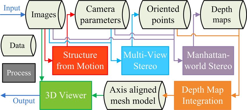
geometric proxies for image-based rendering (IBR).
    Given a set of images of a scene, we first use structure-
from-motion [20] and multi-view stereo (MVS) [9] soft-
ware to calibrate the cameras and obtain an initial 3D recon-
struction in the form of oriented 3D points. Next, a stereo
algorithm designed specifically for Manhattan-world scenes
is used to generate axis-aligned depth maps for the input im-
ages [8]. Then, the depth maps and MVS points are merged
into a final 3D model using a novel depth-map integration
algorithm that: (1) poses the reconstruction problem as a                         Figure 2: 3D reconstruction and visualization system for
volumetric MRF on a binary voxel grid, (2) solves it us-                          architectural scenes. See text for details.
ing graph-cuts, and (3) extracts a simplified, axis-aligned
mesh model. Finally, the system provides virtual explo-                           3D space of interest, perform a volumetric reconstruction
ration of reconstructed environments with an interactive,                         on voxels, and use marching cubes [15] to extract a mesh
image-based 3D viewer. To our knowledge, our system is                            model. However, these techniques produce extremely de-
the first fully automated computer vision system to recon-                        tailed and complex 3D models; operating on the scale of a
struct and enable the walkthrough of an entire floor of a                         full house interior poses a major challenge. We instead fo-
house.                                                                            cus on extracting very simple 3D models that exploit known
                                                                                  properties of architectural scenes. Our 3D viewer uses a
1.1. Related Work                                                                 reconstructed mesh model as a geometric proxy for view-
    Automated 3D reconstruction algorithms can be roughly                         dependent texture mapping as used in [7, 21] and Façade.
classified as either model-based approaches that reconstruct                      Other IBR methods that leverage a geometric proxy, e.g.,
scenes composed of simple geometric primitives [5, 7, 16,                         unstructured lumigraphs [4], could be used instead.
24], or dense approaches where the objective is to capture
fine details without strong priors.                                               2. System Pipeline
    Multi-view stereo (MVS) is one of the most successful                             This section describes the overall pipeline of our pro-
dense approaches and produces models whose accuracy ri-                           posed 3D reconstruction and visualization system illus-
vals laser range scanners [18]. However, MVS requires                             trated in Fig. 2. Our system consists of four steps.
texture and thus architectural scenes pose a problem due
to the prevalence of texture-poor, painted walls. Further-                        Camera Calibration and Initial Reconstruction
more, MVS focuses on producing high resolution 3D mod-                            Given a set of images of a scene, the first step is to com-
els, which we argue is overkill for architecture, which con-                      pute camera viewpoints and parameters; we use the Bundler
sist largely of flat walls. While it is possible to simplify                      Structure from Motion (SfM) package for this purpose [20].
MVS models of architecture as a post-process, we show                             Next, multi-view stereo (MVS) software PMVS [9], which
that this approach yields disappointing results. Model-                           is also publicly available, is used to reconstruct dense 3D
based approaches, on the other hand, incorporate scene-                           oriented points, where each oriented point is associated with
specific constraints to improve the robustness of reconstruc-                     its 3D location, surface normal, and a set of visible images.
tion. Notable examples include Cornelis et al. [5], who re-                       Manhattan-world Stereo
constructed entire city streets from car-mounted video by                         Due to lack of texture and other challenges, MVS produces
restricting the geometry to vertical ruled surfaces.1 Aerial                      incomplete models for most architectural scenes. There-
images are used for reconstructing building models in [26],                       fore, some form of interpolation is needed to compute a full
where the system uses a height field, a rough building mask,                      model from the oriented points reconstructed in the previ-
and 3D lines to segment out buildings from images and to                          ous step. For this purpose, our system uses a stereo algo-
reconstruct roof shapes. Their system produces very im-                           rithm proposed by Furukawa et al. [8], which exploits the
pressive results for outdoor environments, but it relies heav-                    Manhattan-world assumption: surfaces are piece-wise pla-
ily on obtaining dense, accurate stereo (more problematic                         nar and aligned with three dominant directions. The out-
for interiors, as we demonstrate).                                                put of this algorithm is a complete depth map for each in-
    Our depth map integration approach is similar to sev-                         put image, and the algorithm operates as follows. First, it
eral existing MVS approaches [13, 25], where they first en-                       identifies three dominant orientations in the scene from the
code depth map information into a voxel grid covering the                         surface normal estimates associated with MVS points. Sec-
    1 Pollefeys et al. also reconstruct street-side views while exploiting cer-   ond, it generates a set of candidate planes along each dom-
tain structural information, but their system is a dense approach producing       inant axis on which most of the geometry lies by extracting
high resolution models.                                                           peaks from the density of MVS points projected onto the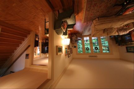
axis. Lastly, it recovers a depth map for an input image by                    v- pv                              depth map
                                                                                                   pv                 Di        S i(v)=1
assigning one of the candidate planes to each pixel, which
                                                                                                                   interior
is posed as a Markov random field (MRF) and solved with                                                             space
graph cuts [3]. Refer to [8] for more details.2                                v
                                                                                                                   margin
                                                                                                       Ω(pv)
Axis-aligned Depth Map Integration                                                   d i(v)
                                                                                                                    exterior
                                                                                                                     space                 T i(v)=1
Our final reconstruction step is to merge axis-aligned depth                                                   optical center
maps into a 3D mesh model. Details are given in Section 3.                         (a)           (b)                             (c)

3D Viewer                                                                  Figure 3: (a) Given a voxel v, pv denotes the pixel on depth
Given a 3D model of a scene, the system allows users to                    map Di that is closest to the image projection of v, while v̄
explore the reconstructed environment using an interactive                 is the voxel immediately behind pv . (b) Ω(pv ) denotes a set
image-based 3D viewer. As mentioned in the introduc-                       of voxels that is in front of p. (c) Each depth map votes for
tion, a reconstructed model is used as a geometric proxy                   interior and exterior assignments.
for view-dependent texture mapping as in [7, 21], where
two images are used for alpha-blending in every frame, with                of the input cameras. The resolution of the voxel grid is
the blending weights being inversely proportional to the dis-              determined by a user-controlled parameter Nr that specifies
tances between the current viewpoint and the optical centers               the number of voxels along the longest dominant direction.
of the cameras used for texture-mapping. The viewpoint                        Given a depth map Di and a voxel v, pv is used to denote
can be controlled in the following two navigation modes.                   a pixel on Di (and the corresponding 3D point on Di inter-
In the first mode, a user simply navigates through the in-                 changeably) that is closest to the image projection of the
put images in a pre-specified order (e.g., the order in which              voxel center, and v̄ denotes the voxel that is immediately
the pictures were taken). In the second mode, a user has                   behind pv on the opposite side from the camera (Fig. 3a–
a restricted free-form 6-DOF navigation: A viewpoint can                   b). Ω(pv ) denotes the set of voxels intersected by the ray
move freely in 3D space, while the viewer keeps track of                   from pv to the optical center of Di . Finally, di (v) is used to
distances to all the cameras. Whenever the closest camera                  represent the depth value of v with respect to Di .
changes, the viewpoint automatically moves to that camera
with rotational motion to align viewing positions and direc-               3.2. Volumetric Reconstruction
tions, after which a user has free control over the viewpoint                 Following recent work in MVS surface reconstruc-
again. In this mode, since we have a full 3D model of an en-               tion [13, 23], we set each voxel to have a binary label, either
vironment, the viewer performs collision detection to avoid,               interior or exterior (int or ext). 4 We use graph-cuts [3] to
e.g., passing through walls.                                               minimize an objective of the form:
                                                                                      X                     X
3. Axis-aligned Depth Map Integration                                           F =        F1 (lv ) + λ1            F2 (lv , lu ),     (1)
   Recent MVS algorithms have shown that first recon-                                     v∈V                    v∈V,u∈N (v)
structing depth maps and then merging them into a surface
can yield competitive reconstructions [18]. We follow this                 where lv is the label assigned to voxel v, N (v) denotes
approach, starting from Manhattan-world depth maps [8].                    neighboring voxels, and λ1 controls the relative effect of
We formulate an objective over a cost volume with binary                   the unary and binary functions, F1 and F2 , respectively.
labels and optimize with graph-cuts. In this section, we                      In previous formulations, F2 (lv , lu ) has encoded the ob-
describe our formulation, surface extraction algorithm, and                servations of the surface location. Evidence (from photo-
several enhancements suitable for architectural scenes.                    consistency or extracted depths) that a surface should ap-
                                                                           pear between two voxels can be used to relax the cost of
3.1. Problem Setup and Notation                                            transitioning from interior to exterior. This term implicitly
    The input to the volumetric reconstruction step is a                   seeks a weighted minimal surface, a kind of regularization
set of depths maps {D1 , D2 , · · · } containing axis-aligned              that favors constructing tight surfaces, particularly where
surfaces reconstructed by a Manhattan-world stereo algo-                   no data otherwise drives the surface. By contrast, F1 has
rithm [8], and the associated three dominant axes of the                   either been an inflating term [23]—a small constant penal-
scene.3 We first compute the smallest axis-aligned bound-                  izing empty voxels, to avoid the degenerate solution of no
ing box that contains all the depth maps and optical centers               surface at all—or has been informed by visibility informa-
                                                                           tion derived from depth maps [13]. When implementing the
   2 For the gallery dataset, which is the most complicated, we also en-

force depthmaps to be inside the smallest axis-aligned bounding box that   algorithm is independent of the orthogonality of the axes. Here, we as-
contains MVS points.                                                       sume that the axes form orthogonal bases for simplicity.
   3 Extracted dominant axes may not be perfectly orthogonal to each          4 Interior and exterior voxels are also referred to as full and empty, re-

other. In that case, our voxel grid would be skewed, but the rest of the   spectively.
graph, a 26-neighborhood around each voxel is preferred to twice the voxel resolution (γ = 2µ) in our experiments.
help recover oriented surfaces, although 6-neighborhoods We could now set F1 (lv = int) = E(v) and F1 (lv =
(neighbors along coordinate axes) are often used to reduce ext) = I(v). In practice, however, we have found that
memory footprint and accelerate computation [23]. depth maps generated by Manhattan-world stereo can occa-
Our formulation departs from these approaches in the sionally go quite astray from the true surface. Implicit in our
following ways. First, to favor simple surfaces, we use the voting scheme (and made explicit in [13]) is the assumption
regularizing effect of minimal surface area as our smooth- that the certainty (and thus weight) of visibility information
ness term by setting F2 (lv , lu ) = δ(lv = lu ). Note that this provided by a pixel in a depth map depends only on the re-
term does not depend at all on the observations. Instead the constructed depth at that pixel. However, the depths at some
observations—depth maps in our case—are used to drive pixels are inconsistent with other depth maps, and should be
the unary term F1 , providing evidence for the emptiness or down-weighted. In particular, we set the label costs to:
fullness of voxels based on visibility.5 In addition, we con-
sciously employ a 6-neighborhood around voxels and add a F1 (lv = int) = ΣN i i i
i=1 ω (pv )ψ (v)E (v),
c
(3)
shrinkage term (see below) to the energy that penalizes full F1 (lv = ext) = ΣN i i
i=1 ω (pv )I (v).
c
(4)
voxels. This simple combination leads to small numbers of
clean, sharp corners in areas where no observations drive where ω i (pv ) measures the confidence of the depth at
the surface, which is a desirable property for reconstruct- pixel pv based on consistency with other depth maps, and
ing architectural interiors.6 The minimum area and volume ψ i (v) is a correction term that balances volumetric costs
terms might seem to drive toward an empty volume solu- against surface hcosts (more on this below). We define i
ω i (pv ) = exp 81 I(v̄) − λ2 E(v̄) + v0 ∈Ω(pv ) I(v 0 ) .
P
tion. However, our Manhattan-world depth maps are quite
dense, providing ample data to avoid such a collapse. The first term I(v̄) in the exponent is the number of depth
Next we describe our definition of the unary term F1 (lv ). maps that pass through the same location pv , and hence,
Similar to [13], we base this term on the visibility infor- agree with its depth. The next terms measure conflicts (and
mation implied by the depth maps. We employ an occu- are thus subtracted from the number of agreements). The
pancy voting scheme. If the depth maps vote that a voxel first conflict term is the number of depth maps whose exte-
should be empty (due to visibility), we assign a high cost to rior space, which should be empty, contains pv . The second
F1 (lv = int). If a voxel is just behind reconstructed depths conflict term is the number of times the space from pv to
in many views, it is likely occupied, and a high cost should its depth map’s center of projection, which again should be
be assigned to F1 (lv = ext). We can accumulate votes empty, contains depths observed by other cameras. Intu-
for eachPvoxel by summing overP the depth maps as follows: itively, the weight ω i (pv ) becomes smaller when the mea-
Nc Nc
I(v) = i=1 I i (v), E(v) = i=1 E i (v). sure of agreement I(v̄) is small or that of conflict E(v̄) and
i i
I (v) and E (v) are the amount of evidence for being inte- I(v 0 ) is large. Values chosen for λ2 are given in Table. 1.
rior and exterior, respectively, based on a single depth map Finally, ψ i (v) reduces the effects of exterior information
Di , and Nc is the number of input cameras. We set I i (v) to i
E (v) exponentially based on the h distance from the i depth
be 1 where v should be interior, that is, immediately behind map to v: ψ i (v) = min 1, exp − d
i
(pv )−di (v)−γ
.
8µ
Di , and E i (v) to be 1 where v should be exterior, that is, in
front of Di (see Fig. 3c): The motivation for this scaling term is that F1 (lv = int)
and F1 (lv = ext) as defined in Equation 4, would have dif-
I i (v) = 1 if 0 < di (v) − di (pv ) ≤ µ, (2) ferent units otherwise: The interior evidence lies immedi-
E (v) = 1 if 0 < di (v) and di (v) − di (pv ) ≤ −γ.
i ately behind depth maps, and hence, covers a 2D manifold,
while exterior evidence covers a 3D space in front of the
Note that I i (v) and E i (v) are 0 in all the other cases, and depth map. The unit difference is particularly problematic
γ is a margin to allow errors in depth maps, which is set to when input depth maps contain large errors.
5 Hernández et al. [13] use both a data-dependent binary term, and Minimum-volume solution: We have observed that the
visibility-driven (thus also data-dependent) unary term. We encode the global minimum of the energy function (1) is often not
entire data contribution in the latter. unique, because the smoothness term F2 alone is ambigu-
6 One could certainly imagine more direct schemes for encouraging
ous where there is no data information. Figure 4 illustrates
simple, axis-aligned reconstructions, e.g., directly computing a final 3D an example (in 2D) of a depth map and its corresponding
model from MVS points without the Manhattan-world stereo step. In-
deed, we experimented with smoothness penalties based on higher-order minimum-volume and maximum-volume solutions. As we
cliques that prefer axis-aligned piece-wise planar surfaces. However, the use a 6-neighborhood in 3D, these solutions have the same
energy terms became non-submodular. We tested several approximation amount of energy; i.e., the area is measured in voxel faces,
algorithms such as quadratic pseudo-boolean optimization (QPBO) [12]
and a submodular-supermodular procedure, but the optimizations settled
and a monotonic, jagged path has just as many boundary
in undesirable local minima. In practice, the simple smoothness penalty faces as two axis-aligned planes that cleanly form a corner.
F2 described above produces satisfactory results. Indeed, there is a family of surfaces between these two thatDepth map evidence Min volume solution Max volume solution grid slice
connected components
Constrained delaunay triangulation
surface boundary surface boundary
(smoothness penalty) (smoothness penalty) Figure 5: Delaunay triangulation is used for each con-
depth map interior exterior margin nected component on each grid slice to triangulate the re-
constructed volume.
Figure 4: The global minimum of our energy function (1)
is usually not unique. We choose the minimum-volume sur- connected component, visiting each exactly once.
face as the solution, which tends to be less jagged. Yel-
low lines in the right two figures represent the amount of 3.4. Enhancements
smoothness penalties; the total penalties are equal in these We now describe several optimizations and implementa-
two cases. tion details suited to architectural reconstruction.
Grid pruning: When reconstructing large-scale scenes,
have the same energy. In general, the minimum-volume sur- we adapt the voxel resolution spatially according to the in-
face is smoother, because it can cut, without penalty along put depth maps. This adaptation accelerates the reconstruc-
straight paths into regions that are not observed. By con- tion, reduce memory footprint, and provide a level-of-detail
trast, the maximum volume surface tends to be jagged, as control. Octree partitioning of space is one possible adap-
it must conform to the boundary (between blue and white tation strategy [13]. However, this approach does not take
in the figure) constrained by visibility. Surfaces between advantage of the fact that floor plans often have large, un-
the minimum and maximum will also be more jagged than evenly spaced planes, some of which align with multiple
the minimum solution. In practice, we add a small penalty disconnected walls. Instead, we take a simple pruning ap-
(10−6 ) to F1 (lv = int), and find the solution with the proach, removing voxel slices that are not supported by the
minimum volume. It is straightforward to show that these depth maps. In particular, given a pixel in a depth map, we
same arguments do not hold for 26-neighborhoods, where define it to be a grid pixel if it corresponds to a corner or an
the minimum volume solution will not in general result in edge of the depth map, i.e., if its candidate plane assigned
two planes meeting at a corner in cases such as the one de- by the Manhattan-world stereo algorithm is different from
scribed here. that of a neighboring pixel. Intuitively, grid pixels occur
most often at scene corners and edges, and hence, we want
3.3. Mesh Extraction with Sub-voxel Refinement grid slices to pass through them. So, for each grid slice, we
After using graph cuts [3] to find the optimal label as- count the number of grid pixels (their 3D locations) that are
signment, we triangulate the boundary between interior and within µ/2 distance of the slice and prune the slice away if
exterior voxels to extract a mesh model, where the bound- the count is less than threshold λ3 . We modify the prob-
ary is defined as a set of voxel faces whose incident vox- lem formulation to account for the larger voxel cells, which
els have different labels. We also refine vertex positions up implicitly contain the original fine resolution cells, using
to sub-voxel accuracy while keeping the axis-aligned struc- a procedure known as contraction [12]. See Tables 1 and 2
ture. More concretely, for each (axis-aligned) slice of the for the values of λ3 and the amount of speed-up achieved by
voxel grid, we identify a set of voxel faces that belong to the this procedure. Fig. 6 shows how changing the value of λ3
surface boundary. For every connected component C, we can be used to control model complexity; raising the thresh-
then create a constrained delaunay triangulation [2], where old removes small scale structure to create simpler models.
the boundaries of the component (including any holes) are Ground plane determination: Ground planes may not
constrained to be part of the triangulation (see Fig. 5). After be clearly visible in the input images (e.g., when photos are
repeating this for all slices, the result is a sparsely triangu- taken by pointing the camera horizontally), and hence, are
lated mesh with faces and edges aligned with the voxel grid. not reconstructed well in the depth maps. In these cases,
Next, we compute a sub-voxel offset along the normal di- Manhattan-world stereo may extrapolate surfaces below the
rection to each component C by: (1) collecting MVS points ground plane, thus increasing the bounding box of the vol-
that are within 1.5µ of C and have a compatible normal ume and reconstructing surfaces below ground. We tighten
(i.e., within 45 degrees of C’s normal), and (2) computing the bounding volume to match the ground plane as follows.
the (signed) distance to the centroid of the collected MVS Among the six (directed) dominant directions, the upwards
points. The vertices of C are then shifted by this distance vertical axis is determined by the one that is compatible (an-
in C’s normal direction. We repeat this process for every gle difference is less than 45 degrees) with the most num-kitchen hall house gallery MWS step is currently the bottleneck of the system, where
# images (Nc) 22 97 148 492 it computes depth maps for all the input images. To acceler-
image res [pixel] 3M 3M 2M 2M ate this step, each depth map could be computed in parallel
# voxels (Nr) 128 150 256 512 (a few minutes per depth map).
# faces 1364 3344 8196 8302
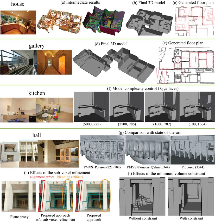
Figure 6a shows intermediate reconstructions, in partic-
voxel num ratio 0.15 0.036 0.071 0.0052
ular, MVS points and axis-aligned depth maps for the house
λ1 1 1 1 1
dataset. The final 3D models are shown in Figure 6bd for
λ2 1/16 1/16 1/16 1/16
house and gallery (see the project website [1] for more re-
λ3 100 100 10000 15000
sults and better visualization on all the datasets). Note that
run time (SfM) 13 76 92 716
MVS points are sparse in many places, and depth maps are
run time (MVS) 38 158 147 130
fairly noisy. Nonetheless, our algorithm has successfully
run time (MWS) 39.6 281.3 843.6 5677.4
run time (DI) 0.4 0.4 3.6 22.4
reconstructed extremely simple models while discovering
large-scale structure such as ground planes or vertical walls
Table 1: Characteristics of datasets. See text for details. each of which is represented by a single or a few planar
surfaces. In Figure 6ce, we generate floor plan images of
ber of camera up-vectors. Then, for each horizontal volume the house and the gallery datasets (red) by projecting ver-
slice (of the original volume), we count the number of asso- tical surfaces of the model to the horizontal plane, where a
ciated grid pixels and compute the average of the non-zero pixel intensity represents the amount of projected surface.
counts. The ground plane is determined to be the bottom- We manually align them with actual floor plans to evaluate
most slice with a count greater than this average, and the the accuracy. They are fairly consistent, though there is a
bounding volume is then restricted to go no lower than this small amount of global warping, probably due to calibration
ground plane. (For interiors, a ceiling plane could be needed (SfM) errors. It is also worth pointing out that walls recon-
as well, though this proved unnecessary in our examples.) structed in the middle of house and gallery are extremely
Boundary filling: After the volumetric label optimiza- thin, difficult for general MVS algorithms to recover. Our
tion but before the surface extraction step, we mark all the system is capable of reconstructing small objects in a scene
voxels at the boundary of the voxel grid to be interior. Since such as a juice bottle and a coffee maker in kitchen, and so-
the voxel grid contains the optical centers of the input cam- fas, tables, and cabinets in house (again see the project web-
eras, this boundary filling creates a surface, to which an im- site [1] for more visualization of our results). Also note that
age texture can be mapped and rendered in the 3D viewer. many objects in the scenes are not necessarily axis-aligned,
This is particularly useful for the visualization of areas that but reasonably approximated by the system, which yields
are not reconstructed, such as distant scenery. (See our compelling IBR experiences.
project website [1] for examples.) Figure 6f shows our system’s capability to control the
complexity of a model using parameter λ3 . Two numbers
4. Results and Conclusion below each figure are the value of λ3 (left) and the number
We used the Bundler [20] SfM package for camera cali- of faces in a model (right). Note that this complexity con-
bration, and the PMVS [9] MVS package for initial geom- trol is different from, for example, using a low-resolution
etry reconstruction; both packages are publicly available. voxel grid to obtain a simple model. Our approach may
The rest of our system is implemented in C++, run on a dual lose small-scale details due to pruning, but still captures
quad-core 2.66GHz PC. Four datasets are used in our exper- large scale structure accurately up to sub-voxel precision.
iments whose sample images are shown in Figures 1 and 6, Next, Figure 6g compares the proposed approach with a
and summarized in Table 1. From the top, Table 1 lists the state-of-the-art multi-view stereo algorithm in which Pois-
number of input images, (approximate) image resolution in son surface reconstruction [14] is applied to the oriented
pixels, the number of voxels along the longest dimension, points generated by PMVS [9]. Note that PMVS+Poisson
and the number of faces in the final mesh model. The next reconstructions capture more detail in certain places, but
row is the ratio of the total number of voxels in the sim- they also contain many errors and are too dense for an in-
plified grid to that in the original uniform grid. Notice that teractive visualization. To facilitate comparison, we used a
the ratio is as small as 0.5 to 7 percent for hall, house, and popular mesh simplification algorithm QSlim [10] to make
gallery. λ1 , λ2 , and λ3 are the parameters in the depth map the number of faces equal to that of our model. However,
integration step. A large value is set to λ3 for house and this simplification procedure just worsened the MVS mod-
gallery, so that the final 3D models would be simple. els: Our system achieves simplification by making use of
The last four rows of the table provide the running time global structural information of architectural scenes, while
of SfM, MVS, Manhattan-world stereo (MWS), and the QSlim simply relies on local geometric information. Figure
depth map integration (DI) steps in minutes. Note that the 6h shows the effects of the sub-voxel refinement step. BlueFigure 6: Sample input images are shown for each dataset. (a) Oriented, textured points from PMVS [9] and Manhattan- world depth maps [8] (one color per depth map) for house. (b,d) The final 3D models of house and gallery. (c,e) Generated floor plan images (red) for house and gallery, and the ground truth (black). (f) Model complexity control with parameter λ3 . (g) Qualitative comparisons with a state-of-the-art MVS approach on hall with the number of faces in parentheses. (h) Effects of the sub-voxel refinement procedure. (i) Effects of the minimum volume constraint. lines in the figure show the wire-frame rendering of the 3D causing significant blending artifacts, for example, near the models, with two input images blended together using our wall highlighted with orange ovals. For reference, the left- IBR viewer. It is easy to see that lines are off from the corre- most figure uses a plane instead of a mesh model to ren- sponding image features without the sub-voxel refinement, der a scene, which is similar to the Photo Tourism system
Without grid       Nr: # voxels on longest side                   [4] C. Buehler, M. Bosse, L. McMillan, S. Gortler, and M. Co-
            pruning         64      128        256       512                   hen. Unstructured lumigraph rendering. In SIGGRAPH,
       run time (DI) [m]   0.25     1.1        28.7     8764                   2001.
            # voxels       150k    1183k      9400k 74801k
                                                                           [5] N. Cornelis, B. Leibe, K. Cornelis, and L. V. Gool. 3d urban
           With grid        Nr: # voxels on longest side                       scene modeling integrating recognition and reconstruction.
            pruning         64       128       256       512                   IJCV, 78(2-3):121–141, July 2008.
       run time (DI) [m]   0.25     0.41       1.6       7.8
                                                                           [6] J. M. Coughlan and A. L. Yuille. Manhattan world: Com-
            # voxels       30k      170k      606k     1097k
                                                                               pass direction from a single image by bayesian inference. In
   Table 2: Effects of the grid pruning on running time.                       ICCV, pages 941–947, 1999.
                                                                           [7] P. E. Debevec, C. J. Taylor, and J. Malik. Modeling and ren-
                                                                               dering architecture from photographs: A hybrid geometry-
[21, 22]. As expected, without reasonable geometry, blend-
                                                                               and image-based approach. In SIGGRAPH, 1996.
ing artifacts are quite noticeable. Lastly, Figure 6i illustrates
                                                                           [8] Y. Furukawa, B. Curless, S. M. Seitz, and R. Szeliski.
the effects of the minimum-volume constraint for the hall                      Manhattan-world stereo. In CVPR, 2009.
dataset, which avoids jagged surfaces in regions not recon-                [9] Y.      Furukawa        and    J.    Ponce.            PMVS.
structed in depth maps.                                                        http://www.cs.washington.edu/homes/furukawa/research/pmvs.
    Table 2 illustrates the speed-up achieved by the grid                 [10] M. Garland. Qslim: Quadric-based simplification algorithm.
pruning as voxel resolution increases. Note that the algo-                     http://mgarland.org/software/qslim.html.
rithm does not scale well without grid pruning; the runtime               [11] S. J. Gortler, R. Grzeszczuk, R. Szeliski, and M. F. Cohen.
is more than 14 hours without pruning when Nr = 512,                           The Lumigraph. In Computer Graphics Proceedings, 1996.
compared to 8 minutes with pruning. In addition, the num-                 [12] P. L. Hammer, P. Hansen, and B. Simeone. Roof duality,
ber of voxels in the simplified grid (shown in the bottom                      complementation and persistency in quadratic 0-1 optimiza-
half of the table) does not increase cubically; growth actu-                   tion. Mathematical Programming, 28(2):121–155, 1984.
ally slows as Nr increases, which suggests that the simpli-               [13] C. Hernández Esteban, G. Vogiatzis, and R. Cipolla. Proba-
fied grid captures effective resolution of a scene.                            bilistic visibility for multi-view stereo. In CVPR, 2007.
    The last step of our system, an interactive IBR system, is            [14] M. Kazhdan, M. Bolitho, and H. Hoppe. Poisson surface
                                                                               reconstruction. In Symp. Geom. Proc., 2006.
demonstrated on the project website [1].
                                                                          [15] W. Lorensen and H. Cline. Marching cubes: A high res-
Conclusion We have presented a fully automated sys-                            olution 3D surface construction algorithm. In SIGGRAPH,
tem for architectural scene reconstruction and visualization,                  pages 163–169, 1987.
which is particularly well-suited to challenging textureless              [16] P. Müller, P. Wonka, S. Haegler, A. Ulmer, and L. V. Gool.
scenes such as building interiors. To the best of our knowl-                   Procedural modeling of buildings. In SIGGRAPH, 2006.
edge, our system is the first to fully automatically recon-               [17] M. Pollefeys et al. Detailed real-time urban 3d reconstruction
                                                                               from video. IJCV, 78(2-3):143–167, July 2008.
struct and enable the walkthrough of an entire floor of a
                                                                          [18] S. M. Seitz, B. Curless, J. Diebel, D. Scharstein, and
house. Our future work includes relaxing our axis-aligned
                                                                               R. Szeliski. A comparison and evaluation of multi-view
surface constraints to handle non-axis aligned structures                      stereo reconstruction algorithms. CVPR, 1:519–528, 2006.
properly, and to handle even larger-scale scenes such as                  [19] S. N. Sinha, D. Steedly, R. Szeliski, M. Agrawala, and
whole building interiors consisting of multiple floors. Im-                    M. Pollefeys. Interactive 3D architectural modeling from un-
proving our 3D viewer by employing more sophisticated                          ordered photo collections. In SIGGRAPH Asia, 2008.
rendering techniques such as Poisson blending is also our                 [20] N. Snavely. Bundler: SfM for unordered image collections.
future work.                                                                   http://phototour.cs.washington.edu/bundler/.
                                                                          [21] N. Snavely, R. Garg, S. M. Seitz, and R. Szeliski. Finding
Acknowledgments: This work was supported in part by                            paths through the world’s photos. In SIGGRAPH, 2008.
National Science Foundation grant IIS-0811878, SPAWAR,                    [22] N. Snavely, S. M. Seitz, and R. Szeliski. Photo tourism: ex-
the Office of Naval Research, the University of Washington                     ploring photo collections in 3d. In SIGGRAPH, 2006.
Animation Research Labs, and Microsoft. We thank Chris-                   [23] G. Vogiatzis, P. H. Torr, and R. Cipolla. Multi-view stereo
tian Laforte and Feeling Software for the kitchen dataset.                     via volumetric graph-cuts. In CVPR, pages 391–398, 2005.
We also thank Eric Carson and Henry Art Gallery for the                   [24] J. Xiao, T. Fang, P. Tan, P. Zhao, E. Ofek, and L. Quan.
help with the gallery dataset.                                                 Image-based façade modeling. In SIGGRAPH Asia, 2008.
                                                                          [25] C. Zach, T. Pock, and H. Bischof. A globally optimal al-
References                                                                     gorithm for robust tv-l1 range image integration. In ICCV,
                                                                               2007.
 [1] Project website. http://grail.cs.washington.edu/projects/interior.
                                                                          [26] L. Zebedin, J. Bauer, K. Karner, and H. Bischof. Fusion
 [2] C GAL, Computational Geometry Algorithms Library.
                                                                               of feature- and area-based information for urban buildings
 [3] Y. Boykov, O. Veksler, and R. Zabih. Fast approximate en-                 modeling from aerial imagery. In ECCV, 2008.
     ergy minimization via graph cuts. PAMI, 23(11), 2001.
You can also read