Remote triggering of high magnitude earthquakes along plate boundaries
←
→
Page content transcription
If your browser does not render page correctly, please read the page content below
www.nature.com/scientificreports
OPEN Remote triggering of high
magnitude earthquakes along plate
boundaries
Robert T. O’Malley1*, Ayush Choudhury2 & Yue Zhang2
It has been shown that large magnitude earthquakes can remotely trigger other large magnitude
earthquakes within three days. Such triggering of high magnitude earthquakes is potentially
indicative of fault systems at the end of their seismic cycles. Here a method is developed to examine
local earthquake history to determine how susceptible a given area is to remote triggering of high
magnitude earthquakes. The method is applied to all plate boundaries. Only 14% of global tectonic
boundaries are not susceptible to remote triggering, while 86% show susceptibility to varying degrees.
The most highly susceptible locations begin triggering at lower magnitudes, dependent on the type of
plate boundary. Varying patterns in susceptibility to remote triggering are observed around individual
plates. Finite element modeling of the Cocos Plate reveals normal modes which appear consistent
with its spatial patterns of high susceptibility. Many of the natural frequencies of the Cocos Plate
are closely associated with the frequencies of free oscillations of the earth and could be induced by
large earthquakes. Analysis of the stress tensors generated by the normal modes supports a delayed
triggering mechanism involving one-sided negative (compressive) stress normal to the plane of the
fault.
In order for high magnitude earthquake triggering to take place, there is a common assumption that the local
fault systems are close to the end of their seismic cycle1,2. Such cycles can be on the order of less than a decade3,4
to many centuries5,6. In general, the magnitudes of these end-of-cycle events refer to magnitudes greater than
the upper corner moment magnitude (Mc) of the modified Gutenberg–Richter formula describing the frequency
distribution of earthquake magnitudes at a given locale3,4.
M0 β
M0 − M
N(M) = N0 exp (1)
M MC
This equation gives the cumulative number of earthquakes for a given locale as a function of M (seismic
moment or equivalent magnitude). Magnitudes below M C fit the general Gutenberg–Richter linear relationship
in a log–log plot (with beta as the slope; N0 and M 0 associate with a minimum count and magnitude having
complete coverage), while those above MC show a drop off in frequency7. Earthquakes taking place in the linear
portion of the curve below M C are considered to be controlled by local forces, while discussions of periodicity
and seismic cycles refer to earthquakes with magnitudes above M C3.
The implication of MC as presented by McGuire3 would seem to be counter-intuitive. On the one hand it is
accepted that triggered events are indicative of fault systems at the end of their seismic cycles, while on the other
hand the presence of M C implies those triggered earthquakes have to be large earthquakes (with magnitudes
at or above M C). Small and mid-magnitude earthquakes inherently do not result from this process, only large
events do. Up until 2018 there were few observations of high-magnitude triggering to support this conclusion.
Such a view of triggered events, however, is consistent with recent global observations of remotely triggered high
magnitude earthquakes8. In that paper, average global patterns connecting high magnitude source events and
the resulting high magnitude triggered events were presented.
While the results of O’Malley et al.8 apply on a global scale, the extent of remote triggering that is possible at
any specific location is unknown. Remote triggering of high magnitude events is controlled by local fault systems
along plate boundaries and their inherent seismic cycles. If the likelihood of remote triggering of high magnitude
earthquakes can be determined and mapped for specific areas, then we would gain insight into the distribution of
1
Department of Botany and Plant Pathology, Cordley Hall 2082, Oregon State University, Corvallis,
OR 97331‑2901, USA. 2School of Electrical Engineering and Computer Science, 3117 Kelley Engineering Center,
Oregon State University, Corvallis, OR 97331, USA. *email: omalleyr@science.oregonstate.edu
Scientific Reports | (2022) 12:1138 | https://doi.org/10.1038/s41598-022-05102-4 1
Vol.:(0123456789)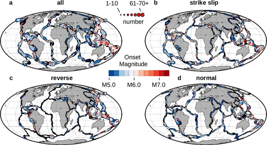
www.nature.com/scientificreports/
risk associated with high magnitude remote triggering. Rather than doing fault-specific analyses, we will develop
a regional analysis to detect the presence of this type of high magnitude triggering. Such an approach could be
used to investigate all tectonic boundaries around the world. Any observations of spatial patterns of remote
triggering would necessarily test our understanding of the underlying processes along tectonic boundaries.
Previous work. General findings on remotely triggered high magnitude e arthquakes8 indicate that trig-
gered events are seen to be preceded within 3 days by large magnitude earthquakes (magnitudes ≥ M6.0) up
to 180° away, and only the largest magnitude events are being triggered. These conclusions were drawn after
the removal of small magnitude events from the input data, along with the removal of data from aftershock
sequences (Methods). Both small-magnitude triggering and aftershock sequences are known triggering pro-
cesses, and their effects were removed from the study. We shall use the approach and findings of that paper as
the basis and starting point for this paper. It is noted that the 3-day time period for triggering gave the strongest
global results, and will be used in this analysis as well.
In the O’Malley et al.8 paper, the observation is made that there are ‘source’ events that initiate the delayed
triggering sequence. Any earthquake of magnitude ≥ M6.0 is a potential source event. Any earthquake of magni-
tude ≥ M5.0 is a potentially triggered event, and it was noted that the USGS catalog used for the study was found
to be complete at this level of detection. The time period that separates the source event from the triggered event
was set at 72 h, although the impact may be longer for the highest magnitude source events.
In that study, aftershocks and foreshocks were removed from the USGS catalog using the windowing tech-
nique applied by Gardner and Knopoff9 (Methods). While there were statistical reasons for applying that method
to decluster the data, the practical result was to avoid biasing the results with aftershock and foreshock data. Also,
when we speak of remote triggering by source events, ‘remote’ is effectively any distance beyond the aftershock
zone of the source event.
Two different numerical experiments were applied in that paper: one that looks forward in time, starting with
potential source events, and one that looks backward in time starting with potentially triggered events. Both
approaches indicated the presence of systematic triggering of medium to high magnitude earthquakes by high
magnitude source events. In this paper we will use the second approach, starting with potentially triggered events.
The variable that was analyzed in that study was the p-value (Methods). Most are familiar with using p-values
to give an estimate of how well data fit a theoretical curve, etc. In this case, however, it is appropriate to think of
it as a basic calculation of probability. What are the odds of getting 5 heads in 7 coin tosses when there’s a 50%
chance of getting heads? What about 15 in 21, or 20 in 28? The p-value keeps dropping even though the ratio of
success remains the same, and is a function of sample size. This is the calculation being applied here.
In this study, the set of potentially triggered events is equivalent to the number of coin tosses. Observa-
tions of the number of ‘heads’ becomes the number of times we find one or more source events preceding the
potentially triggered event within 72 h. And instead of assuming a ‘fair’ coin toss (with a probability of exactly
0.50 of tossing heads or tails) we examine the declustered catalog to find how often potentially triggered events
(M ≥ M5.0) are preceded within three days by one or more potential source events (M ≥ M6.0). Surprisingly, this
ratio is almost exactly equal to 50% (prob = 0.501; Supplemental Information, Section 1). Everything we know
about coin tosses applies here.
In this paper we shall begin with the potentially triggered events and look backwards in time for the source
events. Rather than doing a global analysis of all triggered events, we shall proceed with a local set of events that
fall within a given study area. And the p-value (based on the number of potentially triggered events preceded by
source events, given prob = 0.501) becomes the variable of interest.
Methodology—basic approach. We begin with the declustered, global USGS catalog for all earthquakes
of magnitude ≥ M5.0 from O’Malley et al.8. Those earthquakes are then compared with the results calculated
by the Global Centroid-Moment-Tensor (CMT) Project10,11. When matchups are available, the strike, dip and
rake of the primary focal plane are extracted. The rake is broadly used to classify the type of faulting. A rake of
0° ± 30°, or 180° ± 30° was defined as a strike-slip fault. A rake of − 90° ± 60° is a normal fault (where the hang-
ing wall drops) and a rake of + 90° ± 60° is a reverse (or thrust) fault. Visual examination of a histogram of the
accumulated rakes supports the three distinct populations.
All earthquakes of magnitude ≥ M5.0 that fall within a given project area are extracted from the catalog.
This becomes the set of all potentially triggered earthquakes, and it can be analyzed collectively, or by type of
faulting. The project area used in this paper (Methods) is a bounding box centered on a location of interest and
extending ± 2.85° to the side, normalized for latitude (~ 100,000 k m2 per quadrant).
Each of the potentially triggered earthquakes (M ≥ M5.0) is then examined to see if there exists one or more
source events (M ≥ M6.0) occurring in the previous 72 h from anywhere on the globe. The result is that we have
‘x’ observations of one or more source events for ‘n’ potentially triggered earthquakes. We also know the prob-
ability of seeing one or more source events within 72 h of a potentially triggered event (prob = 0.501). Given
‘x’, ‘n’, and ‘prob’ we can directly apply the binomial theorem to obtain the p-value. In MATLAB12 this is found
using the call for the binomial cumulative distribution function (binocdf). As a note, we will be using the ‘mid’
p-value8, which is the average of the p-values calculated using ‘x’ and ‘x − 1’.
It is possible to apply this method in a manner that indicates how the p-value changes based on magnitude
for a given study area (Methods). For example, if we put in all potentially triggered events, we will have an
estimate of the p-value for all earthquakes with a lower bound of M5.0 and covering all earthquakes up to the
largest observed magnitude. We could then repeat the calculation, but now increasing the lower bound to M5.1.
Then do it again, now starting with a lower bound at M5.2, etc., until it gets up to the maximum magnitude for
the area. What results is a p-value curve as a function of the lower bound magnitude. This p-value curve can be
Scientific Reports | (2022) 12:1138 | https://doi.org/10.1038/s41598-022-05102-4 2
Vol:.(1234567890)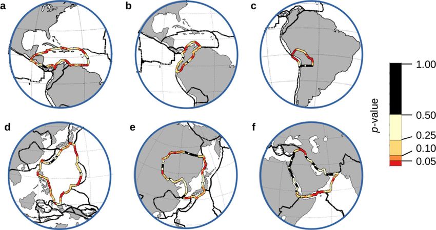
www.nature.com/scientificreports/
Figure 1. Local Detection of Remote Triggering of High Magnitude Earthquakes. The red box (index m aps12)
indicates the area under analysis (± 2.85°, normalized by latitude). The red dot indicates the center of the box.
Black dots represent earthquakes ≥ M5.0 in the region, and red beach balls indicate the focal mechanisms for
oundaries15. Magnitude bins are in tenths of a
thrust events in the study area. Blue dots represent digital plate b
magnitude, ‘M5.0’ only includes data ≥ M5.0 but < M5.1, etc. (a) Earthquakes ≥ M5.0 within the target area are
selected (after removal of aftershocks) and tallied by magnitude (blue bars). Those earthquakes that are preceded
by one or more source events within 3 days are also tallied and overlain in yellow. (b) The ratio of earthquakes
with source events (yellow) to total number of earthquakes (blue) for any given bin is shown in gray bars. The
odds of seeing the combined yellow to blue counts given an average probability of 0.501 are calculated as a
p-value curve (solid line) (see text). The dotted curve plots the − log10 transform of the p-value and locates the
corner associated with the onset magnitude for triggering.
analyzed to determine (1) how susceptible the area is to remote triggering of high magnitude earthquakes, and
(2) what the onset magnitude is for this type of triggering to occur.
Imagine the case of a study area where Eq. (1) is expressed: where high magnitude earthquakes are being
remotely triggered, but where local forces control the lower magnitude earthquakes (no remote triggering for
those magnitudes). The high magnitude earthquakes will have relatively more source events present than the
low magnitude set. The p-value calculated from M5.0 to the maximum magnitude will be higher, approaching
0.5 (or more) since it includes low magnitude events that are non-triggered. As the lower bound is increased, the
number of non-triggered events will decrease (because the lowest magnitudes won’t be counted) and the p-value
will start dropping. At some point the onset magnitude for remote triggering will be reached, and the major-
ity of the non-triggered events will be excluded. With the lower bound set at the onset magnitude, the sample
size will be the largest possible for the triggered events, and the p-value will be a minimum. This minimum in
the p-value locates the onset magnitude for remote triggering, and the p-value for that lower bound indicates
the susceptibility to remote triggering for that study area. Generally speaking, p-values at or above 0.5 indicate
regions of no remote triggering, while regions with p-values below 0.05 will be considered highly susceptible to
such triggering. In practice, there are locations where the p-values get much smaller than 0.05.
Examples of local data analysis. Consider the subduction zone off the coast of Peru, where the Nazca
plate moves under the South American plate as well as the Altiplano microplate. The selected region is very
nearly centered on the junction of these three plates (Fig. 1). The largest earthquake in this region was the mag-
nitude M8.0 Pisco, Peru earthquake of August 15, 200713,14. Significant damage took place at the nearby city of
Pisco.
A total of 140 local earthquakes of magnitude ≥ M5.0 have occurred in the marked region over the past
44 years (excluding aftershocks). Of those 140 earthquakes, the CMT project has 48 focal mechanism solutions
for thrust earthquakes. Given that this is a subduction zone, we will examine these thrust events for our example.
The bounding box used to select earthquakes was ± 2.85°, normalized for latitude (~ 100,000 km2 per quadrant).
The magnitude distribution is shown for these potentially triggered thrust events (Fig. 1a). The number of earth-
quakes in a given bin that were preceded by one or more source events within a three-day period is overlain in
yellow. If only yellow is seen, then all events in that bin were preceded by source events. For magnitude M5.5
and larger, only three earthquakes do not have a preceding source event (22 out of 25 total have source events).
The p-value for this to represent a random drawing is less than 0.0001 (Fig. 1b). The minimum of the resulting
Scientific Reports | (2022) 12:1138 | https://doi.org/10.1038/s41598-022-05102-4 3
Vol.:(0123456789)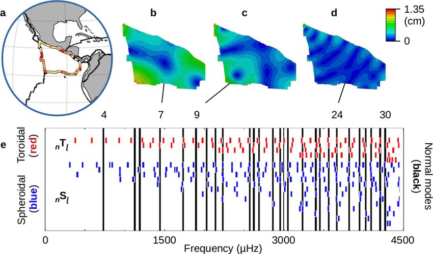
www.nature.com/scientificreports/
Figure 2. Differences in Triggering Based on Type of Faulting. The red boxes (index m aps12) indicate the
area under analysis (± 2.85°, normalized by latitude) for three different sets of earthquakes: (a) reverse, (b)
normal and (c) transform. Focal mechanism are shown for each earthquake set. The blue lines on the map
represent digital plate boundaries15. Magnitude bins for each set are in tenths of a magnitude, ‘M5.0’ only
includes data ≥ M5.0 but < M5.1, etc. Earthquakes ≥ M5.0 within each target area are selected (after removal of
aftershocks) and tallied by magnitude (blue bars). Those earthquakes that are preceded by one or more source
events within 3 days are also tallied and overlain in yellow. The ratio of earthquakes with source events (yellow)
to total number of earthquakes (blue) for any given bin is shown in gray bars. The odds of seeing the combined
yellow to blue counts given an average probability of 0.501 are calculated as a p-value curve (solid line) (see
text). The dotted curve plots the -log10 transform of the p-value and locates the corner associated with the onset
magnitude for triggering. Reverse and transform faulting shows strong triggering, while normal faults are not
being triggered in this locale.
p-value curve is used to indicate the onset for remote triggering of high magnitude events. The onset magnitude
is most easily seen by looking for the corner in the p-value curve when plotted as − log10(p-value) (dotted line).
For the boxed region off the coast of Peru, the triggering zone begins at M5.5 and has an associated p-value
of < 0.0001 for all events from M5.5 up to the highest magnitude earthquake of the region. A p-value of exactly
0.0001 indicates that there is one chance in 10,000 that the observed pattern is simply a random expression of
the general probability. This region has been highly susceptible to remote triggering of high magnitude thrust
earthquakes over the past 40 + years. See Supplemental Information, Section 3 for the global distribution of the
source events associated with these events.
For the next example we will consider a region identified as an oceanic convergence zone (Fig. 2). In this case
we will examine the results for all three major types of faulting. As in the case for the subduction zone, earth-
quakes with reverse (thrust) faults (Fig. 2a) strongly indicate the presence of triggering, with 19 of 23 earthquakes
at or above M6.0 having source events (p-value = 0.0008). However, earthquakes with normal faults do not exhibit
any triggering at all for high magnitude events (Fig. 2b). The p-values for normal faulting in this zone of overall
convergence never gets below 0.60. This implies that normal faulting is entirely controlled by local forces in this
area. Transform faulting for the same region (Fig. 2c) shows the presence of triggering similar to reverse fault-
ing, with 14 out of 17 earthquakes having source events at or above M5.9 (p-value = 0.0039). See Supplemental
Information, Section 3 for the distribution of source events associated with Fig. 2a, c.
Results for the plate boundaries
The above approach makes it possible to map the plate boundaries for their susceptibility to remote triggering of
high magnitude earthquakes. The method can be applied systematically across the globe given digital locations
that delineate the plates15. This can be done for all earthquakes combined, or for subsets based on focal mecha-
nism (normal, reverse, or strike-slip earthquakes). The results show an extensive global presence of this type of
delayed triggering (Fig. 3), whether analyzed collectively, or individually based on focal mechanism. Suscepti-
bility to triggering is more pervasive for strike-slip than it is for for normal or thrust faulting. The p-values for
strike-slip earthquakes are also more skewed to lower values than the other two types of faulting. The collective
results (Fig. 3a) can be examined to test the global susceptibility to high magnitude triggering, regardless of focal
Scientific Reports | (2022) 12:1138 | https://doi.org/10.1038/s41598-022-05102-4 4
Vol:.(1234567890)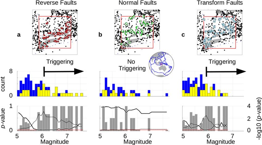
www.nature.com/scientificreports/
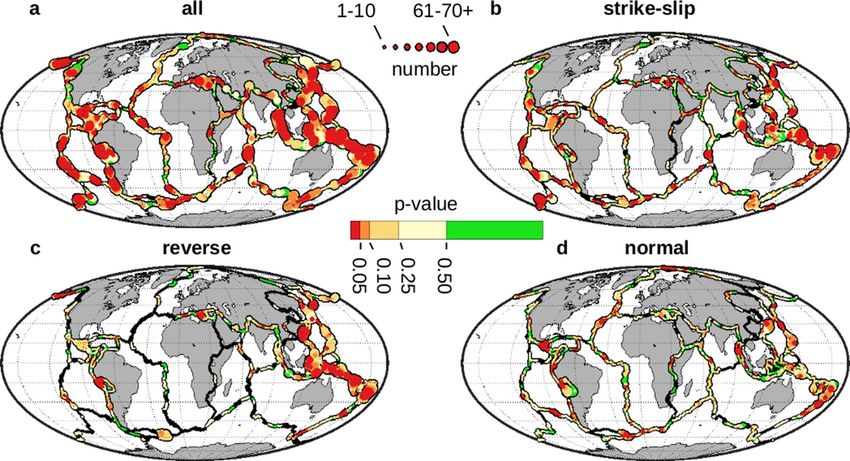
Figure 3. Plate boundaries susceptible to remote triggering of high magnitude earthquakes. Each location
of the digital plate boundaries15 is locally tested for remote triggering of high magnitude earthquakes. The
p-value for the triggering zone becomes the variable of interest and represents the susceptibility to this type of
remote triggering. Green represents those areas with no susceptibility (p-values ≥ 0.50) while the highest level
of susceptibility (red) is for p-values < 0.05. Black indicates no data. Line widths are scaled to the number of
potentially triggered earthquakes at each location. (a) This is the global map12 that results when all earthquakes
are combined and shows susceptibility to earthquakes taken collectively. (b) These are the results when only
considering potentially triggered events with strike-slip faulting. They show a global prevalence to triggering
of strike-slip faulting and represent many of the features seen in (a). (c) Susceptibility to triggering for reverse
(thrust) faulting. (d) These are the patterns when only considering normal faulting for the potentially triggered
events.
mechanism. Plate boundary locations that do not exhibit this behavior (p-values ≥ 0.50; 14% of the locations)
are shown in green, while 86% of the plate boundaries exhibit susceptibility to varying degrees. Those locations
that are the most susceptible are shown in red, with p-values < 0.05 (19%).
The associated onset magnitudes for remote triggering of high magnitude earthquakes are also available
(Fig. 4). These results can also be obtained collectively, or based on focal mechanism. For the collective case, a
majority of the plate boundaries (65%) are seen to have onset magnitudes that are below M6.0 (shown in blue).
The onset magnitude for remote triggering is potentially equivalent to the upper corner magnitude ( MC) of
the modified Gutenberg–Richter formula (Eq. 1). MC is used in probabilistic estimates for regional s eismicity7,16,17
and a variable proxy via the onset magnitude for remote triggering could be useful. The onset magnitude defined
here is a new metric based on a regional analysis, and it delivers results based on data spanning 40 + years. For
comparison, Boettcher and M cGuire4 give M
C magnitude values for mid-ocean ridge transform faults of Gofar
(segments G1, G2 and G3), and Discovery (segments D1 and D2). These five combined Gofar and Discovery
segments in the East Pacific Rise are located within a single box in this study. The result found here was an onset
magnitude of M6.1 for the strike-slip subset, which is comparable to the reported MC values of M6.1, M5.8, M6.2,
M5.6 and M6.0 for the individual segments. However, Boettcher and M cGuire4 also report an MC value of M6.4
for the Blanco Ridge, but here the best example that isolates the transform faults of the Blanco Ridge yields an
onset magnitude that is much lower (M5.1).
Generalized MC estimates are available for different tectonic settings, combining global statistics and model
considerations18. They show that the M C value for subduction zones is the largest of all possible plate boundaries.
They also show that convergent boundaries have larger MC values than divergent boundaries, and transform/
strike-slip boundaries fall in between the two. However, their estimates of M C are consistently greater than the
onset magnitudes obtained here, and we will return to this in the Discussion section. For example, the high-
est onset magnitudes obtained in this study are M8.4, found along a segment where the Pacific Plate subducts
under the Okhotsk Plate at 40° N latitude just east of Japan. Bird and Kagan18 report M9.58 (+ 0.48/-0.46) as
representative of global subduction zones. Moreover, here the onset magnitude appears to be a function of the
susceptibility to remote triggering: the higher the susceptibility the lower the onset magnitude (Fig. 5). The data
were separated by plate boundary type and focal mechanism, and the onset magnitudes were averaged for three
p-value bins (0.0–0.1, 0.1–0.2, and 0.2–0.3). Standard errors are shown to indicate the possible range in the
calculated averages, and best fit lines were projected. The trace for the subduction zone is clearly greater than
Scientific Reports | (2022) 12:1138 | https://doi.org/10.1038/s41598-022-05102-4 5
Vol.:(0123456789)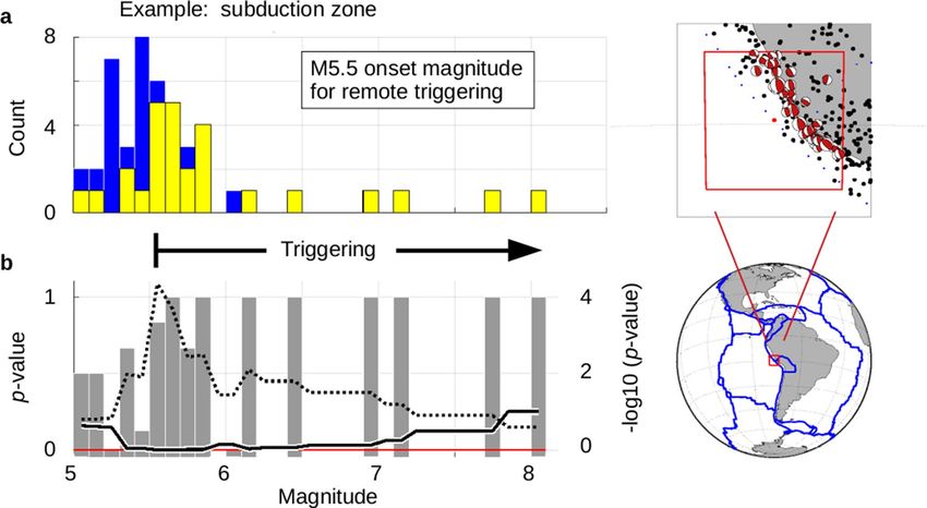
www.nature.com/scientificreports/
Figure 4. Onset magnitudes for remote triggering of high magnitude earthquakes. Each location of the
digital plate boundaries15 is locally tested for remote triggering of high magnitude earthquakes. Global m aps12
of the onset magnitude for this type of triggering are shown for different collections of potentially triggered
earthquakes: (a) all combined, (b) strike-slip only, (c) reverse only, and (d) normal only. The onset magnitudes
shown here are associated with the p-values shown in Fig. 3. Line widths are scaled to the number of potentially
triggered earthquakes at each location. No onset magnitudes are shown for those locations that do not express
this type of triggering (shown in black).
Figure 5. Onset magnitude as a function of remote triggering p-value. P-values were separated by the seven
different boundary types and associated focal, then the onset magnitudes were binned as a function of p-value:
0.0–0.1, 0.1–0.2 and 0.2–0.3. The average for each bin is shown; error bars indicate the standard error to show
how much variation in the average is possible. The results for subduction zones (black dashed line) gives the
highest onset magnitude for all boundary types, and is shown on both plots for reference. (a) Results for oceanic
boundary types (convergent, transverse and divergent). (b) Results for continental boundary types (convergent,
strike-slip and divergent). Mc v alues18 are shown to illustrate the range found in their study.
Scientific Reports | (2022) 12:1138 | https://doi.org/10.1038/s41598-022-05102-4 6
Vol:.(1234567890)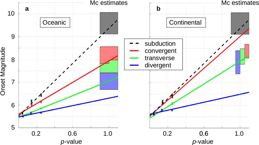
www.nature.com/scientificreports/
Figure 6. Spatial patterns of susceptibility to remote triggering around individual plates. Consistent patterns
lates12, while varying from
of highs and lows in susceptibility to triggering are seen surrounding individual p
plate to plate (data extracted from Fig. 3a). Constant p-value line widths were used to illustrate the patterns. (a)
Caribbean plate. (b) North Andes plate. (c) Altiplano plate. (d) Philippine Sea plate. (e) Amur plate. (f) Arabia
plate.
all other boundary types, and the order of convergent > transform > divergent is seen for both oceanic (Fig. 5a)
and continental (Fig. 5b) plates. The colored boxes on the right of the plots show a range of M
C values resulting
from Bird and Kagan’s18 work.
Given the global extraction of p-values and onset magnitudes based on focal mechanism, we were able to test
the uniqueness of our observed results against synthetic (time-randomized) earthquake catalogs. We compared
the value of the projected onset magnitude shown in Fig. 5 (at p-value = 1.0) with values obtained from synthetic
catalogs for the seven different tectonic regimes (Supplemental Information, Section 2, Fig. 5). The observed
data shown in Fig. 5 resulted in extreme values when compared with 64 of the 70 random results. The p-value
associated with that test of randomness is on the order of 1e-14.
Patterns of susceptibility and normal modes of the Cocos plate. Local patterns of highs and lows
in the susceptibility to remote triggering are present throughout the map of the combined earthquakes (Fig. 3a),
from the tight, alternating pattern of the Caribbean plate to the broader spacing seen at the triple junction in the
north Atlantic. Closer inspection shows that the local spacing appears to vary from plate to plate (Fig. 6). While
similarities may be found, such as the simple two-high pattern surrounding the Altiplano plate (6c) and the Ara-
bia plate (6f.), the lengths of the quiescent zones are much different. Similar comparisons can be made between
Fig. 6a, d, as well as Fig. 6b, e. These patterns cross all plate boundary types. Spatial patterns in susceptibility
which surround individual plates seem to imply some form of physical mechanism at play. If so, this unknown
mechanism is somehow impacting the local susceptibility to remote triggering by modifying the boundary con-
ditions, which includes lowering the onset magnitudes.
A potential mechanism that we will consider is thin-plate resonance. We check for two aspects to be present to
verify if the normal modes of the plate should be considered as a possible factor impacting the boundary condi-
tions along the edges of the plate. First, are there alignments of increased susceptibility with observed patterns in
the various normal modes for the plate? If so, then the next becomes: what is driving the resonance? The answer
to this will be found in the natural frequencies of the calculated normal modes. If there are global processes
available with similar frequencies to drive the normal modes, then we have the potential for a mechanism to be
involved with this type of high-magnitude delayed triggering.
Our initial test is on the Cocos plate (Fig. 7a), which is somewhat triangular in shape and composed only of
oceanic crust. The spacing between its susceptibility highs is about twice that of the Caribbean plate (Fig. 6a)
although the areas of the two plates are quite similar. We constructed a finite element model (FEM) of the Cocos
plate for input into Abaqus 6.14–119. Plate boundary l ocations15 were used to define the edges of the Cocos plate,
and a thickness of ~ 11 km (0.1° arc distance) was uniformly applied. For this initial model we did not add a slab
to represent the subducting section diving to the northeast20. Density, Young’s modulus and Poisson’s ratio for
oceanic crust were obtained from an FEM off the coast of P eru21. The bottom of the plate was pinned to allow
motion only in the ij-plane (horizontally) and represents plate movement along the top of the lower lithosphere.
Scientific Reports | (2022) 12:1138 | https://doi.org/10.1038/s41598-022-05102-4 7
Vol.:(0123456789)
www.nature.com/scientificreports/
Figure 7. Normal Modes of the Cocos plate. (a) Data for the susceptibility to remote triggering extracted from
Fig. 3a12. The most susceptible location is on the western face, with a p-value of 0.004. Other secondary highs are
visible on the eastern diagonal edge and to the south. (b–d) Examples of normal modes are shown for the Cocos
plate19. Plots are set to the same displacement scale (color bar shown). Blue represents nodal lines at the extreme.
All three examples have nodal lines matching up with the main susceptibility high on the western edge along
with the eastern diagonal edge. Alignment with other secondary highs is present as well. (b) Normal mode 7. (c)
Normal mode 9. (d) Normal mode 24. (e) Natural frequencies are shown for normal modes 4 to 30 (black lines).
Overlain are frequencies for toroidal (red) and spheroidal (blue) free o scillations22. The toroidal and spheroidal
frequencies are organized by overtones. The top row of each represents the fundamental frequencies (0Tℓ and
0Sℓ), the next row represents the 1st overtones (1Tℓ and 1Sℓ), etc. Free oscillations of the earth are available to
drive a number of the normal modes of the Cocos plate.
Initial results indicate examples of displacement magnitudes for normal modes for the Cocos plate with
features that align with the primary susceptibility location on the western boundary, as well as other second-
ary highs (Fig. 7b–d). Please note that the amplitude of the normal mode displacement is not absolute, as each
mode will be scaled in specific application. The frequency range of modes 4 to 30 covers 730.7 to 4270.8 μHz,
or periods ranging from 22.8 to 3.9 min (Fig. 7e). These values are within the frequency range of toroidal and
spheroidal free oscillations of the e arth22 (Fig. 7e). Free oscillations (planetary standing waves) are regularly
produced following large magnitude earthquakes. The source events (M ≥ M6.0) that precede the potentially
triggered events (M ≥ M5.0) are large enough to generate free oscillations and can therefore stimulate specific
normal modes of the plate.
We propose that specific normal modes can induce triggering (a failure along the fault plane) dependent
on the associated stress. The units of stress are force per unit area, and stress is a tensor (not a vector). Positive
stress normal to a plane represents bidirectional expansion, while negative stress represents compression. Here
we consider what happens if we have a one-sided change in the stress field near a fault plane, but not on the other
(for example, a change in the stress in the Cocos Plate but not the Pacific Plate). If we have a unit cell on one
side a fault plane, then positive stress normal to the fault plane will expand into the fault plane, while negative
stress represents a contraction away from the fault plane. If a one-sided contraction occurs in the stress normal
to the fault plane, then the force binding the fault plane together will be reduced. Reduce the force sufficiently
and a fault rupture will follow.
We can do an initial test for the presence of this triggering using the data for the Cocos plate. The susceptibility
high that is seen along the western edge of the Cocos Plate is due to transverse faulting. A simplified version of the
transverse p-values for the Cocos Plate (Fig. 8a) shows all p-values < 0.10 as black circles and all p-values between
0.10 and 0.50 are cyan. We also have a representation of the perimeter stress values for mode 24 (Fig. 8b). Here
we have compared the sign of the S11 (north–south) stress with the sign of the S22 (east–west) stress. If both are
positive, we have pure horizontal expansion (red), while if both are negative we have pure horizontal compression
(black). A scatter diagram of the p-values less than 0.1 versus the S22 stress (Fig. 8c) shows the majority of the
susceptible locations also have negative (contracting) horizontal stress present. While some of the dots overlay
Scientific Reports | (2022) 12:1138 | https://doi.org/10.1038/s41598-022-05102-4 8
Vol:.(1234567890)www.nature.com/scientificreports/
Figure 8. Comparison of Susceptibility to Triggering and Horizontal Stress. (a) Susceptibility of transform
faults to remote triggering is shown in simplified form, with black circles for p-values < 0.1, and cyan dots for
0.1 < p-value < 0.5. The location of the highest susceptibility is on the western edge of the Cocos plate. (b) A
representation of the perimeter stress due to normal mode 24 is shown. If the horizontal components (S11
and S22) are both positive, a red dot is shown; if the horizontal components are both negative, a black circle is
shown. Small blue dots show those locations where S11 and S22 have opposite signs. (c) A scatter diagram of
the highly susceptible p-values in (a) versus the E–W stress component (S22) of mode 24. A strong matching of
negative (compressive) stress with remote triggering of transverse faulting is present.
each other, a tabulation shows that 22 of the 30 p-values < 0.10 are associated with negative horizontal stress. A
matchup rate of 22 of 30 yields a p-value of 0.0053. Comparison of these results with ten synthetic catalogs for
strike-slip events (Supplemental Information, Section 2, Fig. 8c) shows that randomized data give p-value results
that range from 0.994 to 0.004, while the observed data has a higher matchup rate (smaller p-value) than 9 of
10 random catalogs. The results from the data shown in Fig. 8c are significant when compared with synthetic
catalogs. The pattern in the observed data supports the idea that a temporary increase in negative horizontal
stress may be involved in the triggering mechanism, while comparison with synthetic catalogs confirms this is
not a random result.
Discussion
The method developed here to detect the local expression of remotely triggered high magnitude earthquakes
(Figs. 1, 2) is essentially a local test based on the retrospective analysis of Experiment 2 of the previous study that
presented high magnitude, remote triggering by global source events8. The resulting p-values are interpreted
globally as a metric that indicates local susceptibility to remote triggering (Fig. 3). The primary conclusion of
the previous paper asserting the existence of systematic triggering from anywhere beyond the aftershock zone
(up to 180° away) is consistent with the results here (Supplemental Information, Section 3).
Testing for the local presence of remote triggering also yielded estimates of the globally varying onset mag-
nitude for remote triggering (Fig. 4). Above this onset magnitude only relatively small perturbations are needed
to trigger earthquakes; below this magnitude stronger forces are required. A ‘reality check’ on the results was
to compare the onset magnitudes with observations of M C, both local studies and global analyses. While the
onset magnitude was consistent with some results of local seismic studies, they in general were lower than the
calculated values for the seven types of plate boundaries. We later suspected that the triggering magnitude was
being lowered by a physical process that was modifying the boundary conditions along the fault planes. Given
the observation of negative horizontal stress matching up with the low p-value results of transverse faults (Fig. 8),
a temporary reduction in the normal forces along the fault plane could be involved, effectively reducing Mc
to the observed onset magnitudes. It is noted that a linear relationship appears to be in the data between the
p-value of triggering and the onset magnitude (Fig. 5) and that projecting the onset magnitudes to p-values of
1.0 gives approximate match-ups with Mc estimates. The onset magnitude progression of convergent > trans-
verse > divergent boundaries (with subduction being the greatest) was also consistent with the progression seen
in global analysis of M C.
Patterns of p-values around individual plates appeared to be quite distinct (Fig. 6), which led to the specula-
tion that an external process could be modifying the boundary conditions along the edges of the plates. Such a
process would also be responsible for lowering the values of MC to the observed onset magnitudes. We explored
one such possibility with an FEM model analyzing thin-plate resonance of the Cocos plate. More significant
than the specific patterns present in the various normal modes of the Cocos plate were their natural frequencies
(Fig. 7). In the case of the Cocos plate, the natural frequencies can be driven by a variety of frequencies associ-
ated with global free oscillations (Fig. 7e).
Given the possibility of normal modes of the Cocos plate being driven by specific free oscillations following
source events with magnitudes ≥ M6.0, the stress tensors for normal mode 24 were examined for overall hori-
zontal expansion or compression along the perimeter of the plate. Comparison with p-values for transform faults
(0.0–0.10) showed overall association of compressive stress regimes associated with susceptibility to triggering.
Scientific Reports | (2022) 12:1138 | https://doi.org/10.1038/s41598-022-05102-4 9
Vol.:(0123456789)www.nature.com/scientificreports/
We suggest that the original source events (M ≥ M6.0) drive the normal mode responses of the individual plates
via free oscillations, creating a mechanism for delayed triggering. As those normal modes are established, they
eventually generate sufficient negative stress normal to the local fault planes, and triggered events (M ≥ M5.0)
ensue.
Conclusions
A method for analyzing a local region’s susceptibility to remote triggering is presented. While it was applied here
in a uniform fashion across all plate boundaries, it can also be ‘tuned’ to a specific region. The size of the target
area being tested may be smaller, change shape, or be rotated as the specific context dictates. Also obtained by
this method is an empirical estimate of the onset magnitude for triggering to occur. Researchers may find this
to be an appropriate proxy for a variable MC in their local earthquake hazard analyses.
A three-day time period between source event and triggered event is present in the calculations, but the
mechanisms implied by this delay are not specified. An intriguing possibility is that resonance of entire tectonic
plates is involved, resonance driven by free oscillations created by the high magnitude source events themselves.
As the individual modes are established in the hours that follow, the deviatoric stress associated with those modes
builds upon the existing fault planes. Sufficient one-sided negative stress normal to the fault planes could release
the triggered events.
Methods
Global data. Earthquake data were obtained from the United States Geological Survey (USGS) archives23 for
all earthquakes with magnitudes ≥ M5.0. The time period covered goes from the start of 1973 through the end of
2016. A minimum threshold of M5.0 for data going back to 1979 was determined to be globally detectable in a
previous study24. This is confirmed in the current set by examining the magnitude-frequency distribution of the
data. No roll off or corner frequency is observed in the data used for this study as the magnitudes drop to M5.0.
Additionally, predicted b-value counts are within 0% to -6% of the observed totals for magnitudes below M5.5.
With no observable drop-off in the earthquake counts at the lowest magnitudes used in this study, we conclude
that the global catalog is complete when using a threshold of M5.0.
These data were then compared with the results calculated by the Global Centroid-Moment-Tensor (CMT)
Project10,11. When match-ups were available, the rake of the primary focal plane was used to classify the type of
faulting. A rake of 0° ± 30°, or 180° ± 30° was defined as a strike-slip fault. A rake of − 90° ± 60° is a normal fault
(where the hanging wall drops) and a rake of + 90° ± 60° is a reverse (or thrust) fault.
Filtering out aftershocks. Care is taken to remove known clustering processes from this analysis using a
standard declustering technique. The number of aftershocks follow distribution patterns based on the magnitude
of the main event, such as the ‘epidemic type’ m odel25. Our concern here is to decluster the data over time and
remove the effects of this known triggering process.
The declustering method selected was the windowing technique applied by Gardner and K nopoff9. While this
method is easy to implement, importantly the temporal distribution of the earthquakes in the declustered catalog
follows a Poisson distribution9,26. Using this method, an earthquake has both a spatial and a temporal extent
which are functions of magnitude. The equations used are given in Eq. (1) of van Stiphout et al.26. Specifically,
the distance window (in kilometers) is estimated by 100.1238M+0.983. The time window (in days) has one curve for
M6.5 and larger (100.032M+2.7389) and another for smaller magnitudes (100.5409M-0.547). The temporal extent can be
quite significant, as data from large magnitude events extend hundreds of days. For example, the time window
for M5.0 covers 144 days, M6.0 goes 499 days, M7.0 is at 918 days, and M8.0 extends to 988 days. Similarly,
the distance window for M5.0 covers 40 km, M6.0 is at 53 km, M7.0 spans 71 km, and M8.0 extends to 94 km.
Data that fall in the combined spatial and temporal windows, either before or after a main event, are flagged as
aftershocks or foreshocks and removed from the subsequent analysis.
Data selection for a project area. Given a latitude and longitude (lat0 and lon0) for a location of inter-
est, the global data (filtered for aftershocks) are searched to locate all earthquakes within a box defined by a
minimum and maximum latitude and longitude. The bounding box in this study is defined by lat0 + /− dlat and
lon0 +/− dlon, where dlat is set at 2.85° latitude and dlon is set at 2.85/sin(90-lat0) degrees longitude.
Once a bounding box is defined, the global data set (with aftershocks removed) is searched for any earth-
quakes with magnitudes M5.0 or larger within the project area. This is the set of potentially triggered events.
The global data set is then searched again for any earthquakes of magnitude M6.0 or larger from anywhere on
the globe that took place within 72 h of the potentially triggered events. These large, global earthquakes are the
source events. We now have ‘n’ potentially triggered events, and ‘x’ of those are preceded by one or more source
events within 72 h. An analysis of the global set used in this study shows that the probability of observing one or
more source events within 72 h of a potentially triggered event has a probability of 0.501. This value is applied
to all regions.
Calculation of p‑values. The general binomial distribution is of the form
(n−x)
f(x) = [n!/(n − x)!] ∗ px ∗ 1 − p (2)
The first part (with factorials) is generally read “n choose x” where ‘x’ is the number of successes out of ‘n’
trials, and the probability ‘p’ gives the probability of a success.
Scientific Reports | (2022) 12:1138 | https://doi.org/10.1038/s41598-022-05102-4 10
Vol:.(1234567890)www.nature.com/scientificreports/
Each project area supplies ‘n’ earthquake counts of potentially triggered events. The number of triggered
events with observed source events in the preceding 72 h plays the role of ‘x’ in the binomial distribution. The
random probability of having such a ‘success’ for the global set used in this study was found to be 0.501.
What is now needed is a cumulative probability function for the binomial distribution which will give the
27, this is given by the function ‘pbinom’. If cpf = pbinum(count,
total probability of getting up to ‘x’ successes. In R
size, prob), then the p-value is given by 1 − cpf. The p-value thus gives the probability that the random probability
0.501 could deliver a count of ‘x’ or more.
The last detail is that we calculate the mid p-value28 using [count − 0.5] instead of the traditional p-value, to
avoid the known bias appearing in the binomial calculation based on discrete quantity that take only integer
numbers (such as earthquake counts).
Algorithm for analysis. We wish to evaluate the p-values as a function of magnitude for a given project
area. The p-value will then be associated with earthquakes within a magnitude range that runs from a lower
bound to an upper bound. The upper bound is set at the maximum magnitude event within the project area.
The lower bound is iteratively adjusted to cover the range from M5.0 to the upper bound magnitude. The results
yield a p-value curve which is a function of the lower bound magnitude, running from M5.0 to the maximum
observed earthquake in the area.
Given the p-value curve running from M5.0 to the maximum magnitude event, it is now searched for the
magnitude with the minimum p-value. In general, this is visually easy to locate if one plots a -log10 transform
of the p-value curve. The onset magnitude for triggering becomes the magnitude with the minimum p-value for
this project area. The minimum p-value indicates the susceptibility to remote triggering within the bounding box.
Onset magnitude detail. The simplest version of this algorithm locates the magnitude associated with
the actual minimum p-value and assigns that magnitude as the onset magnitude for remote triggering. For
p-values smaller than 0.05, however, it was of interest to see how low the magnitude would go while still allow-
ing the overall p-value to still be less than 0.05 (highly susceptible to triggering). The onset magnitude in this
case indicates an overall p-value zone that is less than 0.05. An additional adjustment for this particular situation
is to make sure the ratio of source events to total events for the onset magnitude bin is greater than the general
probability of 0.501. If it isn’t, the onset magnitude is increased by one bin and tested again (each bin spans one
tenth of a magnitude). When done in this fashion, the algorithm picks onset magnitudes consistent with those
found by visual inspection of the data.
Received: 14 October 2020; Accepted: 5 January 2022
References
1. Scholz, C. H. Large earthquake triggering, clustering, and the synchronization of faults. Bull. Seismol. Soc. Am. 100, 901–909
(2010).
2. Gomberg, J., Bodin, P., Larson, K. & Dragert, H. Earthquake nucleation by transient deformations caused by the M = 7.9 Denali,
Alaska, earthquake. Nature 427, 621–624 (2004).
3. McGuire, J. J. Seismic cycles and earthquake predictability on East Pacific Rise transform faults. Bull. Seismol. Soc. Am. 98,
1067–1084 (2008).
4. Boettcher, M. S. & McGuire, J. J. Scaling relations for seismic cycles on mid-ocean ridge transform faults. Geophys. Res. Lett. 36,
L21301 (2009).
5. Perfettini, H. & Avouac, J. P. The seismic cycle in the area of the 2011 Mw9.0 Tohoku-Oki earthquake. J. Geophys. Res. Solid Earth
119, 4469–4515 (2014).
6. Goldfinger, C. et al. Turbidite event history—Methods and implications for Holocene paleoseismicity of the Cascadia subduction
zone. U.S. Geol. Surv. Profess. Pap. 1661-F, 1–184 (2012).
7. Kagan, Y. Y. & Jackson, D. D. Probabilistic forecasting of earthquakes. Geophys. J. Int. 143, 438–453 (2000).
8. O’Malley, R. T., Mondal, D., Goldfinger, C. & Behrenfeld, M. Evidence of systematic triggering at teleseismic distances following
large earthquakes. Sci. Rep. 8, 11611. https://doi.org/10.1038/s41598-018-30019-2 (2018).
9. Gardner, J. K. & Knopoff, L. Is the sequence of earthquakes in Southern California, with aftershocks removed, Poissonian?. Bull.
Seismol. Soc. Am. 64, 1363–1367 (1974).
10. Dziewonski, A. M., Chou, T.-A. & Woodhouse, J. H. Determination of earthquake source parameters from waveform data for
studies of global and regional seismicity. J. Geophys. Res. 86, 2825–2852 (1981).
11. Ekström, G., Nettles, M. & Dziewonski, A. M. The global CMT project 2004–2010: Centroid-moment tensors for 13,017 earth-
quakes. Phys. Earth Planet. Inter. 200–201, 1–9 (2012).
12. MATLAB Release 2020b, The MathWorks, Inc, Natick, MA, USA. https://www.mathworks.com.
13. Tavera, H. & Bernal, I. The Pisco (Peru) earthquake of 15 August 2007. Seismol. Res. Lett. 79, 510–515 (2008).
14. Sladen, A. et al. Source model of the 2007 Mw 8.0 Pisco, Peru earthquake: Implications for seismogenic behavior of subduction
megathrusts. J. Geophys. Res. Solid Earth 115, B02405-B2411 (2010).
15. Bird, P. An updated digital model of plate boundaries. Geochem. Geophys. Geosyst. 4, 1027. https://doi.org/10.1029/2001GC0002
52 (2003).
16. Field, E. H. Overview of the working group for the development of regional earthquake likelihood models (RELM). Seismol. Res.
Lett. 78, 7–16 (2007).
17. Talebi, M., Zare, M., Peresan, A. & Ansari, A. Long-term probabilistic forecast for M ≥ 5.0 earthquakes in Iran. Pure Appl. Geophys.
17, 1561–1580 (2017).
18. Bird, P. & Kagan, Y. Y. Plate-tectonic analysis of shallow seismicity: Apparent boundary width, beta, corner magnitude, coupled
lithosphere thickness, and coupling in seven tectonic settings. Bull. Seismol. Soc. Am. 94, 2380–2399 (2004).
19. Dassault Systèmes SIMULIA (2017). http://www.3ds.com.
Scientific Reports | (2022) 12:1138 | https://doi.org/10.1038/s41598-022-05102-4 11
Vol.:(0123456789)www.nature.com/scientificreports/
20. Kim, Y., Clayton, R. W. & Jackson, J. M. Geometry and seismic properties of the subducting Cocos plate in central Mexico. J.
Geophys. Res. Solid Earth 115, B06310 (2010).
21. Salomon, C. Finite element modelling of the geodynamic processes of the Central Andes subduction zone: A reference model.
Geod. Geodyn. 9, 246–251 (2018).
22. Masters, T. G. & Widmer, R. Free oscillations: frequencies and attenuations. In Global Earth Physics: A Handbook of Physical
Constants 104–125 (ed. Ahrens, T. J.) (AGU, 1995).
23. Data obtained from the United States Geological Survey’s Earthquake Hazards Program at http://e arthq uake.u
sgs.g ov/e arthq
uakes/
(2017).
24. Parsons, T. & Geist, E. L. The 2010–2014.3 global earthquake rate increase. Geophys. Res. Lett. 41, 4479–4485 (2014).
25. Ogata, Y. Statistical model for standard seismicity and detection of anomalies by residual analysis. Tectonophysics 169, 159–174
(1989).
26. van Stiphout, T., Zhuang, J. & Marsan, D. Seismicity declustering. Community Online Resource for Statistical Seismicity Analysis
10, 1–25 (2012).
27. Team, R. C. R: A language and environment for statistical computing. 3–26 (R Foundation for Statistical Computing, Vienna, Austria,
2014).
28. Lancaster, H. O. Significance tests in discrete distributions. J. Am. Stat. Assoc. 56, 223–234 (1961).
Acknowledgements
Earthquake archives were initially obtained from the United States Geological Survey’s Earthquake Hazards
Program at http://earthquake.usgs.gov/e arthquakes/ (2017). The author would like to thank MJB for his support
and encouragement throughout this analysis.
Author contributions
R.T.O. ran all numerical experiments on earthquake data, A.C. performed all FEM modeling, and Y.Z. supervised
the FEM modeling.
Competing interests
The authors declare no competing interests.
Additional information
Supplementary Information The online version contains supplementary material available at https://doi.org/
10.1038/s41598-022-05102-4.
Correspondence and requests for materials should be addressed to R.T.O.
Reprints and permissions information is available at www.nature.com/reprints.
Publisher’s note Springer Nature remains neutral with regard to jurisdictional claims in published maps and
institutional affiliations.
Open Access This article is licensed under a Creative Commons Attribution 4.0 International
License, which permits use, sharing, adaptation, distribution and reproduction in any medium or
format, as long as you give appropriate credit to the original author(s) and the source, provide a link to the
Creative Commons licence, and indicate if changes were made. The images or other third party material in this
article are included in the article’s Creative Commons licence, unless indicated otherwise in a credit line to the
material. If material is not included in the article’s Creative Commons licence and your intended use is not
permitted by statutory regulation or exceeds the permitted use, you will need to obtain permission directly from
the copyright holder. To view a copy of this licence, visit http://creativecommons.org/licenses/by/4.0/.
© The Author(s) 2022
Scientific Reports | (2022) 12:1138 | https://doi.org/10.1038/s41598-022-05102-4 12
Vol:.(1234567890)You can also read