Review and recommendations for univariate statistical analysis of spherical equivalent prediction error for IOL power calculations
←
→
Page content transcription
If your browser does not render page correctly, please read the page content below
65

                                                                         ARTICLE

                 Review and recommendations for
             univariate statistical analysis of spherical
                equivalent prediction error for IOL
                         power calculations
           Jack T. Holladay, MD, MSEE, Rand R. Wilcox, PhD, Douglas D. Koch, MD, Li Wang, MD, PhD

   Purpose: To provide a reference for study design comparing                       PE distributions were not normal, but symmetric and lepto-
   intraocular lens (IOL) power calculation formulas, to show that the              kurtotic (heavy tailed) and had higher peaks than a normal
   standard deviation (SD) of the prediction error (PE) is the single               distribution. The absolute distributions were asymmetric and
   most accurate measure of outcomes, and to provide the most                       skewed to the right. The heteroscedastic method was much
   recent statistical methods to determine P values for type 1 errors.              better at controlling the probability of a type I error than older
                                                                                    methods.
   Setting: Baylor College of Medicine, Houston, Texas, and Uni-
   versity of Southern California, Los Angeles, California, USA.
                                                                                    Conclusions: (1) The criteria for patient and data inclusion were
                                                                                    outlined; (2) the appropriate sample size was recommended; (3) the
   Design: Retrospective consecutive case series.                                   requirement that the formulas be optimized to bring the mean error
                                                                                    to zero was reinforced; (4) why the SD is the single best parameter
   Methods: Two datasets comprised of 5200 and 13 301 single                        to characterize the performance of an IOL power calculation
   eyes were used. The SDs of the PEs for 11 IOL power calculation                  formula was demonstrated; and (5) and using the heteroscedastic
   formulas were calculated for each dataset. The probability density               statistical method was the preferred method of analysis was
   functions of signed and absolute PE were determined.                             shown.

   Results: None of the probability distributions for any formula                   J Cataract Refract Surg 2021; 47:65–77 Copyright © 2020 Published by
   in either dataset was normal (Gaussian). All the original signed                 Wolters Kluwer on behalf of ASCRS and ESCRS

                                                                                    with 3 or more the Friedman test.2–5 They also pointed out

A
         PubMed search of the past 5 years revealed 239
         articles published on intraocular lens (IOL) power                         that, if the P value is not statistically significant, post hoc
         calculation formulas. The sample sizes ranged from 1                       analysis can be performed to find out which group or groups
to 18 001 cases, and outcomes of mean prediction error (PE),                        are responsible for the null hypothesis being rejected, which
mean absolute PE, median PE, associated SDs, and mean                               might be used to correct for the multiple comparisons made
absolute deviations (MADs) were reported. There was no                              as recommended by Benavoli et al.6 We disagree with the
consistency in the reporting or the statistical methods used to                     comments by Aristodemou et al. and the response offered by
compare formulas, techniques, or devices, although most                             Hoffer et al and will recommend current statistical tech-
converted to absolute values for the statistical analysis.                          niques that overcome errors in the P value of the not normal,
   In their article in 2015 in American Journal of                                  symmetrical, and heavy tailed PE distributions and that
Ophthalmology, Hoffer et al. recommended optimizing                                 allow the use of the original signed value of the spherical
the lens constant so that the arithmetic PE is zero, converting                     equivalent (SEQ) PE (not the absolute value).2,7
PEs to absolute values, and comparing median absolute                                  In this study, we provided recommendations for de-
errors because the distribution is not normal.1 Aristodemou                         signing a prospective study and characterized the distri-
et al. in a Letter pointed out the deficiencies in the rec-                         bution of PE and specific preoperative variables such as
ommendations and proposed statistical comparisons be-                               preoperative refraction, axial length, corneal power
tween 2 formulas using the Wilcoxon signed-rank test and                            (keratometry), anterior chamber depth, and crystalline lens

Submitted: June 21, 2020 | Final revision submitted: July 15, 2020 | Accepted: July 22, 2020
From the Department of Ophthalmology, Baylor College of Medicine (Holladay, Koch, Wang), Houston, Texas, and Department of Psychology, University of Southern
California, Los Angeles (Wilcox), Los Angeles, California, USA.
Corresponding author: Jack T. Holladay, MD, Department of Ophthalmology, Baylor College of Medicine, Cullen Eye Institute, 6565 Fannin St, Houston, TX 77030.
Email: holladay@docholladay.com.

Copyright © 2020 Published by Wolters Kluwer on behalf of ASCRS and ESCRS                                                         0886-3350/$ - see frontmatter
Published by Wolters Kluwer Health, Inc.                                                                       https://doi.org/10.1097/j.jcrs.0000000000000370

            Copyright © 2020 Published by Wolters Kluwer on behalf of ASCRS and ESCRS. Unauthorized reproduction of this article is prohibited.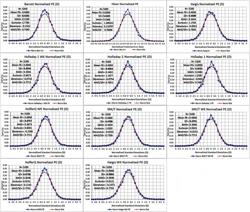
66                                               STATISTICAL ANALYSIS OF SPHERICAL EQUIVALENT

                                                                                                                        Figure 1. A normal probability
                                                                                                                        density distribution (Gaussian)
                                                                                                                        has 68.3% of the data within ±1
                                                                                                                        SD, 95.5% within ±2 SD, and
                                                                                                                        99.7% within ±3 SD.

thickness to show their relationship and effect on PE.                            (ELP) and refraction. Although changes in the SEQ power
Knowledge of the PE distributions is necessary to determine                       (not astigmatic) of the cornea are stable by 3 to 4 months or
the appropriate statistics for comparison of the outcomes                         earlier,changes in the actual ELP, which directly affect the
for formulas, procedures, and devices. We then proposed a                         refraction, are usually not stable until 6 to 12 months
new method for statistical analysis of univariate SEQ PE.                         postoperatively.12–14 The U.S. Food and Drug Adminis-
                                                                                  tration typically requires 12-month studies to assure the
DESIGNING A PROSPECTIVE STUDY                                                     stability of the results. For results to be reliable and re-
Inclusion criteria should include no preoperative or                              fractions stable, the 6-month visit is a good compromise.
postoperative pathology, 1 eye only from each patient, and                        Shorter postoperative periods for reporting results have
corrected visual acuity of greater than or equal 20/30 to                         more variability and lower reliability.
increase the likelihood that the postoperative refraction
sphere and cylinder is accurate to ±0.25 diopters (D) with                        Definitions
vertex distance specified. Multiple contributing surgeons                         The proper statistical analysis of univariate (SEQ) and out-
broaden the applicability of the results. Studies performed                       comes after cataract, refractive, and corneal surgery is chal-
by 1 surgeon have unique factors that can affect the results,                     lenging, even for biostatisticians. The following discourse
including patient population, incision design, IOL insertion                      provides the basis for evaluating PE using the appropriate
and placement, surgical instrumentation, and postoperative                        statistics and explains the interpretation for the reader. The
medications.8,9 In particular, the method of capsulorhexis                        data that are used come from 2 large cataract surgery data-
(eg, manual, femtosecond laser, or Zepto) along with its size                     sets.15 The metric used for determining the accuracy of re-
and location have all been shown to not only affect the                           fractive outcomes is called PE.16 It is the difference in the actual
strength of the bag but also the contraction that occurs                          refraction and the predicted refraction using a specific formula:
postoperatively.10,11 This contraction can cause axial and
lateral displacement of the IOL, which affects the lens                             Prediction Error (D) = Actual SEQ Refraction (D) –
effectivity and the final postoperative effective lens position                   Predicted SEQ Refraction (D)                     (1)

                                                                                                                        Figure 2. Using dataset 1, the
                                                                                                                        distributions of axial length (blue
                                                                                                                        line), SEQ keratometry, anatomic
                                                                                                                        ACD, and CLT along with a normal
                                                                                                                        distribution (red line) (ACD = an-
                                                                                                                        terior chamber depth; CLT = crys-
                                                                                                                        talline lens thickness; MAD = mean
                                                                                                                        absolute deviation; SEQ = spherical
                                                                                                                        equivalent).

Volume 47 Issue 1 January 2021

                Copyright © 2020 Published by Wolters Kluwer on behalf of ASCRS and ESCRS. Unauthorized reproduction of this article is prohibited.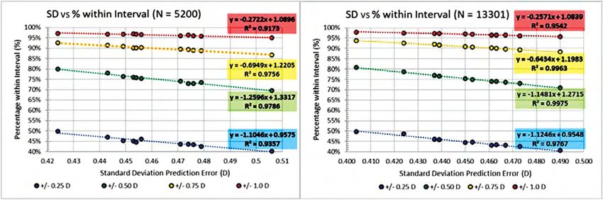
STATISTICAL ANALYSIS OF SPHERICAL EQUIVALENT                                                             67

     Table 1. The 1% and 5% probability points of Gg.
                                                                     Probability Points of Gg
     Size of                          Upper                                                                           Lower
     Sample n’        DOF n*        Limit of Gg     Upper 1%        Upper 5%        Lower 5%         Lower 1%       Limit of Gg     Mean of Gg      SD of Gg
     6                     5           1.000           0.980           0.954           0.696           0.626           0.4472          0.8385        0.0786
     11                   10           1.000           0.941           0.911           0.710           0.656           0.3162          0.8180        0.0613
     16                   15           1.000           0.916           0.891           0.720           0.677           0.2681          0.8113        0.0516
     21                   20           1.000           0.902           0.879           0.728           0.691           0.2236          0.8079        0.0454
     26                   26           1.000           0.892           0.870           0.734           0.701           0.2000          0.8059        0.0410
     31                   30           1.000           0.884           0.864           0.739           0.709           0.1826          0.8046        0.0376
     36                   36           1.000           0.878           0.859           0.743           0.715           0.1690          0.8036        0.0350
     41                   40           1.000           0.873           0.855           0.746           0.720           0.1581          0.8029        0.0328
     46                   45           1.000           0.869           0.851           0.749           0.725           0.1491          0.8023        0.0310
     61                   60           1.000           0.865           0.849           0.751           0.728           0.1414          0.8019        0.0295
     76                   76           1.000           0.863           0.839           0.759           0.741           0.1155          0.8005        0.0242
     101                 100           1.000           0.846           0.834           0.764           0.748           0.1000          0.7999        0.0210
     501                 500           1.000           0.820           0.814           0.783           0.776           0.0447          0.7983        0.0095
     1001                1000          1.000           0.813           0.809           0.787           0.782           0.0316          0.7981        0.0067
*
    Degrees of freedom

   This definition is opposite to what we have defined in                             sum of the prediction errors (PEi) divided by the number
some earlier articles, but agrees with our most recent pub-                           (n) of values in the dataset:
lication.15 We have chosen this definition because when the
                                                                                         Mean PE = x = Sum PEi/n                                             (3)
PE is negative, it is myopic, just similar to the refraction, and
when PE is positive, it is hyperopic. This avoids the problem                           Note that, in Microsoft Excel, the function for the mean is
of the PE having the opposite the sign of the SEQ refraction.                         AVERAGE.
   This definition of PE is true whether the refractions are                            The SD of the PE is the square root of the mean of the sum of
vectors representing an astigmatic refraction or scalar                               the squares (root mean square [RMS]) about the mean of the
values such as the SEQ refraction, but we will limit our                              ðPEi  xÞ values.17 For a normal distribution, 68.3% of data are
current discussion to scalar values. The SEQ refraction is                            within ±1.0 SD, and in Microsoft Excel, the function is STDEV.S:
defined as the sphere plus one half of the cylinder in the                                                qffiffiffiffiffiffiffiffiffiffiffiffiffiffiffiffiffiffiffi2
                                                                                                                      i xÞ
spherocylindrical form or one half of each cylinder in the                              SD of the PE = SumðPE    n1                                (4)
cross-cylinder form as follows:                                                          Another statistical measure of variation is the mean
     SEQ = sphere + ½ cylinder = ½ (cylinder 1 + cylinder 2) (2)                      absolute deviation (MAD). The MAD of the PE is calcu-
                                                                                      lated by taking the mean of the absolute values of the PEi
Statistical Terms                                                                     about the mean. Note that, in Microsoft Excel 2010, the
Mean, SD, Mean Deviation, Median, and Mean Absolute                                   function for the MAD is AVEDEV:
Error Calculating the mean PE is no different than calcu-
lating any other mean. The sample mean is the arithmetic                                 MAD = Sum | PEi  x|/n                                              (5)

Figure 3. A: The correlation of SEQ preoperative refractions and axial lengths for 4710 patients of the 5200 cases, before affected by
cataract. The axial length (blue line) is the primary factor determining the extreme peak of emmetropia (60%, green line). B: The peak for
SEQ preoperative refraction is 8% higher than the axial length peak due to the inverse correlation (black dots) of keratometry and axial
length from 22 to 24.5 mm (AL = axial length; K = keratometry; SEQ = spherical equivalent).

                                                                                                                                 Volume 47 Issue 1 January 2021

              Copyright © 2020 Published by Wolters Kluwer on behalf of ASCRS and ESCRS. Unauthorized reproduction of this article is prohibited.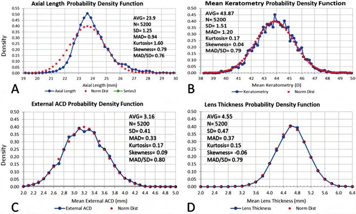
68                                                STATISTICAL ANALYSIS OF SPHERICAL EQUIVALENT

                                                                                                                        Xn         3
                                                                                                               n             xi  x
                                                                                                  G1 ¼                                                 (6)
                                                                                                         ðn  1Þðn  2Þ i¼1     s

                                                                                      If skewness is positive, the data are positively skewed, and
                                                                                   if negative, the data are negatively skewed. A rule of thumb
                                                                                   is that:

                                                                                      1. If skewness is less than 1 or greater than +1, the
                                                                                         distribution is highly skewed.
                                                                                      2. If skewness is between 1 and ½ or between +½
                                                                                         and +1, the distribution is moderately skewed.
                                                                                      3. If skewness is between ½ and +½, the distribution is
                                                                                         approximately symmetric.

                                                                                      Another characteristic of the normal distribution for
Figure 4. The distributions by surgeon of the individual lens con-
stants for both datasets; 81% of dataset 1 and 86% of dataset 2 had                which we can test is kurtosis. In probability theory and
individual surgeon lens constants that were within ±0.10 D of the                  statistics, kurtosis (from Greek: kurtό§, kyrtos or kurtos,
mean.                                                                              meaning curved or arching) is a measure of the tailedness of
                                                                                   the probability distribution of a real-valued random vari-
                                                                                   able. The standard measure of a distribution’s kurtosis,
   For a normal distribution, the MAD is 0.7979 × SD and                           originating with Karl Pearson, is a scaled version of the
comprises 57.51% of the cases.                                                     fourth moment of the distribution.18 This number is related
   Another statistic often reported is the median of the                           to the tails of the distribution, not its peak; hence, the
absolute values (Median in Excel) where the number of                              sometimes-seen characterization of kurtosis as peakedness
values above and below is equal (MedAE). The MedAE is                              is incorrect.19 For this measure, higher kurtosis corre-
0.6745 × SD, where exactly 50% of the absolute values are                          sponds to greater extremity of deviations (or outliers) and
within this value and 50% outside of it.17                                         not the configuration of data near the mean.
   As we have defined earlier, the mean PE x is the ar-                              One measure used for this characteristic is the excess
ithmetic mean of the data. We will see that the datasets                           kurtosis function:
are rarely normal because our goal is to have a PE of zero, so
formulas, procedures, and devices have (1) peaks that are                             g¼m4
                                                                                        m2
                                                                                            3;                                                        (7)
much higher and narrower than a normal distribution and                                       2                                  Pn               4
                                                                                                                                       ðxi xÞ
(2) tails that are usually heavier. The asymmetry or skewness                         where, the fourth moment m4 ¼ i¼1n            and m22 is the
of the PE distribution is usually minimal because the chances                      second moment (variance) squared. By subtracting 3, g is
of myopic or hyperopic PEs are formulated to be equal. Even                        zero for a normal distribution and increases above zero
though the PE distributions are not normal, it will be helpful                     with increasing leptokurtosis. In Excel, the kurtosis func-
to review some of the characteristics of a normal distribution                     tion is KURT.
for comparison.                                                                       Although we will see that none of the formula PE datasets
   Normal Distribution When a probability density dis-                             are normal, we should mention that Shapiro-Wilk test for
tribution is normal (Gaussian) as shown in Figure 1, 68.3%                         univariate normality and the Anderson-Darling test for
of the data are within ±1 SD, 95.5% within ±2 SD, and                              multivariate normality have the best power for a given
99.7% within ±3 SD. Note that, in Microsoft Excel, the                             significance using Monte Carlo simulations. An older test,
function for the SD of a population is STDEV.P.                                    proposed by Geary more than 100 years ago, compares the
                                                                                                 qffiffiffiffiffiffiffi
                                                                                   ratio (Gg) of the MADffi    with the SD.20 The normal value for
Kurtosis, Skew (Asymmetry), and Geary Ratio                                        MAD/SD is 2=p ¼ 0:80, and departure from this value
As stated earlier, the values given for the percentage of cases                    for a given sample size determines the P value for not being
within ±1 SD or for 1 MAD are only true if the distribution                        normal. This ratio is easy to compute, and the values are
is normal. We will see from our analysis of actual datasets                        readily available, so it is a quick way of confirming that the
that the PE distribution is not a normal distribution. There                       distribution is not normal. Table 1 lists the 1% and 5%
are 2 properties of any distribution that are usually tested:                      probability points of the Gg distribution for samples from 6
symmetry (skewness) and kurtosis (tailedness). If the data                         to 1001. We will see that all 11 formulas have PEs for both
are not symmetrical about the mean and have a longer tail                          datasets that are far below the 0.782, indicating they are not
to the right, they are said to be positively skewed (Figure 2, A).                 normal at a P value much less than .01.
By contrast, if the tail to the left is longer, the data are said to be               Distributions of Biometric Measurements–Axial
negatively skewed. The standardized measure for skewness                           Length, Keratometry, Anatomic Anterior Chamber
(G1) for a population in Excel (Skew) and in most modern                           Depth, and Lens Thickness Using dataset 1, the distri-
software packages is the adjusted Fisher-Pearson standardized                      butions of axial length, SEQ keratometry, anatomic anterior
moment coefficient, given by the following formula:                                chamber depth, and crystalline lens thickness along with a

Volume 47 Issue 1 January 2021

                 Copyright © 2020 Published by Wolters Kluwer on behalf of ASCRS and ESCRS. Unauthorized reproduction of this article is prohibited.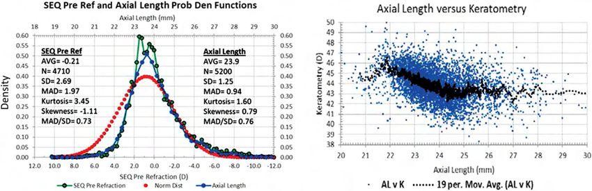
STATISTICAL ANALYSIS OF SPHERICAL EQUIVALENT                                                          69

                                                                                                                        Figure 5. The PEs varied from
                                                                                                                        0.400 to 0.540 D for each surgeon
                                                                                                                        who contributed more than 30
                                                                                                                        cases: SA60AT IOL (A) and
                                                                                                                        SN60WF IOL (B). There was no
                                                                                                                        significant correlation between
                                                                                                                        the number of cases and the SD of
                                                                                                                        the PE or the individual surgeon’s
                                                                                                                        lens constant, although the
                                                                                                                        spread for both decreased as the
                                                                                                                        number of cases contributed in-
                                                                                                                        creased (PE = prediction error).

normal distribution (in red dots) are shown in Figure 2. For                      cases) before affected by cataract. The axial length (blue
reference, a true normal density distribution will have a                         line) is the primary factor determining the extreme peak of
peak (at the mean) of 0.40. Notice that the axial length has a                    emmetropia (60%, green line). The peak for SEQ pre-
narrower, higher peak (0.52) than normal and is skewed to                         operative refraction is 8% higher than the axial length peak
the right (toward longer axial lengths). The other 3 dis-                         due to the inverse correlation (black line) of keratometry
tributions are normal.                                                            and axial length from 22 to 24.5 mm (Figure 3, B). In this
   Figure 3A shows the correlation of SEQ preoperative                            region, as the axial length increases, mean keratometry
refractions and axial lengths (for 4710 patients of the 5200                      decreases, balancing their effects and, thereby, increasing

Figure 6. The actual PE distributions for 11 formulas from the 5200 cases in dataset 1 (blue line) and a normal distribution (red line). The
mean, SD, MAD, kurtosis, skewness, and Geary ratio (MAD/SD) are shown on the inset for each graph (PE = prediction error).

                                                                                                                             Volume 47 Issue 1 January 2021

          Copyright © 2020 Published by Wolters Kluwer on behalf of ASCRS and ESCRS. Unauthorized reproduction of this article is prohibited.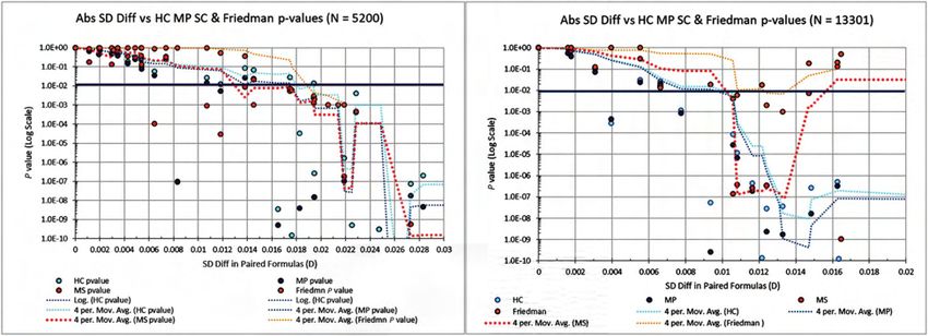
70 STATISTICAL ANALYSIS OF SPHERICAL EQUIVALENT
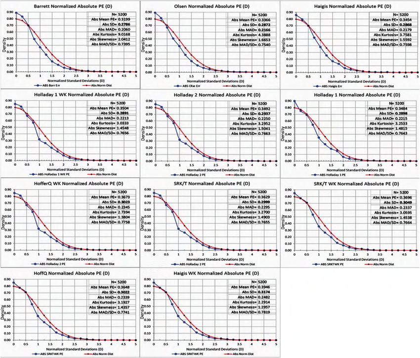
Figure 7. The absolute PE distributions for 11 formulas from the 5200 cases in dataset 1 (blue line) and a normal distribution (red line). The
mean, SD, MAD, kurtosis skewness, and Geary ratio (MAD/SD) are shown on the inset for each graph (PE = prediction error).
the prevalence of emmetropia. Sorsby and Leary and later Lens Constant Optimization
Rubin called this process emmetropization.21,22 The first step in the analysis is to adjust the arithmetic mean
The current emphasis will be restricted to the proper of the PE to zero for each formula by adjusting the lens
statistical methods for comparing means and SDs for PEs constant (to at least to 6 decimal places 0.000000). This
to determine the probabilities of whether values are requires knowledge of which IOLs were implanted in each
different. For example, the statistics could be used to eye and access to the formulas to calculate the predicted
determine if an IOL power calculation formula per- refraction for each patient and to be able to optimize the
formed better than another, a surgical technique was lens constant. In Excel you must have the Add In Analysis
superior to another, or a laser performed better than ToolPak installed; under the Data Tab, there will be a Solver
another. in the Analyze Section. You set the cell with the Target of
Characterizing PE Distributions Over the past 43 years, we the sum of the PEs to zero by changing the cell with the
have been fortunate to have been involved in reporting Lens Constant.
cataract outcomes and have hundreds of datasets with Ideally, although one should optimize the lens constant
the raw data. The most recent publication with Melles for each surgeon in the dataset, the benefit is minimal, and
et al. is representative of the biometry and SEQ PE the effort is much greater. We had 95 surgeons and 127
distributions for 11 formulas.15 Dataset 1 comprised of surgeons in datasets 1 and 2, respectively, with implanta-
5200 single eyes with a spherical IOL (SA60AT), and dataset tion occurring between July 1, 2014, and December 31,
2 comprised of 13 301 single eyes with an aspheric IOL 2015. In dataset 1 the difference in the lens constant by
(SN60WF) for SEQ PE. optimizing all 5200 cases as one surgeon vs each of the 95
Volume 47 Issue 1 January 2021
Copyright © 2020 Published by Wolters Kluwer on behalf of ASCRS and ESCRS. Unauthorized reproduction of this article is prohibited.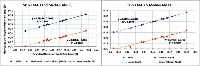
STATISTICAL ANALYSIS OF SPHERICAL EQUIVALENT                                                             71

 Table 2A. Prediction error distribution parameters (N = 5200).
 Formula                         Mean                  SD (D)              ± 1.0 SD (%)             MAD/SD                  Kurtosis                   Skew
 Barrett                         0.000                  0.424                  72.87                  0.755                  2.778                  0.152
 Olsen                           0.000                  0.443                  71.94                  0.761                  1.496                  0.120
 Haigis                          0.000                  0.449                  71.88                  0.768                  1.176                  0.003
 Holladay 1                      0.000                  0.453                  72.08                  0.768                  1.039                  0.043
 Holladay 1 WK                   0.000                  0.454                  72.46                  0.771                  0.947                  0.071
 Holladay 2                      0.000                  0.456                  72.46                  0.765                  1.108                  0.075
 SRK/T                           0.000                  0.471                  71.71                  0.771                  1.020                  0.033
 Hoffer Q                        0.000                  0.474                  70.94                  0.770                  0.974                  0.124
 Hoffer Q WK                     0.000                  0.476                  70.87                  0.771                  0.830                  0.157
 SRK/T WK                        0.000                  0.479                  71.75                  0.772                  0.974                  0.124
 Haigis WK                       0.000                  0.506                  70.04                  0.781                  0.612                  0.107

resulted in SDs of the PE of 0.4726 individually and 0.4791                            1001 cases, so for a normal distribution, there is a 0.01
globally, a difference of 0.0065 D, which is not clinically or                         probability of a value less than 0.782 (bottom of column 7).
statistically significant. Because the difference is negligible,                       We see from Tables 2 and 3 and Figure 4 that all our
it is acceptable to determine a single global lens constant                            formulas are far less than this value and, therefore, not
that optimizes the PE to zero. The distributions by surgeon                            normal. Furthermore, we see that converting to absolute
of the individual lens constants are shown in Figure 4 for                             values exaggerates the kurtosis, introduces significant
both datasets; 81% of dataset 1 and 86% of dataset 2 had                               skewness (asymmetry), and lowers the Geary ratio (Gg)
individual surgeon lens constants that were within ±0.10 D                             even further.
of the mean. The PEs varied from 0.400 to 0.540 D for each                               In these datasets, none of the PE distributions with any
surgeon who contributed more than 30 cases (Figure 5).                                 formula are normal. The peak is always higher than a
There was no significant correlation between the number of                             normal distribution, and the tails are always heavier
cases and the SD of the PE or the individual surgeon’s lens                            (higher). The distributions (not absolute) are very sym-
constant, although the spread for both decreased as the                                metrical with skewness values within ±0.50 D. It is not
number of cases contributed increased.                                                 surprising that the peaks are higher than normal. The goal
   Figure 6 shows the actual PE distributions for 11 for-                              of an IOL calculation formula is to have a PE of zero: a
mulas from the 5200 cases in dataset 1 in blue and a normal                            perfect formula would have a 100% peak at zero. The better
distribution in red. The mean, SD, MAD, kurtosis, skew-                                the formula, the closer it is to that goal.
ness, and Geary ratio (MAD/SD) are shown on the inset for                                However, in the absolute distributions in Figure 7, the
each graph.                                                                            higher peak and tails are due to moving some of the in-
   Figure 7 shows the absolute PE distributions for 11                                 termediate PEs (1.0 to 3.0 SDs) to the peak and the re-
formulas from the 5200 cases in dataset 1 in blue and a                                mainder to the tails. In Figures 6 and 7, the area below the
normal distribution in red. The mean, SD, MAD, kurtosis                                red line (normal distribution) must equal the area above the
skewness, and Geary ratio (MAD/SD) are shown on the                                    red line because the area under the probability curve must
inset for each graph.                                                                  be 1.0 for both the blue and red curves.
   From Table 1, by taking the ratio of the MAD/SD (Gg),                                 In Table 4, we can see the exact amounts that have been
one might determine whether a dataset is not normal at the                             moved for each interval of the SDs for dataset 2 (N = 13 301).
1% probability. In both datasets, we have well more than                               The cases within ±1 SD for all formulas are higher than the

 Table 2B. Absolute prediction error distribution parameters (N = 5200).
                                                    Median                                                                         MAD/
 Formula            Mean      SD (D)     MAD (D)    Abs (D)     ± 0.25 D (%)    ± 0.50 D (%)     ± 0.75 D (%)    ± 1.00 D (%)        SD      Kurtosis     Skew

 Barrett            0.320     0.279       0.206      0.252          49.8            80.0             92.7            97.2          0.739       9.017      2.041
 Olsen              0.337     0.287       0.217      0.268          47.1            78.0             91.5            96.7          0.754       4.389      1.665
 Haigis             0.345     0.287       0.218      0.278          45.3            76.3             90.9            96.8          0.760       3.758      1.559
 Holladay 1         0.348     0.290       0.222      0.281          45.1            75.9             90.1            96.9          0.764       3.253      1.482
 Holladay 1
   WK               0.350     0.289       0.221      0.283          44.6            75.8             90.1            96.8          0.766       3.033      1.455
 Holladay 2         0.349     0.294       0.225      0.277          46.1            75.3             90.4            96.6          0.766       3.295      1.504
 SRK/T              0.363     0.300       0.230      0.290          43.7            74.1             89.5            96.0          0.765       3.270      1.490
 Hoffer Q           0.365     0.302       0.234      0.292          43.7            73.0             89.4            96.3          0.774       3.193      1.436
 Hoffer Q WK        0.367     0.302       0.234      0.295          43.4            72.9             89.0            96.0          0.776       2.739      1.380
 SRK/T WK           0.370     0.305       0.234      0.298          42.4            73.5             88.8            95.9          0.766       3.059      1.454
 Haigis WK          0.395     0.317       0.248      0.321          40.3            69.6             86.8            95.0          0.782       2.291      1.296

                                                                                                                                 Volume 47 Issue 1 January 2021

              Copyright © 2020 Published by Wolters Kluwer on behalf of ASCRS and ESCRS. Unauthorized reproduction of this article is prohibited.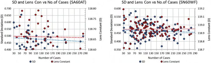
72                                                STATISTICAL ANALYSIS OF SPHERICAL EQUIVALENT

 Table 3A. Prediction error distribution parameters (N = 13 301).
 Formula                      Mean                  SD (D)              ± 1.0 SD (%)             MAD/SD                    Kurtosis                 Skew
 Barrett                      0.000                  0.404                   71.6                  0.770                    1.192                 0.012
 Olsen                        0.000                  0.424                   71.7                  0.767                    1.274                  0.146
 Haigis                       0.000                  0.437                   70.9                  0.773                    1.063                  0.067
 Holladay 1 WK                0.000                  0.439                   70.6                  0.774                    0.956                 0.055
 Holladay 2                   0.000                  0.450                   70.7                  0.778                    0.858                 0.050
 Holladay 1                   0.000                  0.453                   70.7                  0.775                    0.926                  0.036
 Hoffer Q WK                  0.000                  0.461                   70.4                  0.781                    0.747                 0.129
 SRK/T                        0.000                  0.463                   70.4                  0.778                    0.834                 0.080
 SRK/T WK                     0.000                  0.467                   70.5                  0.777                    0.817                 0.056
 Hoffer Q                     0.000                  0.473                   70.3                  0.780                    0.687                 0.071
 Haigis WK                    0.000                  0.490                   70.0                  0.782                    0.688                 0.017

normal, ranging from a high of 3.46% (formula 2) to a                                  When analyzing data of the first type, where, for example,
low of 1.72% for formula 11 (first column). Those cases                             the PE of IOL calculation formulas in the same group is the
came from the 1 to 3 SDs that are all negative (lower than                          random variable used to assess the performance, we will
the normal). The cases with a PE above 3 SD are above                               show that using the SD of PE is the single, most accurate
the normal (positive), which explains why the distri-                               assessment of performance and accurately predicts other
butions are considered heavy tailed. Notice in the last                             measures such as the percentage of cases within an interval
column that the sum in each row of the percentages of                               (eg, ±0.50), the MAD, and the median. We will also provide
variations of the distributions from normal is zero for                             the appropriate, contemporary methods of determining the
each formula.                                                                       whether the performance differences in the SDs are sta-
                                                                                    tistically significant.
STATISTICAL COMPARISON OF PE FOR IOL                                                   As shown in Equation 4, the SD is the square root of the
POWER CALCULATION FORMULAS                                                          mean of the sum of the squares (RMS) divided by the mean.
There are 2 main types of statistical comparison we will                            The RMS value is used throughout science in every dis-
consider: (1) dependent paired samples from the same                                cipline to accurately compare differences in complex
group and (2) independent samples that are from 2 dif-                              shapes, surfaces, or waveforms. In electrical engineering,
ferent groups. The typical comparison of the power cal-                             the energy of an alternating sinusoidal current can be
culation formulas is the first type, which involves the use of                      compared with the energy of a constant direct current using
1 dataset for which the actual refraction is compared with                          the RMS value. The energy of a sinusoid with amplitude of 1
the predicted refraction for each formula. Because only 1                           has an RMS value of 70.7% of its peak and is equal in energy
dataset is used for all formulas, the comparisons are paired                        to the DC value of this amplitude. A perfect wavefront is a
dependent samples for which the PEs for 2 formulas are                              circular flat disk, but the ocular wavefront of the human eye
used for each patient.                                                              is irregular and looks similar to a deformed potato chip. By
   The second type of comparison of independent samples                             computing the RMS value of the deviations from the perfect
from 2 different groups might be comparisons of 2 different                         disc, we find a mean value of 0.38 ± 0.14 mm in the normal
IOLs, surgical techniques, or devices such as femtosecond                           human.23 Even though every human has a unique wave-
laser vs manual capsulorhexis. When independent, the                                front, the RMS value can be used to compare the visual
samples should be randomized and might be slightly dif-                             quality between individuals with different wavefronts. In
ferent in the total number of cases.                                                statistics, the RMS value about the mean is the SD. It allows

 Table 3B. Absolute prediction error distribution parameters (N = 13 301).
                                                 Median                                                                       MAD/
 Formula          Mean     SD (D)     MAD (D)    Abs (D)     ± 0.25 D (%)   ± 0.50 D (%)    ± 0.75 D (%)    ± 1.00 D (%)        SD       Kurtosis      Skew

 Barrett          0.311    0.258       0.197      0.252         49.8            80.8            93.7            97.8          0.762       3.883        1.550
 Olsen            0.325    0.272       0.208      0.258         48.8            78.7            92.5            97.4          0.762       3.975        1.578
 Haigis           0.338    0.277       0.212      0.275         46.1            77.0            91.9            97.3          0.767       3.697        1.504
 Holladay 1 WK    0.340    0.277       0.214      0.275         45.9            76.6            91.7            97.2          0.771       3.360        1.459
 Holladay 2       0.350    0.283       0.218      0.287         44.5            75.4            90.9            97.0          0.770       3.117        1.425
 Holladay 1       0.351    0.287       0.221      0.285         44.7            75.0            90.7            96.8          0.771       3.204        1.445
 Hoffer Q WK      0.360    0.288       0.223      0.295         43.1            74.0            90.2            96.5          0.774       2.856        1.375
 SRK/T            0.360    0.291       0.225      0.292         43.3            74.0            90.0            96.5          0.774       3.082        1.408
 SRK/T WK         0.363    0.294       0.227      0.295         43.1            73.6            89.7            96.5          0.775       3.001        1.395
 Hoffer Q         0.369    0.296       0.230      0.303         42.5            73.0            89.3            96.1          0.776       2.601        1.347
 Haigis WK        0.383    0.305       0.237      0.318         40.6            71.0            88.3            95.6          0.777       2.744        1.342

Volume 47 Issue 1 January 2021

                 Copyright © 2020 Published by Wolters Kluwer on behalf of ASCRS and ESCRS. Unauthorized reproduction of this article is prohibited.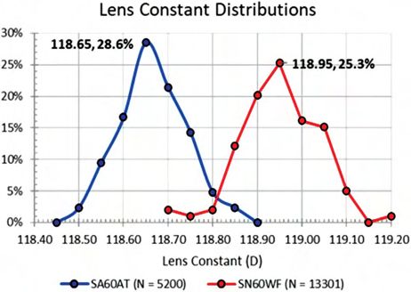
STATISTICAL ANALYSIS OF SPHERICAL EQUIVALENT                                                          73

 Table 4. Difference from normal distribution (N = 13 301).
                                                                                   comparing the variances of 2 dependent variables can be
                                                                                   improved by using the heteroscedastic (HC) method, a
                                                                                   simple extension of the Morgan-Pitman test to the
                                                                                   Spearman modification of the Morgan-Pitman test.25 It is
                                                                                   based partly on a HC method for making inferences about
                                                                                   Pearson correlation.26
                                                                                      Performing these calculations is not practical for most
                                                                                   clinicians, but fortunately, open access software is available
                                                                                   from The R Project for Statistical Computing. Figure 8
                                                                                   shows, for the datasets 1 and 2 comprising 5200 and 13 301
                                                                                   eyes, the P values for each pair of variances for the 11
                                                                                   formulas for (1) the HC method, (2) the older Morgan-
                                                                                   Pitman test based on Pearson correlation (MP), (3) the
                                                                                   modification of the Morgan-Pitman suggested by
                                                                                   McCulloch (1987) where Pearson correlation is replaced by
                                                                                   Spearman correlation (SC), and (4) the Friedman test with
comparison of different shaped probability distributions                           the Nemenyi post hoc analysis used on the absolute
with a single number.                                                              values.27–29 In Figure 8, we see that the Friedman test with
  For any probability density distribution, the total area                         the Nemenyi post hoc analysis using the absolute values for
under the curve is 1. The argument that the SD weighs the                          the PE (yellow points) results in much higher P values,
cases by the square of values is not true; on the contrary, it                     especially when the paired formula SDs differences are
takes the square root of the mean of the sum of the squares so                     lower. We also see that, in dataset 2 with 13 301 cases, the
that the values are appropriately weighted and the area under                      Friedman P value goes back up at the higher values (have an
the curve is 1. For a normal distribution, the ratio of the                        inflection). The cause of the erratic P values with the
MAD/SD is 0.80, so the MAD is only 20% less than the SD.                           Friedman test is due primarily to the asymmetrical shape of
  Perhaps even more important is that the variance of the                          the absolute values, the improper weighting of the values
random variable (PE) can be expressed as a function of the                         using the absolute values, and the post hoc analysis in the
variances and covariances of its constituent pieces (axial                         presence of heavy tails (Figure 7). Hoffer et al. had rec-
length, keratometry, predicted ELP, and pupil size).24                             ommended the bootstrap method to deal with certain issues
Norrby identified 9 parameters that contributed more                               with datasets.1 However, the erratic nature of the P values is
than 1% to the total PE, with the ELP accounting for 35%, the                      exactly why Athreya states, “Unless one is reasonably sure
postoperative refraction 27%, the axial length 17%, corneal                        that the underlying distribution is not heavy tailed, one
power 11%, and the pupil size 8% of the total PE. With other                       should hesitate to use the naive bootstrap (post hoc
measures such as MAD and median, such an analysis is not                           analysis).”30 For the methods using the SD (HC, MP, and
possible because the total is not equal to the sum of the parts.                   SC), there is no reversal of the P values. The superiority of
  Because the PE measures are (1) dependent and (2) not                            the HC method over the MP and SC methods becomes
normal, the standard F test for comparing SDs can not be                           more apparent the smaller the sample size.25 The original
used. It requires independence and normality. New per-                             Morgan-Pitman test is based in part on testing the hy-
spectives in statistics have shown that, when not normal                           pothesis of a zero Pearson correlation. The conventional
distributions are fairly symmetrical and heavy tailed,                             method assumes homoscedasticity. As we move toward

 Table 5. Matrix of paired standard deviation differences for dataset 1 (N = 5200).
                           SD       SD       SD         SD              SD             SD         SD         SD             SD             SD       SD
 Formula          SD       Dif      Dif      Dif        Dif             Dif            Dif        Dif        Dif            Dif            Dif      Dif
 Barrett        0.424    0.000
 Olsen          0.443    0.018     0.000
 Haigis         0.449    0.025     0.006    0.000
 Holladay 1     0.453    0.029     0.011    0.004      0.000
 Holladay 1     0.454    0.030     0.012    0.005      0.001          0.000
   WK
 Holladay 2     0.456    0.032     0.014    0.007    0.003         0.002      0.000
 SRK/T          0.471    0.047     0.028    0.022    0.018         0.017      0.015    0.000
 Hoffer Q       0.474    0.050     0.031    0.025    0.021         0.019      0.017    0.003               0.000
 Hoffer Q WK    0.476    0.051     0.033    0.027    0.023         0.021      0.019    0.005               0.002          0.000
 SRK/T WK       0.479    0.055     0.037    0.030    0.026         0.025      0.023    0.008               0.005          0.003      0.000
 Haigis WK      0.506    0.082     0.064    0.057    0.053         0.052      0.050    0.036               0.033          0.031      0.027    0.000
                         Barrett   Olsen    Haigis Holladay 1 Holladay 1 WK Holladay 2 SRK/T              Hoffer Q     Hoffer Q WK SRK/T WK Haigis WK

                                                                                                                              Volume 47 Issue 1 January 2021

           Copyright © 2020 Published by Wolters Kluwer on behalf of ASCRS and ESCRS. Unauthorized reproduction of this article is prohibited.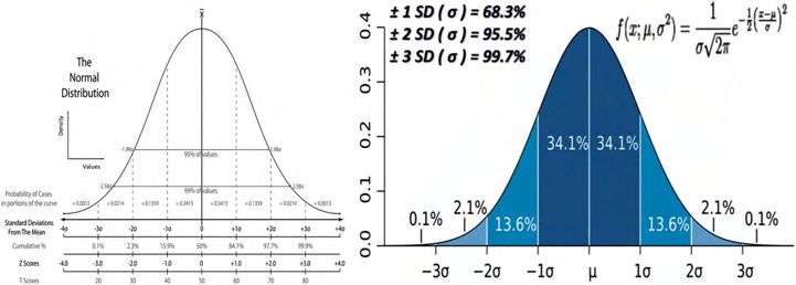
74                                                STATISTICAL ANALYSIS OF SPHERICAL EQUIVALENT

 Table 6. Matrix of paired adjusted HC P values for dataset 1 (N = 5200).

HC = heteroscedastic; Shaded Boxes = P value > 0.05 and are not considered statistically significant.

heavy-tailed distributions, heteroscedasticity becomes an                          performed. The older Bonferroni correction can be criti-
issue. In effect, an incorrect estimate of the standard error is                   cized for being overly conservative, thus potentially ex-
being used. The HC method addresses this problem. The                              cluding results of real significance.31,32 The adjusted P values
SD is not only the best random variable to use statistically                       should be the values reported.
but also accurately predicts other key metrics. The first                             In Table 5, for dataset 1 (N = 5200), the smallest differences
relationship that the SD accurately predicts is the per-                           in SD correspond roughly with the 19 highest adjusted
centage of cases within various intervals, such as within                          P values in Table 6 (pink-shaded boxes) that are above 0.05
±0.25, ±0.50, ±0.75, and ±1.00 D as shown in Figure 9.                             and are not considered statistically significant. The adjusted
   The R2 values are extremely high, ranging from 0.9173 to                        P values along the diagonal are 1.0 because the probability of
0.9975. The SD also predicts the MAD and median even                               a formula being the same as itself is 1.0. For dataset 2
more accurately as shown in Figure 10, with the R2 values                          (N = 13 301), because the sample size was much larger, there
are above 0.976. Table 5 summarizes the differences in each                        were only 2 pairs of adjusted P values above 0.05.
pair (55) of the SDs for the 11 formulas. The differences in
SD for the 11 formulas range from a low of 0.001 D to a high                       DETERMINING MODIFIED MP P VALUE OF 2 SDS
of 0.082 D. The corresponding adjusted P values using the                         FOR 2 INDEPENDENT DATASETS
HC method are tabulated in Table 6. The P values have                              The second type of statistical comparison using 2 or more
been adjusted because we conducted multiple comparisons                            independent datasets would be used to compare the aspheric
on the same dependent variable with the 11 formulas. The                           (13 301) and nonaspheric (5200) IOLs. A generalization of
chance of committing a type I error increases with multiple                        the HC version of the Morgan-Pitman test based on Pearson
comparisons, thus increasing the likelihood of determining                         correlation (MP) is used.26,27 The aspheric IOL with 13 301
a significant result by pure chance. To correct for this and                       cases that reflects current aspheric IOLs has a lower SD
protect from type I errors, the Holm correction has been                           (0.404 D) than the nonaspheric IOL (0.424 D) with 5200

Figure 8. The Friedman test with the Nemenyi post hoc analysis using the absolute values for the PE (yellow points) results in much higher P values,
especially when the paired formula SDs differences are lower. In dataset 2 with 13 301 cases, the Friedman P value goes back up at the higher values
(has an inflection) (HC = heteroscedastic; MP = the older Morgan-Pitman test based on Pearson correlation; SC = Spearman correlation).

Volume 47 Issue 1 January 2021

                 Copyright © 2020 Published by Wolters Kluwer on behalf of ASCRS and ESCRS. Unauthorized reproduction of this article is prohibited.
STATISTICAL ANALYSIS OF SPHERICAL EQUIVALENT 75
Figure 9. The SD accurately predicts the percentage of cases within various intervals, such as ±0.25, ±0.50, ±0.75, and ±1.00 D: dataset 1 (A)
and dataset 2 (B). The R2 values are extremely high, ranging from 0.9173 to 0.9975.
cases and a more accurate PE as predicted by Norrby.24 The minimal standard. The best way of determining a mini-
difference in SDs of 0.02 D results in 80.8% of PEs within mum sample size for statistical significance is empirically
±0.50 D with the aspheric IOL vs 79.8% with the nona- from previous studies. In Figure 8, dataset 1 with 5200 cases
spheric, a difference of 1.0% (P = .005). The smaller PE of the was able to show a difference of 0.02 D at a P value of 0.01
aspheric IOL is a result of the reduction in ocular spherical and dataset 2 with 13 301 cases was able to show a dif-
aberration. This reduction of spherical aberration reduces ference of 0.007 D at a P value of 0.01. Using the datasets 1
the influence of the pupil size on the effective IOL power for and 2, we can use sequentially ordered sampling to reduce
an individual patient and improves the quality of vision.24,33 the size of the sample and compute the HC P value.
In fact, Norrby predicted in 2008 that the pupil size would be Figure 11 shows the number of cases and the resulting P
8% of the SD, and we found it to be 5% (0.02/0.40). values. The number of cases to achieve the same level of the
If there were more than 2 independent random variables difference in the SDs of 0.02 D for P value of approximately
compared (3 or more IOLs), the P values must be adjusted 0.01 for both datasets is between 300 and 700.
because we conducted multiple comparisons on the same In this article, we have discussed the key elements for de-
independent random variable (IOL type in this case) and scribing and analyzing the accuracy of IOL calculation for-
the chance of committing a type I error increases. The mulas. We have (1) outlined the criteria for patient and data
Holm, Hommel, and Hochberg methods all represent a inclusion, (2) recommended the appropriate sample size, (3)
better balance excluding spurious positives without ex- reinforced the requirement that the formulas be optimized to
cluding true positives than the Bonferroni.31,32,34,35 bring the mean error to zero, (4) demonstrated why the SD is
the single best parameter to characterize the performance of an
Minimum Sample Size for Statistical Significance IOL power calculation formula; it determines the percentage of
A statistical significance with a P value of 0.01 is usually cases within a given interval, the MAD, and the median of the
considered excellent and 0.05 is acceptable as a scientific absolute values; and (5) proposed that the HC statistical
Figure 10. The SD also predicts the MAD and median even more accurately with the R2 values are above 0.976 (AE = absolute error; PE =
prediction error).
Volume 47 Issue 1 January 2021
Copyright © 2020 Published by Wolters Kluwer on behalf of ASCRS and ESCRS. Unauthorized reproduction of this article is prohibited.76 STATISTICAL ANALYSIS OF SPHERICAL EQUIVALENT
Figure 11. Graph showing that the number of cases to achieve a P value of .01 for an SD difference of 0.02 D in dataset 1 (A) is 300 and for an
SD difference 0.007 D in dataset 2 (B) is 2000 (HC = heteroscedastic).
method is the preferred method of analysis, especially for 2. Aristodemou P, Cartwright NEK, Sparrow JM, Johnston RL. Statistical
analysis for studies of intraocular lens formula accuracy. Am J Ophthalmol
smaller datasets; it is much better at controlling the probability 2015;160:1085–1086
of a type I error when the marginal distributions have heavy 3. Wilcoxon F. Individual comparisons by ranking methods (PDF). Biometrics
tails but are still symmetric. Details for downloading the open 1945;1:80–83
4. Friedman M. The use of ranks to avoid the assumption of normality implicit in
access software from The R Project for Statistical Computing the analysis of variance. J Am Stat Assoc 1937;32:675–701
can be found at https://www.r-project.org/ and details re- 5. Friedman M. A correction: the use of ranks to avoid the assumption of
garding how to implement HC analysis are in the README normality implicit in the analysis of variance. J Am Stat Assoc 1939;34:
109
files at https://osf.io/nvd59/quickfiles.
6. Benavoli A, Corani G, Mangili F. Should we really use post-hoc tests based
on mean-ranks? J Mach Learn Res 2016;17:1–10
7. Hoffer KJ, Aramberri J, Haigis W, Olsen T, Savini G, Shammas HJ, bentow
S. Reply: to PMID 26117311. Am J Ophthalmol 2015;160:1086–1087
WHAT WAS KNOWN 8. Holladay JT, Prager TC, Ruiz RS, Lewis JW, Rosenthal H. Improving the
Prediction error in diopters, the difference between the SEQ predictability of intraocular lens power calculations. Arch Ophthalmol 1986;
104;539–541
of the actual and predicted refraction, is used to measure the
9. Holladay JT, Prager TC, Chandler TY, Musgrove KH, Lewis JW, Ruiz RS. A
accuracy of intraocular lens power calculation formulas. three-part system for refining intraocular lens power calculations. J Cataract
The prediction error is usually converted to absolute values, Refract Surg 1988;14:17–24
creating a random variable that is not normal, asymmetric, 10. Findl O, Hirnschall N, Draschl P, Wiesinger J. Effect of manual capsulorhexis
and heavy tailed; the formulas are then compared using size and position on intraocular lens tilt, centration, and axial position.
decades-old statistical methods that are erratic and unreli- J Cataract Refract Surg 2017;43:902–908
11. Toto L, Mastropasqua R, Mattei PA, Agnifili L, Mastropasqua A, Falconio G,
able for predicting the P values for a type 1 error.
Nicola MD, Mastropasqua L. Postoperative IOL axial movements and re-
Other measures such as mean absolute deviation, median
fractive changes after femtosecond laser-assisted cataract surgery versus
absolute error, mean absolute error, and percentages within conventional phacoemulsification. J Refractive Surg 2015;31:524–530
various dioptric intervals are often reported to ameliorate this 12. Caglar C, Batur M, Eser E, Demir H, Yaşar T. The stabilization time of ocular
variability and limitation when using absolute values, but they measurements after cataract surgery. Semin Ophthalmol 2017;32:412–417
also do not eliminate the problem. 13. de Juan V, Herreras JM, Pérez I, Morejón Á, Rı́o-Cristóbal A, Martı́n R,
Fernández I, Rodrı́guez G. Refractive stabilization and corneal swelling
WHAT THIS PAPER ADDS after cataract surgery [published correction appears in Optom Vis Sci.
2013 Apr;90(4):e134. Cristóbal, Ana Rı́o-San [corrected to Rı́o- Cristóbal,
The original, signed prediction error is the random variable
Ana]]. Optom Vis Sci 2013;90:31–36
that is not normal, symmetric, and heavy tailed. 14. Gray A. Modern Differential Geometry of Curves and Surfaces. Boca Raton,
The SD is the single most accurate measure of prediction FL: CRC Press; 1993:375–387;279–285
error when comparing intraocular lens power calculation 15. Melles RB, Holladay JT, Chang WJ. Accuracy of intraocular lens calculation
formulas; it predicts the results with other measures such as formulas. Ophthalmology 2018;125:169–178
those mentioned earlier with extremely high R2 values ranging 16. Holladay JT, Moran JR, Kezirian GM. Analysis of aggregate surgically
induced refractive change, prediction error, and intraocular astigmatism.
from 0.9173 to 0.9975.
J Cataract Refract Surg 2001;27:61–79
The SD of the prediction error allows the use of modern,
17. Remington RD, Schork MA. Statistics with Applications to the Bilogical
contemporary heteroscedastic statistical methods spe- and Health Sciences. Englewood Cliffs, NJ: Prentice-Hall Inc; 1970;
cifically intended for use with not normal, symmetric, 32–36
heavy tailed random variables, providing accurate P val- 18. Zenga M, Fiori A. Karl Pearson and the origin of kurtosis. Int Stat Rev 2009;
ues for type 1 errors and a valid method for comparing the 77:40–50
formulas. 19. Westfall PH. Kurtosis as peakedness, 1905—2014. R.I.P. Am Stat 2014;
68:191–195
20. Geary RC. The ratio of the mean deviation to the standard deviation as a test
of normality. Biometrika 1935;27:310–332
REFERENCES 21. Sorsby A, Leary GA. A longitudinal study of refraction and its components
1. Hoffer KJ, Aramberri J, Haigis W, Olsen T, Savini G, Shammas HJ, Bentow during growth. Spec Rep Ser Med Res Counc (G B) 1969;309:1–41
S. Protocols for studies of intraocular lens formula accuracy. Am J Oph- 22. Rubin ML. Optics for Clinicians. 2nd ed. Gainesville, FL: Triad Scientific
thalmol 2015;160:403–405.e1 Publishers; 1974:129
Volume 47 Issue 1 January 2021
Copyright © 2020 Published by Wolters Kluwer on behalf of ASCRS and ESCRS. Unauthorized reproduction of this article is prohibited.STATISTICAL ANALYSIS OF SPHERICAL EQUIVALENT 77
23. McCormick GJ, Porter J, Cox IG, MacRae S. Higher-order aberrations in 33. Holladay JT, Piers PA, Koranyi G, van der Mooren M, Norrby NE. A new
eyes with irregular corneas after laser refractive surgery. Ophthalmology intraocular lens design to reduce spherical aberration of pseudophakic
2005;112:1699–1709 eyes. J Refract Surg 2002;18:683–691
24. Norrby S. Sources of error in intraocular lens power calculation. J Cataract 34. Hommel G. A stagewise rejective multiple test procedure based on a
Refract Surg 2008;34:368–376 modified Bonferroni test. Biometrika 1988;75:383–386
25. Wilcox RR. Comparing the variances of two dependent variables. J Stat 35. Hochberg Y. A sharper Bonferroni procedure for multiple tests of signifi-
Distributions Appl 2015;2:7 cance. Biometrika 1988;75:800–802
26. Wilcox RR. Introduction to Robust Estimation and Hypothesis Testing. 5th
ed. San Diego, CA: Academic Press; (in Press)
27. Morgan WA. A test for the significance of the difference between two Disclosures: None of the authors have a financial or proprietary
variances in a sample from a normal bivariate population. Biometrika 1939; interest in any material or method mentioned.
31:13–19
28. Pitman EJG. A note on normal correlation. Biometrika 1939;31:9–12
29. McCulloch CE. Tests for equality of variance for paired data. Commun Stat
Theor Methods 1987;16:1377–1391 First author:
30. Athreya KB. Bootstrap of the mean in the infinite variance case. Ann Stats Jack T. Holladay, MD, MSEE
1987;15:724–731
31. Holm S. A simple sequentially rejective multiple test procedure. Scand J Stat Department of Ophthalmology, Baylor
1979;6:65–70 College of Medicine, Houston, Texas
32. Bonferroni CE. Teoria statistica delle classi e calcolo delle probabilità.
Florence, Italy: Pubblicazioni del R Istituto Superiore di Scienze Economiche
e Commerciali di Firenze. 1936;8:3–62
Volume 47 Issue 1 January 2021
Copyright © 2020 Published by Wolters Kluwer on behalf of ASCRS and ESCRS. Unauthorized reproduction of this article is prohibited.You can also read