Seismicity characterization of oceanic earthquakes in the Mexican territory - Solid Earth
←
→
Page content transcription
If your browser does not render page correctly, please read the page content below
Solid Earth, 11, 791–806, 2020
https://doi.org/10.5194/se-11-791-2020
© Author(s) 2020. This work is distributed under
the Creative Commons Attribution 4.0 License.

Seismicity characterization of oceanic earthquakes
in the Mexican territory
Quetzalcoatl Rodríguez-Pérez1,2 , Víctor Hugo Márquez-Ramírez2 , and Francisco Ramón Zúñiga2
1 Consejo   Nacional de Ciencia y Tecnología, Dirección Adjunta de Desarrollo Científico, 03940, Mexico City, Mexico
2 Centro   de Geociencias, Universidad Nacional Autónoma de México, Juriquilla, Querétaro, Mexico

Correspondence: Quetzalcoatl Rodríguez-Pérez (quetza@geociencias.unam.mx)

Received: 21 November 2019 – Discussion started: 14 January 2020
Revised: 23 March 2020 – Accepted: 2 April 2020 – Published: 5 May 2020

Abstract. We analyzed the seismicity of oceanic earthquakes       1   Introduction
in the Pacific oceanic regime of Mexico. We used data from
the earthquake catalogues of the Mexican National Service
(SSN) and the International Seismological Centre (ISC) from       Mid-ocean ridges and transform fault zones are two of the
1967 to 2017. Events were classified into two different cat-      main morphological features of oceanic environments. Most
egories: intraplate oceanic (INT) and transform fault zone        of the oceanic earthquakes take place in areas close to the
and mid-ocean ridges (TF-MOR) events, respectively. For           active spreading ridges where the seismogenic zone is nar-
each category, we determined statistical characteristics such     row. For this reason, large aspect ratios are often required
as magnitude frequency distributions, the aftershocks decay       to generate moderate-size strike-slip oceanic earthquakes.
rate, the nonextensivity parameters, and the regional stress      Nevertheless, the rupture process of oceanic events is still
field. We obtained b values of 1.17 and 0.82 for the INT          poorly understood. Previous studies showed that these types
and TF-MOR events, respectively. TF-MOR events also ex-           of events have peculiar characteristics. For example, esti-
hibit local b-value variations in the range of 0.72–1.30. TF-     mates of seismic coupling for oceanic transform faults in-
MOR events follow a tapered Gutenberg–Richter distribu-           dicate that about three-fourths of the accumulated moment
tion. We also obtained a p value of 0.67 for the 1 May 1997       is released aseismically (Abercrombie and Ekström, 2003;
(Mw = 6.9) earthquake. By analyzing the nonextensivity pa-        Boettcher and Jordan, 2004), and some oceanic events ex-
rameters, we obtained similar q values in the range of 1.39–      hibit slow slip ruptures (Kanamori and Stewart, 1976; Okal
1.60 for both types of earthquakes. On the other hand, the        and Stewart, 1992; McGuire et al., 1996). Earthquakes that
parameter a showed a clear differentiation, being higher for      have longer durations than those predicted by scaling rela-
TF-MOR events than for INT events. An important implica-          tionships are considered as slow (Abercrombie and Ekström,
tion is that more energy is released for TF-MOR events than       2003). These “slow” ruptures are mainly interpreted as hav-
for INT events. Stress orientations are in agreement with geo-    ing low rupture velocities. On the other hand, others pro-
dynamical models for transform fault zone and mid-ocean           posed that the slow ruptures may be explained as numerical
ridge zones. In the case of intraplate seismicity, stresses are   artifacts generated by the inversion procedures (e.g., Aber-
mostly related to a normal fault regime.                          crombie and Ekström, 2001, 2003). Several oceanic strike-
                                                                  slip events were reported as being energy deficient at high
                                                                  frequencies (Beroza and Jordan, 1990; Stein and Pelayo,
                                                                  1991; Ihmlé and Jordan, 1994) or having high apparent
                                                                  stresses (Choy and Boatwright, 1995; Choy and McGarr,
                                                                  2002). On another front, oceanic earthquakes also occur as
                                                                  intraplate events but to a lesser extent. The reason is that the
                                                                  oceanic plate interiors do not experience significant strain
                                                                  over long periods of time (Bergman and Solomon, 1980;

Published by Copernicus Publications on behalf of the European Geosciences Union.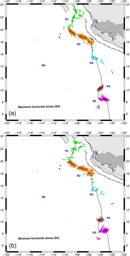
792                                             Q. Rodríguez-Pérez et al.: Seismicity characterization of oceanic earthquakes

Bergman, 1986). Oceanic intraplate earthquakes originate
from the following processes: stresses of the oceanic crust,
in regions that concentrate significant deformation; reactiva-
tion of faults; or thermoelastic stresses (Bergman, 1986).
   From the statistical perspective, previous studies showed
that the magnitudes of the major events in the mid-oceanic
ridges and transform fault zones are relatively smaller (6.0 ≤
Mw ≤ 7.2) compared to continental events. The b value in
oceanic environments showed significant variability. For ex-
ample, Tolstoy et al. (2001) reported high b values (b ∼ 1.5)
in the Gakkel Ridge associated with volcanic activity. In
the Southwest Indian Ridge, Läderach (2011) found b val-
ues of about 1.28. Bohnenstiehl et al. (2008) quantified the
b value in the East Pacific Rise, obtaining estimations in the
range of 1.10
Q. Rodríguez-Pérez et al.: Seismicity characterization of oceanic earthquakes 793
Table 1. Major oceanic earthquakes in Mexico (M>6.8).
Event Date Time Long Lat Ms Mw M0 Reference
(dd/mm/yyyy) (hh:mm:ss) (◦ ) (◦ ) (Nm)
1 14/01/1899 02:36:00 −110.00 20.00 7.0 (1)
2 17/12/1905 05:27:00 −113.00 17.00 7.0 7.0 4.40 × 10¹⁹ (2)
3 10/04/1906 21:18:00 −110.00 20.00 7.1 7.1 6.20 × 10¹⁹ (2)
4 31/10/1909 10:18:00 −105.00 8.00 6.9 (3)
5 31/05/1910 04:54:00 −105.00 10.00 7.0 (3)
6 29/10/1911 18:09:00 −101.00 11.00 6.8 (3)
7 16/11/1925 11:54:00 −107.00 18.00 7.0 (4)
8 28/05/1936 18:49:01 −103.60 10.10 6.8 (3)
9 30/06/1945 05:31:21 −115.80 16.70 6.8 (3)
10 04/12/1948 04:00:00 −106.50 22.00 6.9 (3)
11 29/09/1950 06:32:00 −107.00 19.00 7.0 (4)
12 01/05/1997 11:37:40 −107.15 18.96 6.8 6.9 2.77 × 10¹⁹ (5)
(1) Data from the Decade of North American Geology Project (DNAG) of the National Geophysical Data Centre (NGDC) and the
Geological Society of America. (2) Pacheco and Sykes (1992). (3) ISC earthquake catalogue. (4) Abe (1981). (5) Global CMT
catalogue.
3.2 Methods
3.2.1 Moment/magnitude earthquake distributions
The Gutenberg–Richter law describes the earthquake mag-
nitude distribution (Ishimoto and Iida, 1939; Gutenberg and
Richter, 1944). Mathematically, this law is expressed by the
following equation: log10 N (M) = a − bM, where N (M) is
the cumulative number of earthquakes with a magnitude
larger than a given magnitude limit (M), the constant b (or
b value) describes the slope of the magnitude distribution,
and the constant a is proportional to the seismic productiv-
ity. The b value describes the distribution of small to large
earthquakes in a sample, and it is considered to be specific
for a given tectonic environment (e.g., Scholz, 1968; Wyss,
Figure 2. Seismicity in the oceanic environment off the Pacific 1973; Smith, 1981; Wiemer and Benoit, 1996; Wiemer and
coast of Mexico from 1899 to 2017. The size of the circles repre- Wyss, 2002). In several tectonic environments, b is close
sents magnitude. Brown circles are relevant historical earthquakes to 1 (Utsu, 1961), with deviations affected by many fac-
shown in Table 1 with M>6.8. Red circles are intraplate oceanic
tors. Among them, high thermal gradients and rock hetero-
events, and green circles are transform fault zone, and mid-ocean
ridges earthquakes. Epicenters were compiled from the Mexican
geneity (Mogi, 1962; Warren and Latham, 1970) increase
National Service (SSN) and the International Seismological Centre the b values. On the contrary, increments in effective and
(ISC) catalogues. shear stresses (Scholz, 1968; Wyss, 1973; Urbancic et al.,
1992) reduce the b value. The b value differs not only be-
tween unrelated fault zones (Wesnousky, 1994; Schorlem-
the Global CMT focal mechanism catalogue (Dziewonski et mer et al., 2005) but also for specific space and time periods
al., 1981; Ekström et al., 2012) with solutions from 1976 to (Nuannin et al., 2012). Schorlemmer et al. (2005) found a
2017. For the stress analysis, the focal mechanism catalog global dependence of the b value on focal mechanism, which
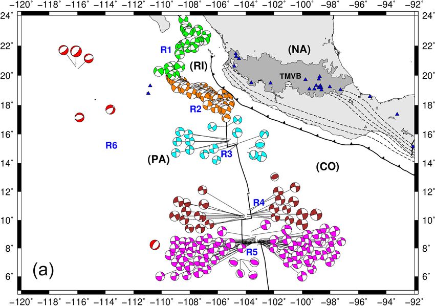
was divided into six sub-catalogues shown in Fig. 8 (R1 to was corroborated at a regional level by Rodríguez-Pérez and
R6). Zúñiga (2018). According to those authors, the highest b val-
ues correspond to normal-faulting events, followed by strike-
slip and thrust earthquakes, respectively. To characterize the
b value of oceanic earthquakes and compare the results with
other tectonic environments, we calculated the b value with a
robust method which has proven its validity in many stud-
ies. We estimated the b value by means of the maximum
www.solid-earth.net/11/791/2020/ Solid Earth, 11, 791–806, 2020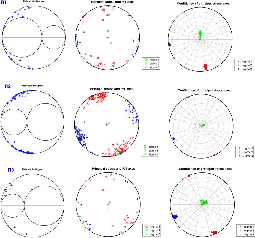
794                                          Q. Rodríguez-Pérez et al.: Seismicity characterization of oceanic earthquakes

likelihood formulation of Aki (1965) and the completeness         Tsallis entropy nonextensive framework (Tsallis, 1988). This
magnitude (Mc ) employing the maximum curvature method            model takes into consideration the irregular surfaces of two
(Wiemer and Wyss, 2000) with the aid of the ZMAP software         fault planes in contact and the rock fragments of different
package (Wiemer, 2001).                                           shape and sizes that fill the space between them. Accord-
   As reported by previous authors, seismicity on the             ing to this model, earthquakes are triggered by the interac-
mid-ocean transform faults is better represented by a ta-         tion along the fault planes of these rock fragments. Consid-
pered frequency-moment distribution (e.g., Boettcher and          ering that large fragments are more difficult to release than
McGuire, 2009). This distribution has the following form          small ones, the resulting energy is assumed to be propor-
(Kagan, 1997, 1999; Kagan and Jackson, 2000; Kagan and            tional to the volume of the fragment (Telesca, 2010). Silva
Schoenberg, 2001; Vere-Jones et al., 2001):                       et al. (2006) improved the model and found a scaling law
                                                                  between the released energy (ε) and the size of asperity frag-
             Mo β

                          Mo − M                                  ments (r) by the following proportional factor: ε ∝ r 3 . The
N (M) =No           exp             ,                 (1)
              M            Mm                                     nonextensive statistics are used to describe the volumetric
                                                                  distribution function of the fragments. A parameter that rep-
where β is one of the parameters to determine, β = (2/3)b,
                                                                  resents the proportion between ε and r is introduced. This
where b is the b value, N0 is the cumulative earthquake num-
                                                                  parameter is known as the a value or parameter a (Silva et
ber over a completeness threshold seismic moment (M0 ),
                                                                  al., 2006; Telesca, 2010). The parameter a is defined using
and Mm is the maximum expected moment. We analyzed
                                                                  a volumetric distribution function of the fragments applying
if this frequency distribution is suitable for describing the
                                                                  the maximum entropy principle for the Tsallis entropy (for
seismicity of oceanic events in Mexico. In order to cal-
                                                                  details in the mathematical expressions see Silva et al., 2006;
culate the tapered Gutenberg–Richter distribution, we used
                                                                  Telesca, 2010). The magnitude cumulative distribution func-
the MATLAB function Get_GR_parameters.m developed by
                                                                  tion becomes
Olive (2016). The tapered Gutenberg–Richter moment distri-
bution is fitted by mens of a least-squares inversion following                                     2−q
                                                                  log10 (N > M) = log10 (N) +                log10
Frohlich (2007).                                                                                    1−q
                                                                                  "                       !#
                                                                                                    10K

3.2.2     Temporal distribution of aftershocks                                            1−q
                                                                                    1−                        ,               (3)
                                                                                          2−q       a 2/3
The frequency distribution of the decrement of earthquake
aftershocks is described by the modified Omori’s law (Utsu,       where N is the total number of earthquakes; N (>M) repre-
1961; Utsu et al., 1995) as                                       sents the number of events with magnitude larger than M; a
                                                                  is a proportionality parameter between ε and r, and q is the
              k                                                   nonextensivity parameter. K is defined as K = 2M (Silva et
R (t) =            ,                                       (2)
          (t + c)p                                                al., 2006) or K = M (Telesca, 2011). The magnitude (M) is
where R(t) is the rate of occurrence of aftershocks within a      related to ε by the following relation: M = 1/3 log(ε) (Silva
given magnitude range, t is the time interval from the main-      et al., 2006). Telesca (2011) considered that the relation be-
shock, k is the productivity of the aftershock sequence, p is     tween ε and M is given by M = 2/3 log(ε). Neither of the
the power-law exponent (p value), and c is the time delay be-     two models is preferred over the other. We used both models
fore the onset of the power-law aftershock decay rate. Varia-     in order to quantify the variability in the nonextensive pa-
tions in p values exist for different tectonic regimes and each   rameters. According to Telesca (2010), the physical meaning
aftershock sequence. Many authors have related the p value        of the q parameter consists in that it provides information
with crustal temperature, heat-flow, or rock heterogeneity in     about the scale of interactions. It means that if q is close
the fault zone. Thus, relevant information can be extracted       to 1, the physical state is close to the equilibrium. As a re-
from these aftershock parameters in order to have a better        sult, few earthquakes are expected. On the other hand, as
understating of the rupture process of oceanic earthquakes.       q rises, the physical state goes away from the equilibrium
As before, we used the ZMAP software package (Wiemer,             state, this implies that the fault planes are able to generate
2001) for estimating the p value of the aftershock sequence       more earthquakes, thus resulting in an increment in the seis-
of the 1 May 1997 earthquake (Mw = 6.9).                          mic activity (Telesca, 2009, 2011). The physical meaning of
                                                                  the a value lies in the fact that it provides a measure of the
3.2.3     Fragment-asperity model                                 energy density. It means that the a value is large if the energy
                                                                  released is large (Telesca, 2011). For example, high a values
Alternative statistical models that relate the earthquake mag-    are expected when the events with the highest magnitude take
nitude distribution with the rheology of the fault have           place. Previous studies have shown that the q value ranges
been proposed. Among them, we have the fragment-asperity          mainly from 1.50 to 1.70 (Vilar et al., 2007; Vallianatos,
model. This model was introduced by Sotolongo-Costa and           2009; Rodríguez-Pérez and Zúñiga, 2017, among others). We
Posadas (2004) to describe the earthquake dynamics in a           obtained the a and q parameters by minimizing the root mean

Solid Earth, 11, 791–806, 2020                                                              www.solid-earth.net/11/791/2020/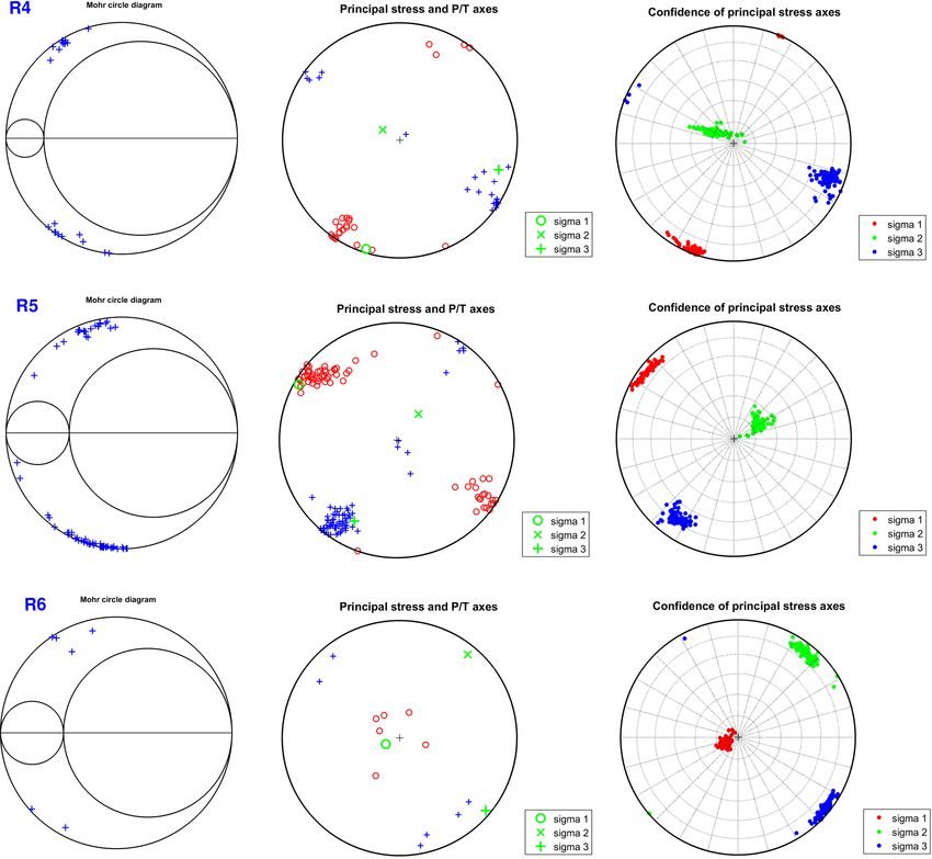
Q. Rodríguez-Pérez et al.: Seismicity characterization of oceanic earthquakes                                                       795

square error (RMS) with the Nelder–Mead method (Nelder
and Mead, 1965).

3.2.4   Stress inversion

Focal mechanisms are reliable indicators of the state of stress
in a tectonic region. In order to study the regional stress field
for oceanic earthquakes, we performed stress tensor inver-
sion from focal mechanisms reported in the Global CMT cat-
alogue (Dziewonski et al., 1981; Ekström et al., 2012) with
the iterative joint inversion developed by Vavryčuk (2014).
From the stress inversion, we obtained the orientation of the
principal stress axes σ1 , σ2 , and σ3 (where σ1 ≥ σ2 ≥ σ3 ) and
the stress ratio R. We now briefly explain each method. The
first method (the iterative joint inversion) provides an accu-
rate estimation of R and stress orientations (Vavryčuk, 2014).
In this method, the ratio is defined as R = (σ1 −σ2 )/(σ1 −σ3 )
(Gephart and Forsyth, 1984). A fault instability constraint
is applied, and the fault is identified with that nodal plane,      Figure 3. Main statistical characteristics for intraplate oceanic
which is more unstable and thus more susceptible to faulting        events (INT). (a) Magnitude earthquake histogram; (b) frequency–
(Vavryčuk, 2014). By incorporating a fault instability con-        magnitude distributions with Mc and b values. (c, d) The normal-
straint into the inversion, an iterative procedure is imposed.      ized cumulative number of events as function of magnitude for in-
The uncertainties are determined as the differences between         traplate oceanic events (INT). Color curves show the best fit for the
the inverted results considering noisy data (Vavryčuk, 2014).      nonextensivity parameters q and a for the Telesca (2010) (red lines)
The stress inversion was carried out with the STRESSIN-             and the Silva (2006) (green lines) models, respectively.
VERSE software developed by Vavryčuk (2014). The maxi-
mum horizontal stress (SHmax ) was calculated using the for-
mulation of Lund and Townend (2007). The stress inversion
was performed for each of the six different regions shown in        is in the range of 4.0–5.0 on average considering most of the
Fig. 7.                                                             global catalogues.
                                                                       Our results also showed that transform fault zone and mid-
                                                                    ocean ridge events follow a tapered Gutenberg–Richter dis-
4   Results                                                         tribution, as suggested in previous studies (Boettcher and
                                                                    McGuire, 2009). The tapered Gutenberg–Richter distribution
There is a large span of b values (Table 2) which nevertheless      was fitted with the following parameters: β = 0.64 and an
sheds light on the seismicity characteristics of oceanic earth-     estimated corner magnitude of Mm = 6.7 (Fig. 5a). These
quakes in Mexico. INT events exhibit higher b values and            results are in agreement with previous studies such as that
Mc than TF-MOR events (Figs. 3, 4a and Table 2). In par-            of Bird et al. (2002), which studied the tapered Gutenberg–
ticular, TF-MOR events also show local b-value variations in        Richter distribution for spreading ridges and oceanic trans-
the range of 0.72–1.30 (Fig. 4b) for each of the subregions         form faults based on global data, obtaining a β value of about
R1 to R5 (Table 2). Previous studies had shown large fluc-          0.67 for both types of events. They reported that Mm varies
tuations in b values of oceanic events. For example, Tolstoy        from 5.8 to 6.6–7.1 for mid-ocean ridge and transform faults,
et al. (2001) reported b values of about 1.5 associated with        respectively. The results for the nonextensive parameters are
volcanic activity in the Gakkel Ridge. Läderach (2011) re-          shown in Table 2. We found higher q values for TF-MOR
ported b values of 1.28 in the Southwest Indian Ridge. In a         events than for INT events (Fig. 5), meaning that TF-MOR
global study, Molchan et al. (1997) estimated the b value for       events are farther from the equilibrium than INT events. The
mid-ocean and transform zones, obtaining values of the fol-         results showed a better fit for cumulative distribution func-
lowing interval 0.97–1.47. In general, our b-value estimates        tions using the Telesca model for TF-MOR and each of the
agree with reported b values in previous studies. On the other      regions (Fig. 6). In regions R1-R5, our results showed that q
hand, our results showed that Mc for oceanic events is higher       varies from 1.31 to 1.52 and from 1.57 to 1.63 using Telesca’s
than reported Mc for the subduction zone and continental re-        and Silva’s models, respectively. In the case of subduction
gions of Mexico, which reflects the capability of the global        zones, the q value can vary from 1.35 to 1.70. For exam-
and regional networks to appropriately register events in that      ple, in the Hellenic Subduction Zone, q is in the range of
region. The magnitude completeness for oceanic earthquakes          1.35–1.55 (Papadakis et al., 2013); in the Mexican Subduc-
differs for different parts of the world, but in most cases, it     tion Zone, Valverde-Esparza et al. (2012) found that q varies

www.solid-earth.net/11/791/2020/                                                                    Solid Earth, 11, 791–806, 2020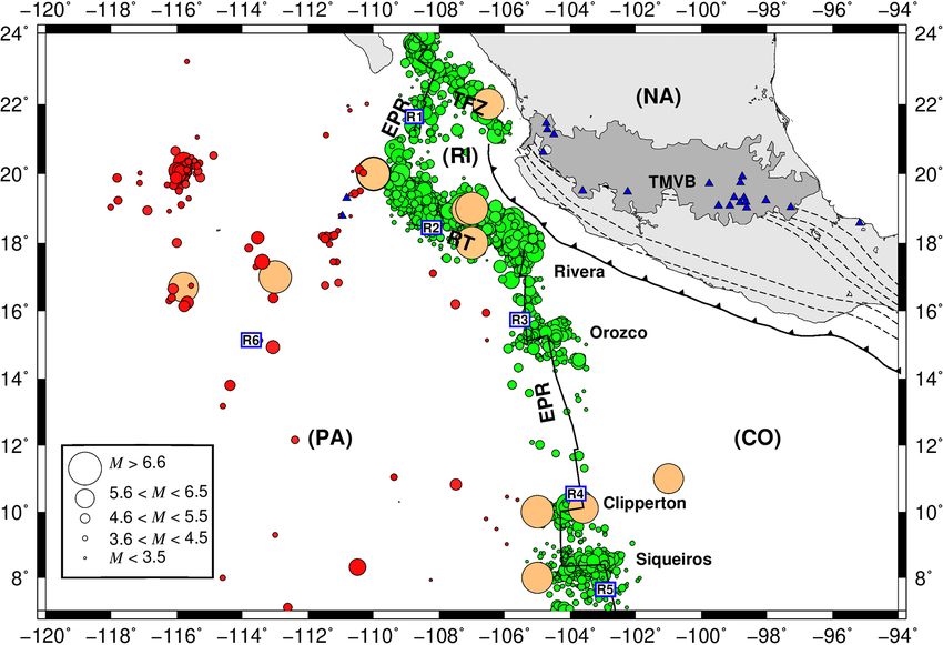
796                                                    Q. Rodríguez-Pérez et al.: Seismicity characterization of oceanic earthquakes

Figure 4. (a) Main statistical characteristics for the transform fault zone and mid-ocean ridge (TF-MOR) events (regions R1 to R5). (b) Mag-
nitude earthquake histograms and frequency–magnitude distributions with Mc and b values for each of the different subregions shown in
Fig. 8.

Table 2. Statistical parameters.

                          Type                        Mc      b value      qS value            aS value       qT value          aT value
                          INT                         4.4         0.89           1.60     6.69 × 10¹²              1.39      2.27 × 10⁶
                          TF-MOR (R1–R5)              4.1         0.64           1.60     3.22 × 10¹³              1.41      3.55 × 10⁶
                          R1                          4.1         0.72           1.62     3.22 × 10¹³              1.43      2.53 × 10⁶
                          R2                          4.0         0.77           1.62     1.24 × 10¹³              1.44      3.11 × 10⁶
                          R3                          4.4         1.30           1.57     6.81 × 10¹²              1.31      2.98 × 10⁶
                          R4                          4.4         0.75           1.70     1.12 × 10¹³              1.52      2.94 × 10⁶
                          R5                          4.3         0.94           1.63     5.79 × 10¹²              1.38      3.15 × 10⁶
                        INT are intraplate oceanic events; TF-MOR are transform fault zone and mid-ocean ridge events; Mc is the
                        completeness magnitude; b is the slope of the Gutenberg–Richter distribution; qS and aS and qT and aT are the
                        nonextensive parameters based on Silva et al. (2006) and Telesca (2011), respectively.

Solid Earth, 11, 791–806, 2020                                                                                            www.solid-earth.net/11/791/2020/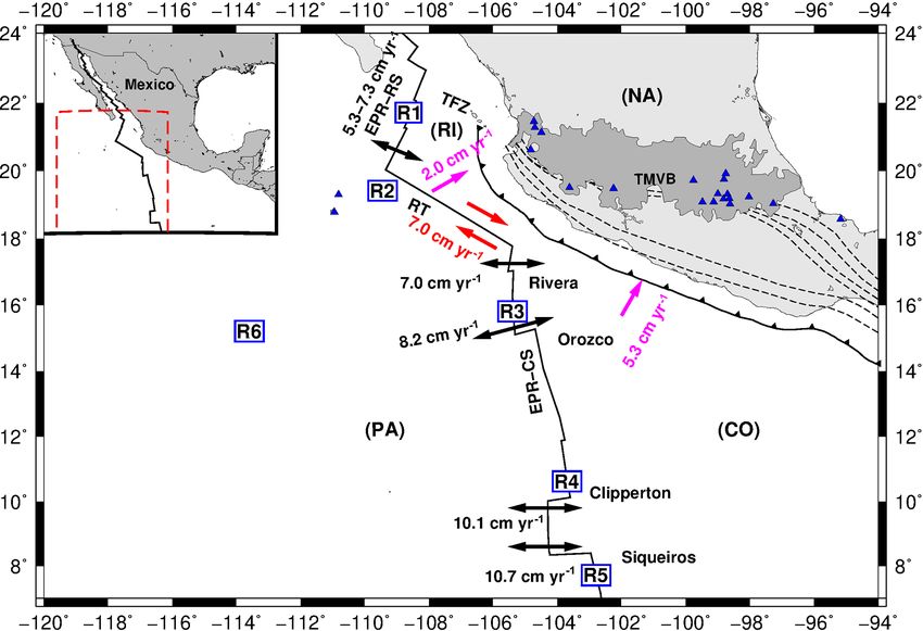
Q. Rodríguez-Pérez et al.: Seismicity characterization of oceanic earthquakes                                                          797

Figure 5. (a, b) The cumulative annual seismic moment frequency
distribution for the transform fault zone and mid-ocean ridge (TF-
MOR) events (regions R1 to R5). The blue lines are the moment,
tapered Gutenberg–Richter distributions. The red lines represent the
ordinary moment Gutenberg–Richter distributions. (c, d) The sub-
regions that do not follow an ordinary moment Gutenberg–Richter
distribution are subregions R1 and R2.
                                                                       Figure 6. The normalized cumulative number of events as func-
                                                                       tion of magnitude for the transform fault zone and mid-ocean ridge
from 1.63 to 1.70. Thus, our results conform to values ob-             (TF-MOR) events. Blue triangles show the completeness magnitude
tained in regional studies.                                            (Mc ). Red curves show the best fit for the nonextensivity parameters
   The analysis of the aftershock sequence of the 1 May 1997           q and a for Telesca’s (2010) model (red lines). Green curves show
earthquake (Mw = 6.9), yielded a p value of 0.67±0.33 (Ta-             the best fit for the nonextensivity parameters q and a for Silva’s
ble 3). The magnitude of the largest aftershock of the 1997            (2010) model (green lines).
event was Mw = 5.3 (Table 3). Oceanic strike-slip events
seem to have lower p values than mid-ocean ridge events. For
example, Bohnenstiehl et al. (2004) found a p value of 0.95            and (7) normal, N (Fig. 7). This classification was performed
for the 15 July 2003 (Mw = 7.6) central Indian Ridge strike-           to identify the dominant type of faulting for each subregion.
slip event. For the Siqueiros, Discovery, and western Blanco           Region R1 is composed of strike-slip (70.3 %), strike-slip
transforms, the p value varies from 0.94 to 1.29 (Bohnen-              with normal and reverse components (21.6 % and 5.4 %, re-
stiehl et al., 2002). Davis and Frohlich (1991) determined a           spectively), and normal-faulting (2.7 %) focal mechanisms
p value of 0.928 ± 0.024 for the combined ridge and trans-             (Fig. 7b). Region R2 exhibits the following focal mechanism
form environments. Our results fall within the range of global         distribution: strike-slip (82.4 %) and strike-slip with nor-
studies that showed that the p value varies from 0.6 to 2.5            mal and reverse components (9.5 % and 8.1 %, respectively)
(Utsu et al., 1995). We also reported a c close to 0 for the af-       (Fig. 7b). In region R3, the focal mechanism classification
tershock sequence of the 1 May 1997 (Mw = 6.9) (Table 3).              shows the following distribution: strike-slip (62.5 %), strike-
Shcherbakov et al. (2004) found that the parameter c of the            slip with normal component (25 %), normal-faulting with
Omori’s law decreases as the magnitude of events considered            strike-slip component (6.3 %), and reverse (6.3 %) (Fig. 7b).
increases. According to the study, this observation is due to          Region R3 consists of strike-slip (70.8 %), strike-slip with
the effect of an undercount of small aftershocks in short time         normal and reverse components (8.3 % and 16.7 %, respec-
periods. This provides an explanation for our result of c ∼ 0          tively), and reverse earthquakes (4.2 %) (Fig. 7b). Region R5
because of the limited magnitude detection reported in the             exhibits the following focal mechanism distribution: strike-
regional and global catalogues used.                                   slip (53 %), strike-slip with normal and reverse components
   We classified the focal mechanisms used in the stress in-           (23.5 % and 17.6 %, respectively), and reverse (5.9 %). For
version into seven categories: (1) reverse, R; (2) reverse with        the case of earthquakes in R6, the classification shows the
lateral component, R-SS; (3) strike-slip with reverse com-             following distribution: normal (83.3 %) and normal-faulting
ponent, SS-R; (4) strike-slip, SS; (5) strike-slip with normal         with strike-slip component (16.7 %) (Fig. 7b).
component, SS-N; (6) normal with lateral component, N-SS;

www.solid-earth.net/11/791/2020/                                                                       Solid Earth, 11, 791–806, 2020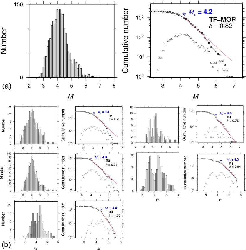
798                                                     Q. Rodríguez-Pérez et al.: Seismicity characterization of oceanic earthquakes

Table 3. Aftershocks characteristics of 1 May 1997 event.

                             Date (dd/mm/yyyy)             Mm       Ma        D            p value                    c                  k
                             01/05/1997                     6.9      5.3     1.6     0.67 ± 0.33         0.00 ± 0.53        2.12 ± 1.53
                           Mm is the magnitude of the mainshock; Ma is the magnitude of the largest aftershock; D is the difference in
                           magnitudes of the mainshock and its largest aftershock; p, c, and k are the coefficients of Omori’s law.

Table 4. Stress inversion results.

                        σ1 Azimuth/plunge            σ2 Azimuth/plunge             σ3 Azimuth/plunge            SHmax            R      Region
                        169◦ /16◦                                   2◦ /73◦                      260◦ /4◦          169◦      0.37            1∗
                        156◦ /0◦                                   62◦ /83◦                      246◦ /7◦          157◦      0.58            2∗
                        157◦ /4◦                                   31◦ /84◦                      247◦ /5◦          157◦      0.63            3∗
                        197◦ /3◦                                  302◦ /76◦                     106◦ /13◦           22◦      0.84            4∗
                        299◦ /6◦                                   44◦ /69◦                     207◦ /20◦          120◦      0.73            5∗
                        247◦ /80◦                                   39◦ /9◦                      130◦ /5◦           45◦      0.73            6∗
                      Stress ratio is defined by R = (σ1 − σ2 )/(σ1 − σ3 ); ∗ stress inversion based on Vavryčuk (2014) and Lund and
                      Townend (2007). Location of the regions are shown in Fig. 1.

   Table 4 summarizes the results from the stress inversion.
Based on the orientation of stress axes, a dynamical descrip-
tion of the tectonics of the oceanic earthquakes in Mexico can
be carried out. A quantitative comparison with other oceanic
regions is discussed in what follows. Region R6 is only dom-
inated by N and N-SS earthquakes (Fig. 8). In regions R4
and R5, stress results showed moderate similarities. The dif-
ferences in these regions may also be related to the variabil-
ity in focal mechanisms (here we have SS, SS-N, SS-R, and
to a lesser extent R events) (Fig. 8). Variations are very sig-
nificant in regions R1 to R3 (particularly in σ2 ) (Table 4).
These regions also showed different types of events: SS, SS-
N, and SS-R for R1; SS, SS-N, and SS-R for R2; and SS,
SS-N, N-SS, and R for R3 (Fig. 8). In these regions, strike-
slip earthquakes are the dominant type of faulting. Events
with unusual mechanisms have also been reported in other                                Figure 7.
oceanic regions. According to Wolfe et al. (1993), most of the
anomalous seismic activity is associated with mislocations,
complex fault geometry, or large structural features with an
influence on the slip of the fault. DeMets and Stein (1990)                             is in the NE–SW direction for the T axis. In region R3, σ2
showed that the strike direction and earthquake slip vectors                            is almost vertical, and the SHmax is also 157◦ , suggesting
in the Rivera Transform are rotated clockwise from the ex-                              a strike-slip regime. The orientation of the P axis is in the
pected direction of the Pacific–Rivera Euler vector. This de-                           NW–SE direction. The main orientation of the T axes is NE–
viation can be the result of morphologic features resulting in                          SW, but E–W directions occur as well. For the region R4, σ2
unusual patterns of epicenters and focal mechanisms.                                    is 76, and the SHmax is 22◦ , suggesting a strike-slip regime.
   In the case of the East Pacific Rise Rivera segment (re-                             The predominant orientations of the P and T axes are NE–
gion R1), σ2 is almost vertical, and SHmax is ∼ 170◦ , sug-                             SW and NW–SE, respectively. In R5, σ2 is from 69◦ , and
gesting a strike-slip regime (Table 4). The main orientations                           the SHmax is 120◦ , suggesting a strike-slip regime. The main
of the P axes are in the N–S, NW–SE, and E–W directions.                                orientation of the P axes is NW–SE, while that of the T axis
The orientations of the P axes are NW–SE and, to a lesser                               is NE–SW. In R6, the principal axes are related to a normal
extent, E–W directions (Fig. 9). For the case of the Rivera                             fault regime. σ1 is almost vertical, and the SHmax is ∼ 45◦ .
Transform (region R2), σ2 is quasi vertical, and the SHmax                              The orientation of the T axes is in the NW–SE direction.
is 157◦ , suggesting a strike-slip regime. The orientation of                           The Mohr circle diagram showed that most of the studied
the P axes is in the NW–SE direction, and the orientation                               events are clustered along the outer Mohr’s circle in the area
                                                                                        of validity of the Mohr–Coulomb failure criterion (Fig. 9).

Solid Earth, 11, 791–806, 2020                                                                                              www.solid-earth.net/11/791/2020/
Q. Rodríguez-Pérez et al.: Seismicity characterization of oceanic earthquakes 799
Figure 7. Focal mechanism solutions of oceanic earthquakes in
Mexico reported by the Global CMT catalogue from 1976 to 2017.
(a) Focal mechanisms are divided into six regions (R1 to R6) for the
stress inversion analysis. (b) Focal mechanism classification based
on the Kaverina et al. (1996) projection technique implemented
by Álvarez-Gómez (2015): reverse, reverse with lateral component,
strike-slip with reverse component, strike-slip, strike-slip with nor-
mal component, normal with lateral component, and normal (R, R-
SS, SS-R, SS, SS-N, N-SS, and N, respectively).
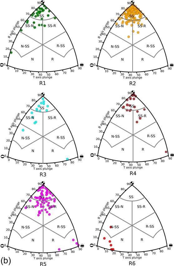
Figure 8. Orientation of horizontal axes. (a) Maximum horizontal
stresses (SH); (b) Minimum horizontal stresses (Sh).
Reported focal mechanisms confirm Sykes’s model for mid-
ocean ridges (Sykes, 1967), where events in transform zones
tend to have strike-slip mechanisms, while ridge crest events
have mainly normal faults. The obtained orientation of the first discuss the magnitude completeness of oceanic earth-
principal axes supports this model. quakes. Global studies showed that the magnitude complete-
ness for oceanic earthquakes is in the range of 4.0–5.0. Our
results are in agreement with these global studies. However,
5 Discussion as expected, several microseismic surveys which have been
conducted in different oceanic environments (e.g., Smith et
One of the main problems for studying oceanic seismicity is al., 2003; Simão et al., 2010; McGuire et al., 2012, among
that the epicenters are located far from most of the record- others) can yield lower-magnitude thresholds. As a result of
ing stations in mainland Mexico. This has a direct effect on these studies, precise hypocenter locations and earthquake
the earthquake magnitude distributions (Mc and b value). We distributions with a broader magnitude range were obtained.
www.solid-earth.net/11/791/2020/ Solid Earth, 11, 791–806, 2020800 Q. Rodríguez-Pérez et al.: Seismicity characterization of oceanic earthquakes Thus, lower Mc has been reported for studies based on mi- occurrence, duration, and magnitude. Earthquake statisti- croseismic surveys. For example, in the Mid-Atlantic Ridge, cal studies showed that large oceanic events in transform Mc ∼ 3.0 with several smaller events (Mw 6.5 in the Rivera Transform. According to McGuire et vious studies, extremely high p values (p>2) and short af- al. (2012), the apparent lack of large events on mid-ocean tershock durations are related to high temperatures (Bohnen- ridge transform faults may also be related to the heterogene- stiehl et al., 2002; Simão et al., 2010) and/or migration of hy- ity of materials on the fault plane. The maximum magnitude drothermal fluids (Goslin et al., 2005). We found a p value of for transform fault events on the East Pacific Rise (in the lat- 0.67 ± 0.33 for the 1 May 1997 (Mw = 6.9) strike-slip event itude interval of 3◦ < Lat < 5◦ ) is about 6.5 (McGuire et al., in the Rivera Transform. This p value is consistent with other 2005). On the other hand, earthquakes in the Rivera Trans- oceanic regions, but it does not seem to conform to a high- form and on the northern segment of the East Pacific Rise temperature regime. (in Mexico) have relative larger magnitudes (M>6.8) based Regarding the magnitude distribution of oceanic events, on reported seismicity in different catalogues (Fig. 1). This our b-value estimates are in agreement with global highlights a differentiation between the middle and southern oceanic studies but differ from local studies. For exam- and northern segments of the East Pacific Rise. ple, along the East Pacific Rise (in the latitude interval A further aspect of the analysis of oceanic earthquakes is of 5◦ N < Lat < 9.90◦ N), b-value estimations fluctuate from their capacity to generate aftershocks as well as the their 1.10 to 2.50 (Bohnenstiehl et al., 2008). Bohnenstiehl et Solid Earth, 11, 791–806, 2020 www.solid-earth.net/11/791/2020/
Q. Rodríguez-Pérez et al.: Seismicity characterization of oceanic earthquakes                                                801

Figure 9.

al. (2008) determined the b value of 9000 microearthquakes       heterogeneity, fewer magnitude events would be expected
with magnitudes in the range of −1.5–1.0 located in the          (reducing the b value). Another explanation for the differ-
southern part of our study zone. Due to this overlap, we com-    ences between our results and the results of Bohnenstiehl
pare their results with our results for region R5. For this      et al. (2008) is that the magnitude ranges of the earthquake
region, we obtained a b value of 0.94 with a Mc of 4.2,          catalogues are extremely different. This highlights how the
while they found that the b value approaches 2.5 at very         b value is affected by magnitude completeness.
shallow depths (< 0.3 km) (with Mc = −1.3). At depths of            Statistical studies suggested that the β value mainly takes
0.5–1.5 km, the b values drop to a value of 1.10 (with Mc =      values between 0.60 and 0.70 for a global range (Kagan,
−0.4). According to Bohnenstiehl et al. (2008) at very shal-     2002). Our estimates of β agree with global oceanic stud-
low depths, the uppermost oceanic crust is structurally het-     ies. It is essential to discuss the tectonic implications of this
erogeneous because of the extrusion of lava and the repeated     parameter. Bird et al. (2002) also found a dependence of
emplacement of sheeted dikes. As a consequence, there is a       β value on the relative plate velocity. According to them,
large proportion of small versus large earthquakes resulting     the β value is higher (with Mm = 7.1) when the velocity is
in high b values. The b values decrease with depth due to the    < 36 mm yr−1 than when the velocity is > 67 mm yr−1 (with
decreasing heterogeneity and/or changes in ambient stress        Mm = 6.6) for spreading ridges and oceanic transform faults,
levels. Considering that events in our catalogue for R5 oc-      respectively. These observations are in agreement with our
cur at a different depth interval, and assuming the decreasing   estimate of β = 0.64 and Mm of 6.6 for oceanic earthquakes

www.solid-earth.net/11/791/2020/                                                               Solid Earth, 11, 791–806, 2020
802                                             Q. Rodríguez-Pérez et al.: Seismicity characterization of oceanic earthquakes

Figure 9. Mohr circle diagrams for all the regions (left column). P and T axes distributions for all the regions (right column). Red circles
represent pressure, while blue crosses represent tension.

in Mexico (Fig. 5). For intraplate events, we obtained a                models (Fig. 5). Both models showed that a for TF-MOR is
β>0.70. According to Kagan (2010), β values > 0.70 may                  higher than a for the INT events (Fig. 5). This implies that
be related to the mix of earthquake populations with different          more energy is released for TF-MOR earthquakes. On the
maximum magnitudes (Mm ). In the case of intraplate events,             other hand, the q value indicates if the physical state of a seis-
we associated the somewhat high β values with the mix of                mic area moves away from equilibrium. The physical state is
some intraplate and mid-ocean–transform events. This could              at equilibrium when q is equal to 1, and as q increases, the
be related to incorrect hypocenter locations due to the diffi-          system is in an instability state in which a more significant
culty of precisely locating oceanic events by the land-based            amount of seismic energy is released.
networks.                                                                  Finally, we discuss the focal mechanisms and the calcu-
   The seismicity models based on nonextensivity consider               lated state of stress for oceanic earthquakes in Mexico. Focal
the interaction of two irregular fault surfaces (asperities) and        mechanisms provide useful information about the structure
rock fragments filling them. However, these models differ in            and settings of faults and can describe the crustal stress field
their assumption of how energy is stored in the fragments               in which earthquakes take place. Our analysis is limited be-
and the asperities. This difference is expressed through the            cause we only used focal mechanisms based on teleseismic
constant a, which represents the proportionality between the            data. The teleseismic detection threshold for oceanic events
released energy E and the fragment size r. This explains                in the East Pacific Rise is dependent on the region of the
the difference in a parameter between Telesca’s and Silva’s             EPR. For example, Riedesel et al. (1982) report a magnitude

Solid Earth, 11, 791–806, 2020                                                                      www.solid-earth.net/11/791/2020/
Q. Rodríguez-Pérez et al.: Seismicity characterization of oceanic earthquakes                                                     803

detection threshold in the range of 4.0–5.0. For the Quebrada,     rate of the 1 May 1997 (Mw = 6.9) strike-slip event in the
Discovery, and Gofar faults, the CMT catalogue is only com-        Rivera Transform is also consistent with oceanic p-value es-
plete to MW = 5.4. (McGuire, 2008; Wolfson-Schwehr et al.,         timations. Despite the limitation of the catalogues used, our
2014). Another limitation of our study is that we combine          results provided a comprehensive insight into the seismic-
different types of earthquakes into a single region, resulting     ity of oceanic environments. The main problem is the lo-
in inaccurate estimations of the stress state for that specific    cation uncertainty and mislabeling of the earthquakes. The
region. Under these circumstances, our study provides infor-       b value for INT events (1.17) is higher than that for TF-
mation on the stress field of major structures or the stress       MOR events (0.82). Our b-value estimations are in agree-
associated with the dominant types of earthquakes.                 ment with other regional studies but differ from b-value es-
   In oceanic environments, the largest magnitude events           timates based on microseismicity studies. Our b-value esti-
along transform fault or intraplate earthquakes usually show       mates for mid-ocean ridge/transform fault environments are
strike-slip mechanisms (Wiens and Stein, 1984; Kawasaki et         lower (0.72
804                                               Q. Rodríguez-Pérez et al.: Seismicity characterization of oceanic earthquakes

Competing interests. The authors declare that they have no conflict        S. and Freymueller, J. T., American Geophysical Union, 203–
of interest.                                                               218, 2002.
                                                                         Boettcher, M. S. and Jordan, T. H.: Seismic behavior of oceanic
                                                                           transform faults, Fall Meeting, American Geophysical Union
Acknowledgements. We thank the Mexican National Seismologi-                (AGU), San Francisco, California, 10–14 December, 1–2, 2001.
cal Service (SSN) for providing us with the earthquake catalogue.        Boettcher, M. S. and Jordan, T. H.: Earthquake scaling relations for
Station maintenance, data acquisition, and distribution are thanks         mid-ocean ridge transform faults, J. Geophys. Res., 109, B12302,
to its personnel. Quetzalcoatl Rodríguez-Pérez was supported by            https://doi.org/10.1029/2004JB003110, 2004.
the Mexican National Council for Science and Technology (CONA-           Boettcher, M. S. and McGuire, J. J.: Scaling relations for seismic
CYT) (Catedras program, project 1126).                                     cycles on mid-ocean ridge transform faults, Geophys. Res. Lett.,
                                                                           36, L21301, https://doi.org/10.1029/2009GL040115, 2009.
                                                                         Boettcher, M. S., Hirth, G., and Evans, B.: Olivine friction at
Financial support. This research has been supported by the                 the base of oceanic seismogenic zones, J. Geophys. Res., 112,
CONACYT (grant no. Catedras program, project 1126).                        B01205, https://doi.org/10.1029/2006JB004301, 2007.
                                                                         Boettcher, M. S., Wolfson-Schwehr, M. L., Forestall, M., and Jor-
                                                                           dan, T. H.: Characteristics of oceanic strike-slip earthquakes dif-
                                                                           fer between plate boundary and intraplate settings, Fall Meeting,
Review statement. This paper was edited by Irene Bianchi and re-
                                                                           American Geophysical Union (AGU), San Francisco, California,
viewed by two anonymous referees.
                                                                           3–7 December, Seismology, 2012, 7245, 2012.
                                                                         Bohnenstiehl, D. R., Tolstoy, M., Dziak, R. P., Fox, C. G., and
                                                                           Smith, D. K.: Aftershock sequences in the mid-ocean ridge envi-
References                                                                 ronment: an analysis using hydroacoustic data, Tectonophysics,
                                                                           354, 49–70, 2002.
Abe, K.: Magnitudes of large shallow earthquakes from 1904 to            Bohnenstiehl, D. R., Tolstoy, M., and Chapp, E.: Breaking into
  1980, Phys. Earth Planet. Int., 27, 72–92, 1981.                         the plate: A 7.6 Mw fracture-zone earthquake adjacent to
Abercrombie, R. E. and Ekström, G.: Earthquake slip on oceanic             the central Indian Ridge, Geophys. Res. Lett., 31, L02615,
  transform faults, Nature, 410, 74–77, 2001.                              https://doi.org/10.1029/2003GL018981, 2004.
Abercrombie, R. E. and Ekström, G.: A reassessment of the rup-           Bohnenstiehl, D. R., Waldhauser, F., and Tolstoy, M.: Frequency-
  ture characteristics of oceanic transform earthquakes, J. Geo-           magnitude distribution of microearthquakes beneath the
  phys. Res., 108, 1–9, 2003.                                              9◦ 50’N region of the East Pacific Rise, October 2003
Aki, K.: Maximum likelihood estimate of b in the formula log(N) =          through April 2004, Geochem. Geophy. Geosy., 9, Q10T03,
  a − bM and its confidence limits, B. Earthq. Res. I. Tokyo, 43,          https://doi.org/10.1029/2008GC002128, 2008.
  237–239, 1965.                                                         Choy, G. L. and Boatwright, J.: Global patterns of radiated seismic
Álvarez-Gómez, J. A.: FMC: A program to manage, classify and               energy and apparent stress, J. Geophys. Res., 100, 18205–18226,
  plot focal mechanism data, Version 1.01, 1–27, 2015.                     1995.
Antolik, M., Abercrombie, R., Pan J., and Ekström, G:                    Choy, G. L. and McGarr, A.: Strike-slip earthquakes in the oceanic
  Rupture characteristics of the 2003 Mw 7.6 mid-Indian                    lithosphere: Observations of exceptionally high apparent stress,
  Ocean earthquake: implications for seismic properties of                 Geophys. J. Int., 100, 18205–18226, 2002.
  young oceanic lithosphere, J. Geophys. Res., 111, B04302,              Cowie, P. A., Scholz, C. H., Edwards, M., and Malinverno, A.: Fault
  https://doi.org/10.1029/2005JB003785, 2006.                              strain and seismic coupling on Mid-Ocean Ridges, J. Geophys.
Bandy, W. L.: Geological and geophysical investigation of the              Res., 98, 17911–17920, 1993.
  Rivera-Cocos plate boundary: implications for plate fragmenta-         Davis, S. D. and Frohlich, C.: Single-link cluster analysis, synthetic
  tion, Ph.D. thesis, Texas A&M University, College Station, 195           earthquake catalogues and aftershock identification, Geophys. J.
  pp., 1992.                                                               Int., 104, 289–306, 1991.
Bandy, W. L., Michaud, F., Mortera Gutierrez, C. A., Dyment, J.,         DeMets , C., Gordon, R. G., Argus, D. F., and Stein, S.: Effect of re-
  Bourgois, J., Royer, J. Y., Calmus, T., Sosson, M., and Ortega-          cent revisions to the geomagnetic reversal time scale on estimate
  Ramirez, J.: The Mid-Rivera-Transform discordance: morphol-              of current plate motions, Geophys. Res. Lett., 21, 2191–2194,
  ogy and tectonic development, Pure Appl. Geophys., 168, 1391–            1994.
  1413, 2011.                                                            Dziewonski, A. M., Chou, T. A., and Woodhouse, J. H.: Determi-
Bergman, E. A.: Intraplate earthquakes and the state of stress in          nation of earthquake source parameters from waveform data for
  oceanic lithosphere, Tectonophysics, 132, 1–35, 1986.                    studies of global and regional seismicity, J. Geophys. Res., 86,
Bergman, E. A. and Solomon, S. C.: Oceanic intraplate earthquakes:         2825–2852, 1981.
  implications for local and regional intraplate stress, J. Geophys.     Ekström, G., Nettles, M., and Dziewonski, A. M.: The global CMT
  Res., 85, 5389–5410, 1980.                                               project 2004-2010: centroid-moment tensors for 13,017 earth-
Beroza, G. C. and Jordan, T.: Searching for slow and silent earth-         quakes, Phys. Earth Planet. Int., 200/201, 1–9, 2012.
  quakes using free oscillations, J. Geophys. Res., 95, 2485–2510,       Frohlich, C.: Practical suggestions for assessing rates of seismic-
  1990.                                                                    moment release, B. Seismol. Soc. Am., 97, 1158–1166, 2007.
Bird, P., Kagan, Y. Y., and Jackson, D. D.: Plate tectonics and earth-   Gephart, J. W. and Forsyth, D. W.: An improved method for deter-
  quake potential of spreading ridges and oceanic transform faults,        mining the regional stress tensor using earthquake focal mecha-
  in: Plate Boundary Zones, Geodynamics Series, edited by: Stein,

Solid Earth, 11, 791–806, 2020                                                                        www.solid-earth.net/11/791/2020/
Q. Rodríguez-Pérez et al.: Seismicity characterization of oceanic earthquakes 805 nism data: application to the San Fernando earthquake sequence, Lund, B. and Townend, J.: Calculating horizontal stress orientations J. Geophys. Res., 89, 9305–9320, 1984. with full or partial knowledge of the tectonic stress tensor, Geo- Goslin, J., Benoit, M., Blanchard, D., Bohn, M., Dosso, L., Dreher, phys. J. Int., 270, 1328–1335, 2007. S., Etoubleau, J., Gente, P., Gloaguen, R., Imazu, Y., Luis, J., McGuire, J. J.: Seismic cycles and earthquake predictability on East Maia, M., Merkouriev,S., Oldra, J.-P., Patriat, P., Ravilly, M., Pacific Rise transform faults, B. Seismol. Soc. Am., 98, 1067– Souriot, T., Thirot, J.-L., and Yama-ashi, T.: Extent of Azores 1084, 2008. plume influence on the Mid-Atlantic Ridge north of the hotspot, McGuire, J. J., Ihmlé, P. F., and Jordan, T. H.: Time-domain ob- Geology, 27, 991–994, 1999. servations of a slow precursor to the 1994 Romanche transform Goslin, J., Lourenço, N., Dziak, R.P., Bohnenstiehl, D. R., Haxel, J., earthquake, Science, 274, 82–85, 1996. and Luis, J.: Long-term seismicity of the Reykjanes Ridge (North McGuire, J. J., Boettcher M. S., and Jordan, T. H.: Foreshock se- Atlantic) recorded by a regional hydrophone array, Geophys. J. quences and short-term earthquake predictability on East Pacific Int., 162, 516–524, 2005. Rise transform faults, Nature, 434, 457–461, 2005. Gutenberg, B. and Richter, C. F.: Frequency of earthquakes in Cali- McGuire, J. J., Collins, J. A., Gouédard, P., Roland, E., and fornia, B. Seismol. Soc. Am., 34, 185–188, 1944. Lizarralde, D.: Variations in earthquake rupture properties along Houston, H., Anderson, H., Beck., S. L., Zhang, J., and Schwartz, the Gofar transform fault, East Pacific Rise, Nat. Geosci., 5, 336– S.: The 1986 Kermadec earthquake and its relation to plate seg- 341, 2012. mentation, Pure Appl. Geophys., 140, 331–364, 1993. Mogi, K.: Magnitude-frequency relation for elastic shocks accom- Hwang, L. J. and Kanamori, H.: Rupture process of the 1987– panying fractures of various materials and some related problems 1988 Gulf of Alaska earthquake sequence, J. Geophys. Res., 97, in earthquakes, B. Earthq. Res. I. Tokyo, 40, 831–853, 1962. 19881–19908, 1992. Molchan, G., Kronrod, T., and Panza, G. F.: Multi-scale seismicity Ihmlé, P. F. and Jordan, T. H.: Teleseismic search for slow precur- model for seismic risk, B. Seismol. Soc. Am., 87, 1220–1229, sors to large earthquakes, Science, 266, 1547–1551, 1994. 1997. International Seismological Centre: On-line Bulletin and catalog, Nelder, J. A. and Mead, R.: A simplex method for function mini- https://doi.org/10.31905/D808B830, 2020. mization, Comput. J., 7, 308–313, 1965. Ishimoto, M. and Iida, K.: Observations of earthquakes registered Nuannin, P., Kulhanek, O., and Persson, L.: Variations of b-value with the microseismograph constructed recently, B. Earthq. Res. preceding large earthquakes in the Andaman-Sumatra subduc- I. Tokyo, 17, 443–478, 1939. tion zone, J. Asian Earth Sci., 61, 237–242, 2012. Kagan, Y. Y.: Seismic moment-frequency relation for shallow earth- Okal, E. A. and Stewart, L. M.: Slow earthquakes along oceanic quakes: regional comparisons, J. Geophys. Res., 102, 2835– fracture zones: evidence for asthenospheric flow away from 2852, 1997. hotspots?, Earth Planet. Sc. Lett., 57, 75–87, 1992. Kagan, Y. Y.: Universality of the seismic moment-frequency rela- Olive, J.-A.: Get_GR_parameters.m Matlab function for analysis tion, Pure Appl. Geophys., 155, 537–573, 1999. of earthquake catalogs, available at: https://jaolive.weebly.com/ Kagan, Y. Y.: Seismic moment distribution revisited: I. Statistical codes.html (last acces: 23 December 2019), 2016. results, Geophys. J. Int., 148, 520–541, 2002. Pacheco, J. F. and Sykes, L. R.: Seismic moment catalog of large Kagan, Y. Y.: Earthquake size distribution: power-law with expo- shallow earthquakes, 1900 to 1989, B. Seismol. Soc. Am., 82, nent β ≡ 1/2?, Tectonophysics, 490, 103–114, 2010. 1306–1349, 1992. Kagan, Y. Y. and Jackson, D. D.: Probabilistic forecasting of earth- Papadakis, G., Vallianatos, F., and Sammonds, P.: Evidence of quakes, Geophys. J. Int., 143, 438–453, 2000. nonextensive statistical physics behavior of the Hellenic subduc- Kagan, Y. Y. and Schoenberg, F.: Estimation of the upper cutoff tion zone seismicity, Tectonophysics, 608, 1037–1048, 2013. parameter for the tapered pareto distribution, J. Appl. Probab. A, Pockalny, R. A., Fox, P. J., Fornari, D. J., McDonald, K., and 38, 158–175, 2001. Perfit, M. R.: Tectonic reconstruction of the Clipperton and Kanamori, H. and Stewart, G. S.: Mode of the strain release along Siqueiros Fracture zones: evidence and consequences of plate the Gibbs fracture zone, Mid-Atlantic Ridge, Phys. Earth Planet. motion change for the last 3 Myr, J. Geophys. Res., 102, 3167– Int., 11, 312–332, 1976. 3181, 1997. Kaverina, A. N., Lander, A. V., and Prozorov, A. G.: Global creepex Rabinowitz, N. and Steinberg, D. M.: Aftershock decay of the three distribution and its relation to earthquake-source geometry and recent strong earthquakes in the Levant, B. Seismol. Soc. Am., tectonic origin, Geophys. J. Int., 125, 249–265, 1996. 88, 1580–1587, 1998. Kawasaki, I., Kawahara, Y., Takata, I., and Kosugi, I.: Mode of seis- Riedesel, M., Orcutt, J. A., McDonald, K. C., and McClain, J. S.: mic moment release at transform faults, Tectonophysics, 118, Microearthquakes in the Black Smoker Hydrothermal Field, east 313–327, 1985. Pacific Rise at 21◦ N, J. Geophys. Res., 87, 10613–10623, 1982. Kisslinger, C.: Aftershocks and fault-zone properties, Adv. Geo- Rodríguez-Pérez, Q. and Zúñiga, F. R.: Seismicity characterization phys., 38, 1–36, 1996. of the Maravatío-Acambay and Actopan regions, central Mexico, Klein, F. W., Wright, T., and Nakata, J.: Aftershock decay, pro- J. S. Am. Earth Sci., 76, 264–275, 2017. ductivity, and stress rates in Hawaii: indicators of temperature Rodríguez-Pérez, Q. and Zúñiga, F. R.: Imaging b-value depth vari- and stress from magma sources, J. Geophys. Res., 111, B07307, ations within the Cocos and Rivera plates at the Mexican subduc- https://doi.org/10.1029/2005JB003949, 2006. tion zone, Tectonophysics, 734, 33–43, 2018. Läderach, C.: Seismicity of ultraslow spreading mid-ocean ridges at Roland, E., Behn, M. D., and Hirth, G.: Thermal-mechanical behav- local, regional and teleseismic scales: A case study of contrasting ior of oceanic transform faults: Implications for the spatial dis- segments, Ph.D thesis, University of Bremen, 116 pp., 2011. www.solid-earth.net/11/791/2020/ Solid Earth, 11, 791–806, 2020
806                                               Q. Rodríguez-Pérez et al.: Seismicity characterization of oceanic earthquakes

   tribution of seismicity, Geochem. Geophy. Geosy., 11, Q07001,         Utsu, T.: Statistical features of seismicity, International Handbook
   https://doi.org/10.1029/2010GC003034, 2010.                              of Earthquake and Engineering Seismology, Part A, Academic
Scholz, C. H.: The frequency-magnitude relation of micro fractur-           Press, 719–732, 2002.
   ing in rock and its relation to earthquakes, B. Seismol. Soc. Am.,    Utsu, T., Ogata, Y., and Matsura, R. S.: The centenary of the Omori
   58, 388–415, 1968.                                                       formula for a decay law of aftershock activity, J. Phys. Earth., 43,
Schorlemmer, D. S., Wiemer, S., and Wyss, M.: Variations in                 1–33, 1995.
   earthquake-size distribution across different stress regimes, Na-     Vallianatos, F.: A non-extensive approach to risk assessment, Nat.
   ture, 437, 539–542, 2005.                                                Hazards Earth Syst. Sci., 9, 211–216, 2009.
Scordilis, E. M.: Empirical global converting Ms and mb to moment        Valverde-Esparza, S. M., Ramirez-Rojas, A., Flores-Marquez, E.
   magnitude, J. Seismol., 10, 225–236, 2006.                               L., and Telesca, L.: Non-extensivity analysis of seismicity within
Servicio       Sismológico        Nacional:       On-line     catalog,      four subduction regions in Mexico, Acta Geophys., 60, 833–845,
   https://doi.org/10.21766/SSNMX/SN/MX, 2020.                              2012.
Shcherbakov, R., Turcotte, D. L., and Rundle, J. B.: A generalized       Vavryčuk, V.: Iterative joint inversion for stress and fault orienta-
   Omoris’s law for earthquakes aftershocks decay, Geophys. Res.            tions from focal mechanisms, Geophys. J. Int., 199, 69–77, 2014.
   Lett., 31, L11613, https://doi.org/10.1029/2004GL019808, 2004.        Velasco, A. A., Ammon, C. J., and Beck, S. L.: Broadband source
Silva, R., Franca, G., Vilar, C., and Alcaniz, J.: Nonexten-                modeling of the November 8, 1997, Tibet (Mw = 7.5) earthquake
   sive models for earthquakes, Phys. Rev. E, 73, 026102,                   and its tectonic implications, J. Geophys. Res., 105, 28065–
   https://doi.org/10.1103/PhysRevE.73.026102, 2006.                        28080, 2000.
Simão, N., Escartín, J., Goslin, J., Haxel, J., Cannat, M., and Dziak,   Vere-Jones, D., Robinson, R., and Yang, W. Z.: Remarks on the
   R.: Regional seismicity of the Mid-Atlantic Ridge: observa-              accelerated moment release model: problems of model formula-
   tions from autonomous hydrophone arrays, Geophys. J. Int., 183,          tion, simulation and estimation, Geophys. J. Int., 144, 517–531,
   1559–1578, 2010.                                                         2001.
Smith, D. K., Tolstoy, M., Fox, C. G., Bohnenstiehl, D. R., Mat-         Vilar, C. S., Franca, G., Silva, R., and Alcaniz, J. S.: Nonextensivity
   sumoto, H., and Fowler, M. J.: Hydroacoustic monitoring of seis-         in geological faults?, Physica A, 377, 285–290, 2007.
   micity at the slow-spreading Mid-Atlantic Ridge, Geophys. Res.        Warren, N. W. and Latham, G. V.: An experimental study of the
   Lett., 29, 13-1–13-4, 2002.                                              thermally induced microfracturing and its relation to volcanic
Smith, D. K., Escartin, J., Cannat, M., Tolstoy, M., Fox,                   seismicity, J. Geophys. Res., 75, 4455–4464, 1970.
   C. G., Bohnenstiehl, D. R., and Bazin, S.: Spatial and                Wesnousky, S. G.: The Gutenberg-Richter or characteristic earth-
   temporal distribution of seismicity along the northern                   quake distribution, which is it?, B. Seismol. Soc. Am., 84, 1940–
   Mid-Atlantic Ridge (15◦ –35◦ ), J. Geophys. Res., 108,                   1959, 1994.
   https://doi.org/10.1029/2002JB001964, 2003.                           Wiemer, S.: A software package to analyze seismicity: ZMAP, Seis-
Smith, W. D.: The b-value as an earthquake precursor, Nature, 289,          mol. Res. Lett., 72, 373–382, 2001.
   136–139, 1981.                                                        Wiemer, S. and Benoit, J. P.: Mapping the b-value anomaly at
Sotolongo-Costa, O. and Posadas, M. A.: Fragment-asperity in-               100 km depth in the Alaska and New Zealand subduction zones,
   teraction model for earthquakes, Phys. Rev. Lett., 92, 048501,           Geophys. Res. Lett., 23, 1557–1560, 1996.
   https://doi.org/10.1103/PhysRevLett.92.048501, 2004.                  Wiemer, S. and Wyss, M.: Minimum magnitude of completeness
Stein, S. and Pelayo, A.: Seismological constraints on stress in the        in earthquake catalogues: Examples from Alaska, the western
   oceanic lithosphere, Philos. T. R. Soc. Lond., 337, 53–72, 1991.         United States, and Japan, B. Seismol. Soc. Am., 90, 859–869,
Sykes, L. R.: Mechanism of earthquakes and nature of faulting on            2000.
   the mid-oceanic ridges, J. Geophys. Res., 72, 2131–2153, 1967.        Wiemer, S. and Wyss, M.: Mapping spatial variability of the
Telesca, L.: Nonextensive analysis of seismic sequences, Physica A,         frequency-magnitude distribution of earthquakes, in: Advances
   389, 1911–1914, 2009.                                                    in geophysics, Vol. 45, 259 pp., Elsevier, 2002.
Telesca, L.: A non-extensive approach in investigating the seismic-      Wiens, D. A. and Stein, S.: Intraplate seismicity and stresses in
   ity of L’Aquila area (central Italy), struck by the 6 April 2009         young oceanic lithosphere, J. Geophys. Res., 89, 11442–11464,
   earthquake (ML = 5.8), Terra Nova, 22, 87–93, 2010.                      1984.
Telesca, L.: Tsallis-based nonextensive analysis of the Southern         Wolfe, C. J., Bergman, E. A., and Solomon, S. C.: Oceanic trans-
   California seismicity, Entropy, 13, 1267–1280, 2011.                     form earthquakes with unusual mechanisms or locations: relation
Tolstoy, M., Bohnenstiehl, D. R., and Edwards, M. H.: Seismic               to fault geometry and state of stress in the adjacent lithosphere,
   character of volcanic activity at the ultraslow-spreading Gakkel         J. Geophys. Res., 98, 16187–16211, 1993.
   Ridge, Geology, 29, 1139–1142, 2001.                                  Wolfson-Schwehr, M., Boettcher, M. S., McGuire, J. J., and Collins,
Tsallis, C.: Possible generalization of Boltzmann-Gibbs statistics, J.      J. A.: The relationship between seismicity and fault structure on
   Stat. Phys., 52, 479–487, 1988.                                          the Discovery transform fault, East Pacific Rise, Geochem. Geo-
Urbancic, T. I., Trifu, C. I., Long, J. M., and Young, R. P.: Space-        phy. Geosy., 15, 3698–3712, 2014.
   time correlation of b-values with stress release, Pure Appl. Geo-     Wyss, M.: Towards a physical understanding of the earthquake fre-
   phys., 139, 449–462, 1992.                                               quency distribution, Geophys. J. Roy. Astron. Soc., 31, 341–359,
Utsu, T.: A statistical study on the occurrence of aftershocks, Geo-        1973.
   phys. Mag., 30, 521–605, 1961.

Solid Earth, 11, 791–806, 2020                                                                        www.solid-earth.net/11/791/2020/
You can also read