Statistical Analysis for Genetic Epidemiology - (S.A.G.E.)
←
→
Page content transcription
If your browser does not render page correctly, please read the page content below
Statistical Analysis for Genetic Epidemiology
                  (S.A.G.E.)
                 Version 6.4.2
   Graphical User Interface (GUI) Manual

          Department of Epidemiology and Biostatistics
                  Wolstein Research Building
                        2103 Cornell Rd
                Case Western Reserve University
                 Cleveland, Ohio 44106-7281

                          January, 2021

S.A.G.E. is an open-source software available through our web site:
                      http://darwin.cwru.edu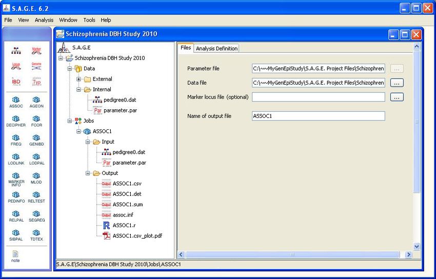
NOTICE

The recommended way of referencing the current release of the S.A.G.E. programs is as follows:
S.A.G.E. 6.4.1 [2021]. Statistical Analysis for Genetic Epidemiology http://darwin.cwru.edu.
You are requested to send bibliographic information to opensagecwru@gmail.com about every pa-
per in which S.A.G.E. is used (author(s), title, journal, volume and page numbers) to be posted in
https://github.com/elstonsage/SageCore/wiki/Publication, where you can find a list of papers by
other users of S.A.G.E. that we know of.

                                                1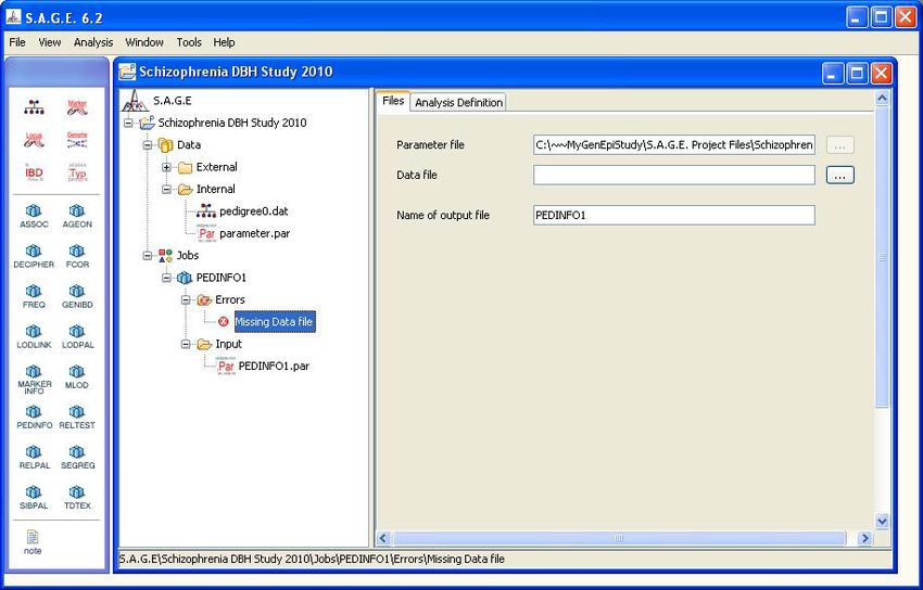
Contents

1   Creating a New S.A.G.E. Project                                                                    4
    1.1   Input Data Requirements . . . . . . . . . . . . . . . . . . . . . . . . . . . . . . .        4
    1.2   Start S.A.G.E. . . . . . . . . . . . . . . . . . . . . . . . . . . . . . . . . . . . . .     5
    1.3   Importing Pedigree Data . . . . . . . . . . . . . . . . . . . . . . . . . . . . . . .        7

2   Running the S.A.G.E. Programs                                                                     17
    2.1   Setting the Text Editor . . . . . . . . . . . . . . . . . . . . . . . . . . . . . . . .     17
    2.2   Using the Navigation Window . . . . . . . . . . . . . . . . . . . . . . . . . . . .         17
    2.3   Output Files . . . . . . . . . . . . . . . . . . . . . . . . . . . . . . . . . . . . . .    21

3   Genome Map File Wizard                                                                            24
    3.1   Supported Map Information . . . . . . . . . . . . . . . . . . . . . . . . . . . . .         24
    3.2   Importing a Genome Map File . . . . . . . . . . . . . . . . . . . . . . . . . . . .         24

4   Function Block Wizard                                                                             32
    4.1   Supported Actions . . . . . . . . . . . . . . . . . . . . . . . . . . . . . . . . . .       32
    4.2   Adding a New Function Block . . . . . . . . . . . . . . . . . . . . . . . . . . . .         33

5   GMDR Utility                                                                                      36
    5.1   Running . . . . . . . . . . . . . . . . . . . . . . . . . . . . . . . . . . . . . . . .     36
    5.2   Output Files . . . . . . . . . . . . . . . . . . . . . . . . . . . . . . . . . . . . . .    38

6   SNPCLIP                                                                                           40
    6.1   Limitations . . . . . . . . . . . . . . . . . . . . . . . . . . . . . . . . . . . . . .     40
    6.2   Theory . . . . . . . . . . . . . . . . . . . . . . . . . . . . . . . . . . . . . . . . .    40
          6.2.1   Dimension Reduction       . . . . . . . . . . . . . . . . . . . . . . . . . . . .   40
          6.2.2   Filters . . . . . . . . . . . . . . . . . . . . . . . . . . . . . . . . . . . . .   40
                  6.2.2.1    Missingness Filter . . . . . . . . . . . . . . . . . . . . . . . . .     41

                                                   2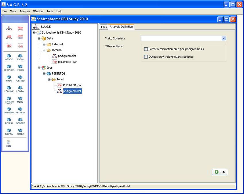
CONTENTS                                                                                CONTENTS

                6.2.2.2    Minor Allele Frequency Filter . . . . . . . . . . . . . . . . . . .     41
                6.2.2.3    Linkage Disequilibrium Filter . . . . . . . . . . . . . . . . . . .     41
                6.2.2.4    Genome Map Filter . . . . . . . . . . . . . . . . . . . . . . . .       41
        6.2.3   MUGS . . . . . . . . . . . . . . . . . . . . . . . . . . . . . . . . . . . .       41
  6.3   Running SNPCLIP . . . . . . . . . . . . . . . . . . . . . . . . . . . . . . . . . .        41
        6.3.1   Importing A Data File . . . . . . . . . . . . . . . . . . . . . . . . . . . .      42
        6.3.2   Importing A Map File . . . . . . . . . . . . . . . . . . . . . . . . . . . .       44
  6.4   Filtering a Data Set . . . . . . . . . . . . . . . . . . . . . . . . . . . . . . . . . .   45
  6.5   Running MUGS . . . . . . . . . . . . . . . . . . . . . . . . . . . . . . . . . . . .       48
  6.6   Exporting a Data Set . . . . . . . . . . . . . . . . . . . . . . . . . . . . . . . . .     52
  6.7   References . . . . . . . . . . . . . . . . . . . . . . . . . . . . . . . . . . . . . . .   53

                                                 3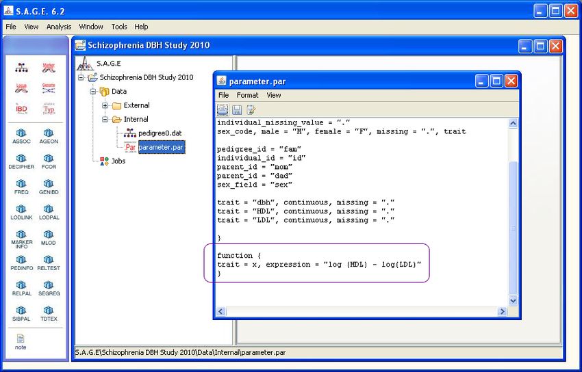
Chapter 1
Creating a New S.A.G.E. Project
This section provides general instructions for creating a new S.A.G.E. project using the GUI.
1.1 Input Data Requirements
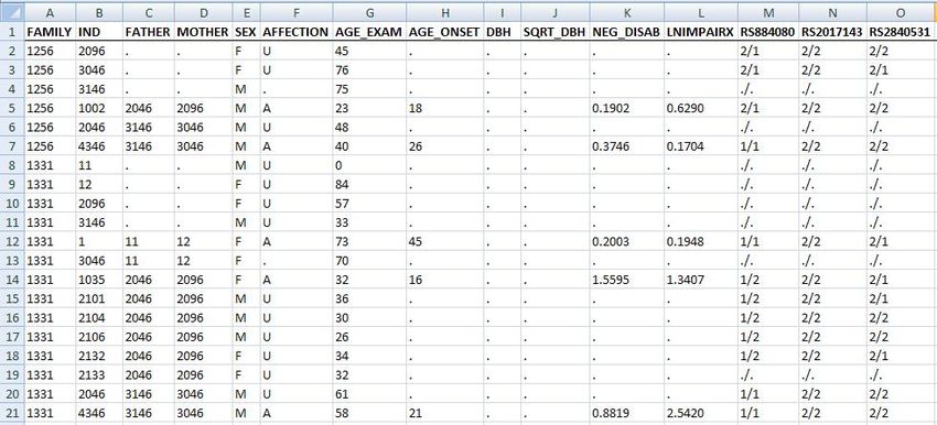
The S.A.G.E. programs require input data (i.e., your pedigree file) to be a delimited ASCII text
file or Excel spreadsheet in which each line of the file contains information on a single individual,
as shown in Figure 1.1 below. The example shows a portion of an Excel spreadsheet containing
pedigree sample data. Each row represents a different individual and each column represents a
different field or attribute of the individual. The first row contains the names of the fields. Field
names are entirely up to the user and need not be identical to those shown in the example; however
only letters, numbers and the underscore (“_”) character are permitted in field names.
The sample shown in Figure 1.1 will be interpreted by the S.A.G.E. software as follows (ID is an
abbreviation for “identifier”):
• Column 1 (FAMILY): identifies the pedigree to which the individual belongs. The exam-
ple shows 6 individuals who all belong to the pedigree designated as 1256. The coding for
the pedigree ID may be any combination of numbers, letters and printable characters, hence
“PED-2345” would be a valid pedigree ID.
• Column 2 (IND): uniquely identifies the individual within a given pedigree. The pedigree ID
and individual ID, taken together, must be unique within the entire data file. The coding for
individual ID may be any combination of numbers, letters and printable characters.
• Column 3 (FATHER): identifies the individual’s paternal parent
• Column 4 (MOTHER): identifies the individual’s maternal parent. Parental IDs are used to
establish family relationships among pedigree members. Every individual in the pedigree
data file must have either two parents or none. The period (“.”) character is used to indicate
a missing value for the parental identifier in Figure 1, but this can be changed, as indicated
later. An individual with no parents specified is considered to be either a founder or marry-in.
Thus with respect to family 1256, individual 1002 has mother: 2096 and father: 2046.
• Column 5 (SEX): The individual’s sex. Coding for sex is at the user’s discretion; typical
schemes are “M” and “F” (the default) or “1” and “0”.
4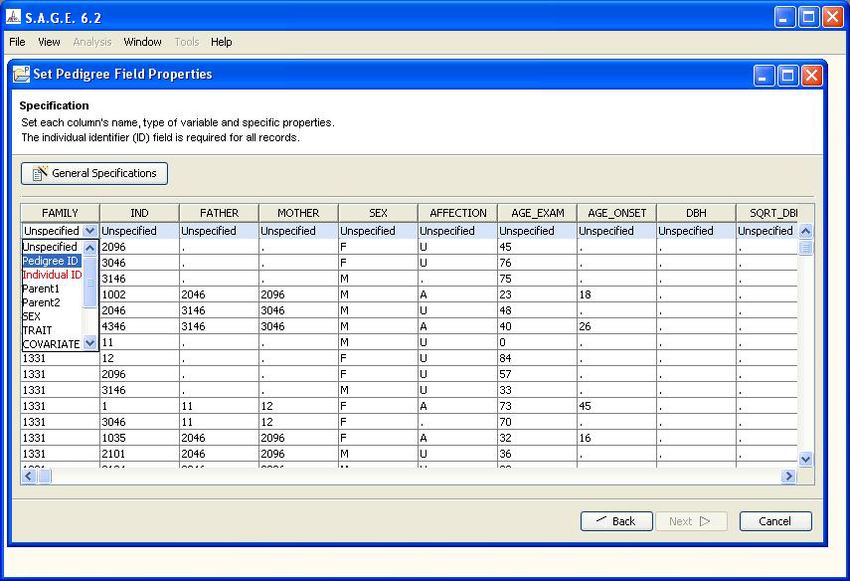
1.2. START S.A.G.E.                        CHAPTER 1. CREATING A NEW S.A.G.E. PROJECT

   • Columns 6 - 12 (various traits and covariates): These columns record the individual’s specific
     trait and/or covariate values with respect to the trait or disease of interest. Data types may be
     binary (for affected/unaffected status) or quantitative. Coding for a binary trait is at the user’s
     discretion; typical schemes are “A” and “U”, “1” and “0”, etc. The missing value character
     (“.”) is used to indicate that the information is unknown for a given individual in Figure 1,
     but again, this can be changed..

   • Columns 13 - 15 (marker phenotypes): These columns record the individual’s specific marker
     phenotypes (sometimes referred to as genotype, on the assumption that there is a one-one
     relation between marker phenotypes and genotypes) with respect to specific markers along
     the human genome. Each marker phenotype is encoded as the combination of two alleles
     delimted by the slash (“/”) character. Alleles may be encoded as any combination of letters
     and numbers, and the choice of delimiters is also flexible. Note that every marker locus must
     show either two alleles or none. The missing allele character (in this example, “.”) is used to
     indicate that the individual’s genetic information is unknown for a given location.

                                   Figure 1.1: Input Data Format

1.2    Start S.A.G.E.

On Windows platforms, double-click the S.A.G.E. icon to run the GUI, and on Linux platforms you
will need invoke the GUI through the standard Java interface. When the Setup dialog appears, select
Create new project to start (see Figure 1.2).

                                                  5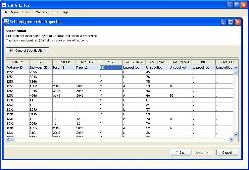
1.2. START S.A.G.E.                     CHAPTER 1. CREATING A NEW S.A.G.E. PROJECT

                                    Figure 1.2: Setup Dialog

When you click the “OK” button, you will see a New Project dialog, so that you can proceed.

                                               6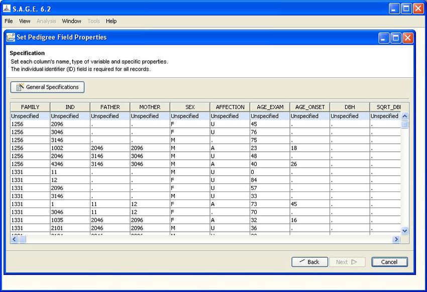
1.3. IMPORTING PEDIGREE DATA               CHAPTER 1. CREATING A NEW S.A.G.E. PROJECT

1.3    Importing Pedigree Data

This section describes the process of importing pedigree data into the S.A.G.E. project environment.
From the S.A.G.E. Main Menu bar, select File -> New Project. When the New Project dialog
appears, enter a name for your project such as “Schizophrenia DHB Study 2010” and select a
project location directory. S.A.G.E. will create a new project folder within the directory you specify
and store all relevant files at that location (see Figure 1.3).

                                  Figure 1.3: New Project Dialog

When you click the “Next” button, you will see a dialog that presents three options and your choice
depends on what kind of input files you have already prepared to use with S.A.G.E. If you have
correctly prepared and formatted your pedigree data file as described in Chapter 3 of the S.A.G.E.
User Reference Manual, then select the middle option and click the “Next” button (see Figure 1.4).

                                                  7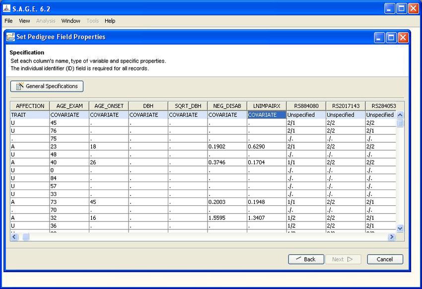
1.3. IMPORTING PEDIGREE DATA               CHAPTER 1. CREATING A NEW S.A.G.E. PROJECT

                             Figure 1.4: S.A.G.E. Import Mode Dialog

The next dialog requires you to enter the location of the pedigree data file you wish to import into
S.A.G.E. (Figure 1.5). In addition, you must provide some information about the file format. If
your data is contained within an Excel spreadsheet, you may simply click that option and proceed.
If your data is stored within an ASCII text file, then you must specify the type of character used to
delimit the fields (i.e., columns) and whether or not the first row contains the field names (in which
case, the first row is referred to as a “header row”).

                                 Figure 1.5: Data Location Dialog

After you click on the “Next” button once again, a Data Specification window will appear (Figure
1.6). You may see a warning dialog stating that only a portion of the columns will be displayed.
This is normal for pedigree files that contains many hundreds (or thousands) of genetic marker fields
and it will not prevent you from successfully loading or analyzing your data.

                                                  8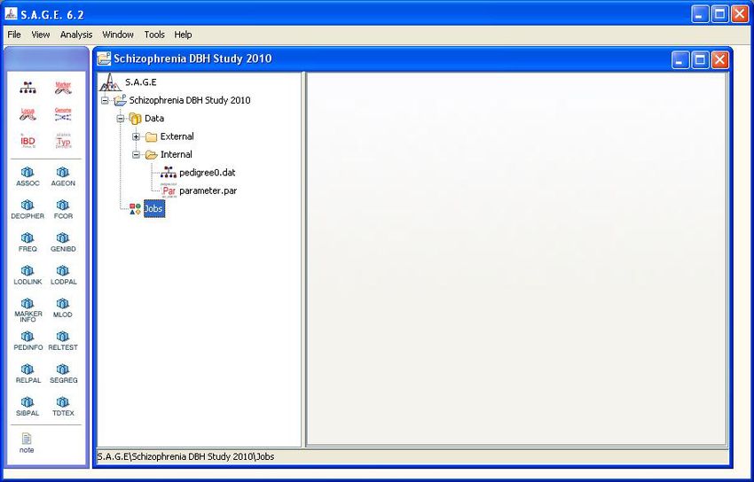
1.3. IMPORTING PEDIGREE DATA               CHAPTER 1. CREATING A NEW S.A.G.E. PROJECT

                              Figure 1.6: Data Specification Window

The Data Specification Window displays the rows and columns found in the original data file, along
with the field names inferred from the header row (if provided). Your task at this point is to fully
specify the semantics of each column so that the data may be correctly interpreted by S.A.G.E.
programs. For example, although the first column is labeled “FAMILY”, the S.A.G.E. software has
no prior way of knowing that the column actually represents a pedigree identifier. You specify that
bit of semantic information as follows:

   1. Click on the shaded cell containing the word “Unspecified” at the top of the column to make
      the drop-down arrow appear

   2. Click on the drop-down arrow to obtain a list of valid “data type” choices for the column

   3. Scroll down the list as needed to highlight the desired choice and click to select it (see Figure
      1.8). Possible data type choices are:

         • Unspecified (default): if this is selected, the column will NOT be imported into the
           S.A.G.E. environment
         • Pedigree ID: means the column represents a family identifier
         • Individual ID: means the column represents an individual identifier
         • Parent1: means the column represents a parental identifier (maternal or paternal)
         • Parent2: means the column represents a parental identifier (must be complementary to
           Parent1)
         • SEX: means the column represents the individual’s sex code
         • TRAIT: means the column represents a trait or phenotype presumed to have a heritable
           component that you will wish to analyze. May be binary or quantitative.

                                                  9
1.3. IMPORTING PEDIGREE DATA CHAPTER 1. CREATING A NEW S.A.G.E. PROJECT
• COVARIATE: means the column represents an arbitrary biometric, predictor or explana-
tory variable. (You will have the opportunity to analyze this variable as a trait, should
you wish to do so.) May be binary or quantitative.
• MARKER: means the column represents a marker phenotype formatted as X delim Y,
where X and Y are values of alleles and delim is a single character delimiter. For exam-
ple, “a/b, a/a, 1/0, 124-88, A~G, ...”
• ALLELE: means the column represents a single allele with respect to some marker phe-
notype. In such a case, there must be two consecutive single-allele columns specified,
one for each of the two observed values at the locus.
• TRAIT MARKER: means the column represents some phenotype for which you will be
able to specify a monogenic model that is sufficiently described to allow it to be tested
for linkage with one or more markers. May be binary or quantitative.
• TEXT: means the column represents a label or other useful information that is not suit-
able for numerical analysis.
Figure 1.7: Data Type Specification
101.3. IMPORTING PEDIGREE DATA CHAPTER 1. CREATING A NEW S.A.G.E. PROJECT
After specifying the data type of the first five columns, the display will look as shown in Figure 1.8.
There are two important points to remember here. First, the order of the columns does not matter.
For example, it is perfectly acceptable if your data file has the “SEX” column at some location other
than column #5.
The second noteable point is that the columns 1 - 5 as shown contain the essential structure infor-
mation for pedigree analysis: pedigree ID, individual ID, mother ID, father ID and sex. These five
items are the minimal requirement for almost all of the S.A.G.E. programs, so be sure your data
has this information before you try to import the file. (Please refer to the S.A.G.E. User Reference
Manual for the specifics.)
Note that the column names at the top have been taken directly from the header row of your input
file. These names will become the “variable” names that you can use within S.A.G.E. programs. If
you would like to change a name for some reason, for example change “FATHER” to “DAD_ID”,
simply double-click on the name and edit the field as desired.
Figure 1.8: Data Type Specification (continued)
111.3. IMPORTING PEDIGREE DATA CHAPTER 1. CREATING A NEW S.A.G.E. PROJECT
Column #6, designated “AFFECTION” represents a binary trait under study. When you select the
TRAIT data type from the drop-down list, a dialog appears as shown in Figure 1.9. The dialog
requires you to provide additional information about the data item. In particular you must specify
the character used to represent a missing value (a dot (“.”) by default), whether it is binary or
quantitative, and what values are associated with affected and unaffected status, respectively.
Figure 1.9: Variable Characteristics
121.3. IMPORTING PEDIGREE DATA CHAPTER 1. CREATING A NEW S.A.G.E. PROJECT
The next 6 columns in the example are set as quantitative covariates with default missing value char-
acter equal to “.”. When a pedigree data file contains multiple quantitative traits and/or covariates,
it is conventional to format the file such that the these columns have the same missing value. When
the data file has been prepared this way, the S.A.G.E. GUI provides a shortcut to specify all the traits
and/or covariates at once. At the bottom of the dialog is a check box labelled “Apply to next ___
column(s)”. If you check this box, then all of the subsequent columns (as indicated by the number
that appears in the box next to it) will be given the same data specifications (except for the Name
attribute).
Figure 1.10: Data Type Selection (continued)
131.3. IMPORTING PEDIGREE DATA CHAPTER 1. CREATING A NEW S.A.G.E. PROJECT
Select the MARKER type from the drop-down list for the first marker, and click the “OK” button
on the subsequent dialog to indicate that the marker is codominant (see Figure 1.11). You can
change the default allele delimiter and missing value characters if needed. At the bottom of the
dialog is a check box labelled “Apply to next ___ column(s)”. If you check this box, then all of the
subsequent columns (as indicated by the number that appears in the box next to it) will be given the
same data specifications (except for the Name attribute). When a pedigree data file contains marker
phenotypes, it is conventional to format the file such that the marker columns all occur after the
family structure and biometric data. When the data file has been prepared this way, you can use this
shortcut to specify all the markers at once.
Figure 1.11: Variable Characteristics (continued)
141.3. IMPORTING PEDIGREE DATA CHAPTER 1. CREATING A NEW S.A.G.E. PROJECT
Lastly, you must click on the “General Speci
cations” button to provide a remaining bit of informa-
tion (see Figure 1.12). If your data are already formatted with the default values for missingness and
sex code (as shown), then click the “OK” button to save the settings and close the dialog. Otherwise,
make the required changes.
Figure 1.12: Variable Characteristics (continued)
151.3. IMPORTING PEDIGREE DATA CHAPTER 1. CREATING A NEW S.A.G.E. PROJECT
Click the “Next” button at the bottom of the Data Specification window to complete the import
process. Accept the default value for the imported file name (unless you have a preference for a
different name) and, after the data has been successfully imported, the main S.A.G.E. navigation
window and tool palette will be displayed as shown in Figure 1.13. Note: The data import process
makes a copy of your original data file (minus any columns that have been left unspecified) and
stores the copy within the S.A.G.E. project directory previously generated by the program.
Figure 1.13: Main Navigation Window
16Chapter 2
Running the S.A.G.E. Programs
This section describes how to run S.A.G.E. programs and reviews their various output files.
2.1 Setting the Text Editor
When S.A.G.E. programs run, they produce ASCII text files as output. Further, the imported data
file and other input files used by S.A.G.E. are also text files. Since you will need to be able to
view and edit those files on occasion, the S.A.G.E. GUI provides a very simple text editor for that
purpose. However, you may wish to use a more powerful editor, especially to view large data files,
in which case you can specify the editor of your choice from the Tools -> Preferences menu in the
main window. When the Preferences dialog appears, click on the “Browse” button to select the
executable file for the text editor you want to use with S.A.G.E. Be sure to select a proper text editor
and NOT a word processing program such as Microsoft Word. There are many good text editors
available, and we recommend one called TextPad (www.textpad.com).
2.2 Using the Navigation Window
The first step in running S.A.G.E. programs is to verify that the data were imported correctly. This is
best accomplished by running the PEDINFO (Pedigree Information) program. Any of the S.A.G.E.
programs can be launched by one of three means:
1. Select the desired program from the Analysis Menu of the Main Window toolbar.
2. Right-click on the Jobs icon in the Navigation panel and select the desired program from the
list that appears.
3. Drag-and-drop the desired program icon from the palette onto the Jobs icon in the Navigation
panel (this is usually the quickest method)
Using one of these three methods, create a new PEDINFO job. The result should look similar to
Figure 2.1 shown below. Note that the Errors subfolder will contain an item called “Missing Data
File”. This is normal and it simply means that you must specify which internal data file you want to
172.2. USING THE NAVIGATION WINDOW
CHAPTER 2. RUNNING THE S.A.G.E. PROGRAMS
analyze with the PEDINFO program. Use the mouse to drag-and-drop the “pedigree0.dat” file from
the Internal folder onto the “Missing Data File” icon, and the error will be resolved. Alternatively,
you could click on the “...” button to the right of the “Data file” text field and browse to the file of
your choice. In general, however, it is better to simply use the drag-and-drop method.
Figure 2.1: A New PEDINFO Job
Lastly, click on the “Analysis Definition” tab to set any other desired options for the PEDINFO
program (see Figure 2.2).
182.2. USING THE NAVIGATION WINDOW
CHAPTER 2. RUNNING THE S.A.G.E. PROGRAMS
Figure 2.2: Setting PEDINFO Options
Before running the program, there are a few points worth noting.
1. The default label for the new job (i.e., S.A.G.E. program task) is called “PEDINFO1”. You
can change the name by clicking once on the label to place it into edit mode.
2. To delete a job from those listed in the Navigation panel, right-click on the job’s icon and then
select “Delete” from the list.
3. To view and/or edit the contents of any of the files listed within the job subfolders, simply
double-click to invoke the text editor.
The file named “PEDINFO1.par” is the S.A.G.E. parameter file created for the job. A parameter
file is simply a text file containig information about the pedigree data file and user options neeeded
to run a particular program (see Figure 2.3). When a S.A.G.E. program runs, it reads the parameter
file to acquire specifications on how to interpret the data file, and then loads the data file itself. After
the data file has been loaded into memory, the program applies whatever user options are specified
to complete the job. In the example below, the PEDINFO job appears to have no options specified,
which means that the program will simply run with whatever default behavior had been programmed
into it.
192.2. USING THE NAVIGATION WINDOW
CHAPTER 2. RUNNING THE S.A.G.E. PROGRAMS
Figure 2.3: Parameter File
When you click on the “Run” button to launch a S.A.G.E. program (PEDINFO, in this example), the
“Analysis Information” dialog appears as shown in Figure 2.4. The dialog allows you to preview
the parameter file settings that have been created as a result of the GUI options you selected. If
necessary, you can make changes directly through this dialog before running the program.
Figure 2.4: Analysis Information
When you click on the “OK” button, the GUI will launch the selected S.A.G.E. program. Runtime
202.3. OUTPUT FILES CHAPTER 2. RUNNING THE S.A.G.E. PROGRAMS
output from the will be displayed within a Console window, and elapsed time information will be
displayed within a Tasks window (see Figures 2.5 and 2.6).
Figure 2.5: Console Window
Figure 2.6: Tasks Window
2.3 Output Files
When the program has completed executing the job, an “Output” subfolder will contain all of the
files produced by the S.A.G.E. program (see Figure 2.7).
212.3. OUTPUT FILES CHAPTER 2. RUNNING THE S.A.G.E. PROGRAMS
Figure 2.7: Output Files
Double-click on any of the output files to view their contents. Most importantly, you should AL-
WAYS view the *.inf file (“pedinfo.inf”, in this case). It contains informational diagnostic mes-
sages, warnings and program errors. EXAMINE THIS FILE FIRST BEFORE OPENING ANY
OTHER ANALYSIS OUTPUT FILES.
If any of the regular analysis output files are needed by other S.A.G.E. programs, you may simply
drag-and-drop them onto the target job subfolders as needed.
222.3. OUTPUT FILES CHAPTER 2. RUNNING THE S.A.G.E. PROGRAMS
With ASSOC, SIBPAL, and LODPAL jobs, the GUI produces an R script file and a pdf file with the
resulting plot(s) (see Figure 2.8) in addition to the regular analysis output files. The user can modify
this R script file to produce a more desirable plot running R outside of the GUI.
Figure 2.8: Result Plots
23Chapter 3
Genome Map File Wizard
This section describes how to use the Genome Map File Wizard tool in the GUI to prepare a
S.A.G.E. compatable genome map file. When a S.A.G.E. program requires a genome map file,
you can run the Genome Map File Wizard to correcly format your gemone map file into a S.A.G.E.
compatable genome map file.
3.1 Supported Map Information
The Genome Map File Wizard supports four different map information types to be imported into
the S.A.G.E. GUI to generate a S.A.G.E. compatable genome map file.
1. Position in the genetic map from p-ter
2. Absolute position in the physical map (base pair)1
3. Distance in centimorgans(cM) to the next marker2
4. Recombination fraction to the next marker
A raw genome map information file can be either a delimited ASCII text file or an Excel spreadsheet
in which each line of the file contains information on a single marker.
3.2 Importing a Genome Map File
From the S.A.G.E. Main Menu bar, select Tools -> Create a Genome Descreption File. When the
Genome map file wizard dialog appears, enter the location of your raw genome map information
file with appropriate information for your file format (see Figure 3.1).
1 Note that this physical position is translated into a genetic distance in cM on the (false) assumption that 1,000,000
base pair corresponds to 1 (Haldane or Kosambi) cM.
2 Note that the output from a linkage run then starts at the first marker.
243.2. IMPORTING A GENOME MAP FILE CHAPTER 3. GENOME MAP FILE WIZARD
Figure 3.1: Data Location Dialog
Click the “Next” button at the bottom of the Import Genome Data window to specify the map
function (see Figure 3.2). Enter the name of the genome and select the appropriate map function for
your analysis, then click the “Next” button at the bottom for the next step.
Figure 3.2: Map Function Specification Dialog
253.2. IMPORTING A GENOME MAP FILE CHAPTER 3. GENOME MAP FILE WIZARD
On the next step, a Data Specification Dialog appears (see Figure 3.3). The Data Specification
Dialog displays the rows and columns found in the original genome map data file, along with the
field names inferred from the header row (if provided).
1. Click on the shaded cell containing the word “Unspecified” at the top of the column to make
the drop-down arrow appear.
2. Click on the drop-down arrow to obtain a list of valid “data type” choices for the column.
3. Scroll down the list as needed to highlight the desired choice and click to select it. Possible
data type choices are:
• Unspecified (default): if this is selected, the column will NOT be imported into the
S.A.G.E. environment
• Marker: means the column represents a marker name
• Position: means the column represents position information
Figure 3.3: Map Data Specification Dialog
263.2. IMPORTING A GENOME MAP FILE CHAPTER 3. GENOME MAP FILE WIZARD
When you select Position from the drop-down list, a position information specification dialog ap-
pears as shown in Figure 3.4.
Figure 3.4: Position Information Specification Dialog
After you select the columns to import with the proper data type specification (Figure 3.5), click the
“Next” button at the bottom for the next step.
Figure 3.5: Map Data Specification Dialog (continued)
273.2. IMPORTING A GENOME MAP FILE CHAPTER 3. GENOME MAP FILE WIZARD
In the next step, a Region information Specification Dialog appears (see Figure 3.6).
Select markers by clicking the first marker and then clicking the last marker while holding down the
shift key (alternatively, the marker range can be selected by dragging the cursor over the markers).
Then click the “Set Region” button and type in the region name for the selected markers (Figure 3.7
and 3.8).
Figure 3.6: Region Information Specification Dialog
283.2. IMPORTING A GENOME MAP FILE CHAPTER 3. GENOME MAP FILE WIZARD
Figure 3.7: Region Information Specification Dialog (continued)
Figure 3.8: Region Information Specification Dialog (continued)
293.2. IMPORTING A GENOME MAP FILE CHAPTER 3. GENOME MAP FILE WIZARD
After specifying the Regions correctly for all markers, click the “Next” button at the bottom, and
then enter the name of the newly imported file (Figure 3.9).
Figure 3.9: Filename Specification Dialog
303.2. IMPORTING A GENOME MAP FILE CHAPTER 3. GENOME MAP FILE WIZARD
After the genome map data have been successfully imported, you can see the new file under the
“internal” folder in the main S.A.G.E. navigation window as shown in Figure 3.10.
Figure 3.10: Main Navigation Window
31Chapter 4
Function Block Wizard
This section describes how to use the Function Block Wizard tool in the GUI to create or modify
function blocks in a parameter file. This tool can be used at any time after the pedigree file has been
imported into a project.
4.1 Supported Actions
To start the Function Block Wizard tool, select Tools -> Create New Variable from the S.A.G.E.
Main Menu bar. When the function Specification Dialog appears (Figure 4.1), four possible actions
can be performed:
1. Add a new function block at the end of existing function blocks (if any)
2. Edit an existing function block
3. Delete an existing function block
4. Change the order of existing function blocks
Figure 4.1: Specification Dialog
If there exists any previous user-defined function blocks in the imported parameter file, they will be
displayed in this dialog.
324.2. ADDING A NEW FUNCTION BLOCK CHAPTER 4. FUNCTION BLOCK WIZARD
4.2 Adding a New Function Block
From the Specification Dialog above, click “Add” button to add a new function block. It will bring
up the Expression Dialog as shown in Figure 4.2.
Figure 4.2: Expression Dialog
This dialog requires you to enter the new variable name and select the appropriate attributes. All
constants, operators and elementary functions, as well as all existing variables that may be used in
the new function expression, are listed in this dialog. You can type in the new function expression
into the Expression window in Figure 4.3 (outlined in purple).
Figure 4.3: Expression Dialog (continued)
334.2. ADDING A NEW FUNCTION BLOCK CHAPTER 4. FUNCTION BLOCK WIZARD
You can also click the desired elements in order to compose the new function expression (see Figure
4.4 and 4.5).
Figure 4.4: Expression Dialog (continued)
Figure 4.5: Expression Dialog (continued)
After you select all the necessary elements for a function expression, click the “OK” button next to
344.2. ADDING A NEW FUNCTION BLOCK CHAPTER 4. FUNCTION BLOCK WIZARD
the Expression window to complete the adding process. This will bring back the main Specification
Dialog with the newly created variable and expression (Figure 4.6).
Figure 4.6: Specification Dialog
Again, click “OK” button in the Specification Dialog to complete and save the process.
Once the new function block has been successfully created, you can see it in the parameter file in
the main S.A.G.E. navigation window as shown in Figure 4.7 (outlined in purple).
Figure 4.7: Main Navigation Window
35Chapter 5
GMDR Utility
This section describes how to use the GMDR utility tool in the GUI to create input files for the Gen-
eralized Multifactor Dimensionality Reduction (GMDR) program (http://www.ssg.uab.edu/gmdr/)
using the output files from the ASSOC program. This tool can be used at any time after the ASSOC
output files has been generated in a project.
5.1 Running
To start the GMDR utility tool, select Tools -> GMDR Utility from the S.A.G.E. Main Menu bar.
The Main Screen for GMDR Utility appears (see Figure 5.1) showing three main panels: Required
files (top), Marker information (bottom left), and Class information (bottom right).
Figure 5.1: Main screen for GMDR Utility
365.1. RUNNING CHAPTER 5. GMDR UTILITY
Required files
• ASSOC parameter file – the location of the parameter file
• Pedigree file – the location of the pedigree data file
• ASSOC residual file – the location of the ASSOC residual output file
• ASSOC summary file – the location of the ASSOC summary output file
Marker information
After importing the required files above, the program will display all the available markers in the
file you imported by marker name (Figure 5.2. at bottom left) or by model (Figure 5.2. at bottom
left) in marker information panel.
For the genotype file, you should pick a small subset of them.
Figure 5.2: Markers by name
375.2. OUTPUT FILES CHAPTER 5. GMDR UTILITY
Figure 5.3: Markers by model
When the program parses marker name by model, it assumes that the model name is in the form
“xxx_valid marker name”, where x represents any letter or digit.
Class information
• Column – the column containing class information in the pedigree file.
• Affected value / Threshold – the value representing affected in the column. If the column
contains quantitative values, values greater than the threshold are considered to be affected.
5.2 Output Files
Click “OK” button, then this utility will create two files for GMDR.
• Genotype file
• Phenotype file
Once it has completed the process, the result dialog will pop-up in the center of your screen (see
Figure 5.4).
385.2. OUTPUT FILES CHAPTER 5. GMDR UTILITY
Figure 5.4: Result Dialog
The user can run the GMDR using these files.
Note:
The phenotype file will be independent residuals from a null model, as in ASSOC you must have
“model, null=true”. Because ASSOC allows adjustment for covariates, there is no need to do that
in GMDR (i.e. SCHEME2 is unnecessary).
39Chapter 6
SNPCLIP
SNPCLIP allows investigators to perform filtering on SNP data sets based on a set of statistical
calculations. The user can then output the dataset into S.A.G.E. format for further processing.
Currently, SNPCLIP allows investigators to filter based on missingness, allele frequency, pairwise
linkage disequilibrium, and genome map regions. A special feature allows the user to search the
Maximum Unbroken Genomic Sequences (MUGS) in a set of individuals, i.e., the largest haplotype
they might share.
6.1 Limitations
SNPCLIP currently supports SNPs with two alleles (or a missing value) at each location.
SNPCLIP’s memory usage has been optimized for usage with SNP data. The internal data format
is similar to that of PLINK. As an example of its effeciency, the program can store 19K SNPs over
162 individuals using only 50 MBs of RAM (Hapmap phase 3 data).
6.2 Theory
6.2.1 Dimension Reduction
Dimension Reduction is a term used to describe a filtering of a data set so that only relevant data
remain. SNPCLIP reduces the dimension of a data set by using any of the available filters provided
(missingness, allele frequency, etc.). By reducing the dimension (in this case, the number of SNPs)
of a data set one can eliminate elements of the data set that do not provide useful information or
have undesireable attributes. Two major benefits to reducing the dimensionality of a data set is that
the resulting data set contains only the data of interest, which in turn, reduces the amount of time to
perform further analysis on the data set.
6.2.2 Filters
Filtering is the core of SNPCLIP. It is a form of dimension reduction that allows the user to specify
restrictions on the data set to obtain useful SNPs. The term filtering is more appropriate in this
406.3. RUNNING SNPCLIP CHAPTER 6. SNPCLIP
setting because the user supplies a set of criteria that the data must comply with. All of the filters
within SNPCLIP are INCLUSIVE, meaning that any SNP that meets all the criteria specified will
remain in the filtered set.
6.2.2.1 Missingness Filter
The missingness filter takes a simple count of how many individuals have missing data for a given
SNP. If the percentage of missing individuals at a given SNP falls within the min and max values
specified by the user, they will be included in the filtered data.
6.2.2.2 Minor Allele Frequency Filter
The minor allele frequency filter counts the total number of occurrances of each allele for each SNP.
It then selects the allele at each SNP with the lower count as the minor allele. If the percentage of
minor alleles present at a given SNP falls within the min and max values specified by the user, then
the SNP will be included in the filtered data.
6.2.2.3 Linkage Disequilibrium Filter
The LD filter calculates the composite LD between each pair of adajacent SNPs (Weir 1996). It then
filters out SNPs that do not fall within the min and max specified by the user. Next, the LD filter
enters a loop, comparing the remaining SNPs. The filter will continue to apply the filter recursively
on the remaining SNPs until no change in the number of SNPs has occured between one run and
the subsequent run.
6.2.2.4 Genome Map Filter
The genome map filter filters the SNPs based upon the map specified by the user and the region(s)
and SNP(s) specified by the user in the map location dialog.
6.2.3 MUGS
Given a sequence of unphased diallelic SNP genotypes in a region for each of a set of N individ-
uals, MUGS searches for haplotype sequences that could be common to all N, or N-1, individuals
in the set, and then ranks them according to their length as defined by the number of SNPs in the
sequence. A SNP that is homozygous contributes to this length but gives no haplotype information.
Either allele of a heterozygous SNP can contribute to a common haplotype, so MUGS essentially
searches over all possible phases to find sequences that could be common to the N or N-1 individ-
uals. Although the individuals may be related, no relationship information is used. A SNP with a
mising value contributes to the sequence length.
6.3 Running SNPCLIP
To run SNPCLIP, locate and start the SNPCLIP.exe file in your S.A.G.E. directory or from the Start
Menu.
416.3. RUNNING SNPCLIP CHAPTER 6. SNPCLIP
Figure 6.1: Main Screen for SNPCLIP. Outlined in red is the file import button.
6.3.1 Importing A Data File
To import a file, click the “...” button (see Figure 6.1, outlined in red).
Figure 6.2: File Open Dialog
This will open a file browser (see Figure 6.2). Browse to the appropraite file and click the “Open”
button to begin the import process.
426.3. RUNNING SNPCLIP CHAPTER 6. SNPCLIP
Figure 6.3: File Information Dialog. Allows user to specify the format of the data file.
You will now have to specify information about the file format to SNPCLIP (see Figure 6.3).
First - Select your file format type.
• If each row represents an individual, with the columns representing SNPs, select the S.A.G.E.
format.
• If your file contains HapMap phase 3 data, select the Hapmap format.
• If each row represents a SNP, with columns representing individuals in the sample, select the
SNPs by Row format.
Second - Select the file delimiter.
• Select the appropriate delimiter from the list.
• If your delimiter is not listed, select the “other” option and specify it in the box provided.
• The data preview table will display the first few rows and columns of your file using the
delimiter specified. (This is a good way to check that you specified the correct delimiter).
Third - If you have pedigree data, specify where the identifier can be found.
• In the picture above the pedigree ID is specified in the first column (FAMID) and the Individ-
ual ID is specified by the second column (ID).
Fourth - Provide information about the file format.
• “Start SNP Column Data” should specify the column in which the SNP data begin.
– In the picture above the SNP data begin in the 13th column.
436.3. RUNNING SNPCLIP CHAPTER 6. SNPCLIP
• The delimiter in this menu is meant to represent the delimiter between allele values for a SNP
– In the picture above the delimiter is a “/” since each allele value is seperated by a “/”.
• The Missing value is meant to represent the missing value for an allele.
– In the picture above the missing value is set to “.”.
Fifth - Click the “OK” button.
SNPCLIP will now import your file to the system. You can see the import progress in the progress
bar dialog that will popup in the center of your screen. Once the progress bar reaches 100% the
file import process is completed. The dialog box will disappear and you will be left at the main
SNPCLIP screen.
Figure 6.4: Main Screen for SNPCLIP. Outlined in red are the information boxes.
SNPCLIP will display basic information regarding the data file you imported (outlined in red boxes
in Figure 6.4). The guage in the lower righthand corner of the screen gives the user a visual display
of how many SNPs remain after a set of filters have been applied.
At this point, you may begin filtering your data set (see section 6.4) or you may import a map file
for your data set (see section 6.3.2).
6.3.2 Importing A Map File
The user may also specify a map file by clicking the “...” button next to the Map File Path similar
to the Data File Path. Once this button is clicked, the following dialog will appear (Figure 6.5):
446.4. FILTERING A DATA SET CHAPTER 6. SNPCLIP
Figure 6.5: Map File Import Dialog
SNPCLIP accept two different formats, please select the approapriate format above. The examples
of these two formats are shown in Figure 6.6.
Figure 6.6: One line per marker (left) and two lines per marker (right)
Finally browse to the file and click “Open” button, similar to how the Data File was specified, and
you will be left at the main SNPCLIP screen again (Figure 6.7).
Figure 6.7: Main Screen for SNPCLIP after importing the map file
6.4 Filtering a Data Set
Once the file has completed the import process (see section 6.3.1), you will see a screen similar to
the one in Figure 6.7. In the source file area in the upper left hand portion of the window aspects
456.4. FILTERING A DATA SET CHAPTER 6. SNPCLIP
about the data file are imported.
In this case the data files has 5540 SNPs for 921 individuals.
You can now proceed to filtering the SNPs.
Click the check box of the filters that you would like to use (see Figure 6.8). You can see in this
figure, the user has selected the “Missingness” and “Minor Allele Frequency” filters (outlined in
red).
The “Min” and “Max” values represent the filtering criteria for the filter (see section 6.2.2 for details
on each filter).
The SNPs that have values that fall within the min and max will be kept, the remainig SNPs will be
clipped (filtered) out.
Click the “Apply” button once you are satified with your choices for filtering.
Figure 6.8: Specifiying a Filter
The progress bar will display SNPCLIP’s filtering progress. Once the filtering is complete you will
notice a tab in the results section specifying how many SNPs are remaining, the filters applied, and
the values for the min/max (see Figure 6.9).
The beauty of storing filter information in tabs is that you can have multiple tabs open at once and
easily compare how different filters affected the data set reduction.
You will also notice in the lower right hand corner the SNP count and percent remaining (relative to
the original data set) are provided.
466.4. FILTERING A DATA SET CHAPTER 6. SNPCLIP
Figure 6.9: Main Screen for SNPCLIP after applying a filter
It is also possible to filter the data set by genome map region. The user can open the map location
dialog by clicking the check box next to the genomic region option at the end of the filters and then
clicking the “...” button. Once the menu is open (see Figure 6.10), the user can add regions and/or
SNPs that they wish to include in the filter.
Figure 6.10: Genome Map Location Filter Dialog
If the user selects a region, they may further specify the precise location(s) within the region that
they would like by clicking the “Location Details” button.
476.5. RUNNING MUGS CHAPTER 6. SNPCLIP
Figure 6.11: Location Detail Dialog
The location details dialog (see Figure 6.11) allows the user to specify the range of locations they
would like to include via two drop down menus. The user needs to specify the location regions for
each region individually. If no location details are specified for a given region, all the SNPs within
the region will be included in the filter. Once all the selections have been made, simply click the
“OK” button on the map location dialog.
You may continue to apply filters to the data set until you find the proportion of remaning SNPs you
are looking for.
6.5 Running MUGS
Once SNPCLIP has completed the import process, you will see a screen similar to the one in Figure
6.12.
Figure 6.12: Main Screen for SNPCLIP after importing the files
From the SNPClip Main Menu bar, select Tools -> MUGS. The Main Screen for MUGS will appear
as in Figure 6.13.
486.5. RUNNING MUGS CHAPTER 6. SNPCLIP
Figure 6.13: Main Screen for MUGS
This dialog allows the user to specify either one or two different groups of criteria for computation.
MUGS without any group criteria
You can see the initial sample size (i.e. number of individuals) in your file at the bottom of the
group1 criteria window (see Figure 6.14). To display the MUGS result for the default option (i.e.
for all individuals), click the “Go” button.
Figure 6.14: MUGS result without criteria
496.5. RUNNING MUGS CHAPTER 6. SNPCLIP
MUGS with criteria for group
It is also possible to display the MUGS results for a set of group criteria, and for up to two different
groups with different criteria in each. Let’s assume that we want to compare affected and unaffected
individuals. Once you set the criteria for a group, the sample size will be updated (see Figure 6.15,
outlined in orange, at left). To display the MUGS results for one of the groups, click the “Go” button
for that group.
Figure 6.15: MUGS result with criteria for two groups (though not illustrated here, there may be
multiple criteria for a group)
Notice the longest SNP sequence window in Figure 6.14 and Figure 6.15 at center. Each block
represents one SNP.
• Cyan – SNP that is common to all N individuals
• Magenta – SNP that is common to at least N-1 individuals
• Yellow – Homozygote SNP
• Gray – None of the above
The program allows the user to specify a "broken-ness threshold" in the Collective Agreement panel
(Figure 6.15, outlined in green, at top right) as follows: If N individuals are submitted in the group
for analysis, then by default the algorithm will attempt to find unbroken genotype sequences that
are common to N individuals in the group. However, the user may optionally relax that constraint
to N-1, in which case the algorithm will attempt to find unbroken sequences that are common to at
least N-1 of the individuals in the group.
The program also allows the user to search for specific SNPs (Figure 6.15, outlined in violet, at
right). If the user enters a comma separated list of SNPs, it will display for each SNP a sequence
506.5. RUNNING MUGS CHAPTER 6. SNPCLIP
containing that SNP and a sequence containing all of the SNPs in the list. When the user clicks a
sequence ID in the search result, the program automatically highlights the sequence in the longest
SNP sequence window.
The “All SNP Visualization” panel (Figure 6.15, outlined in red, at bottom center) shows the results
for all SNPs in your data. You can use the scroll bar to move to a specific position you have interest
in. The zoom buttons allow the user to magnify the regions. When the user clicks the specific
position in the “All SNP Visualization” panel, the program automatically highlights the sequence in
the longest SNP sequence window.
For each sequence of SNPs, you can see more information by right clicking on a sequence and
selecting “Show details” as in Figures 6.16. Then the detail dialog will show the allele frequency
and missing individuals for each SNP as in Figure 6.17.
Figure 6.16: Right click on SNP sequence to display detail dialog
Figure 6.17: Details of Group1 and Group2
516.6. EXPORTING A DATA SET CHAPTER 6. SNPCLIP
Click the “OK” button (bottom right of the main screen for MUGS) to save the MUGS result as a
filtered data set in SNPCLIP (see Figure 6.18). SNPCLIP also allows the user to select a specific
format for outputting these data by clicking on File -> Export (see next section).
Figure 6.18: Main Screen for SNPCLIP after MUGS
6.6 Exporting a Data Set
SNPCLIP allows the user to output the filtered data set in S.A.G.E. format, Affymetrix format, or
both at the same time. You can reach the export feature by clicking File -> Export. The following
dialog will appear on your screen:
Figure 6.19: Export File Dialog
Pick the appropraite output format and click “OK”. Next specify the filename and location you
would like the data to be exported too. The S.A.G.E. formated file will be named with the file name
you supplied; the Affymetrix formated file wll be named with the file name you supplied with a
“_T” appended to the end of it.
526.7. REFERENCES CHAPTER 6. SNPCLIP
6.7 References
Weir, Bruce (1996), Genetic Data Analysis II, 125-127.
53You can also read