Stock Market Reactions to the COVID-19 Pandemic
←
→
Page content transcription
If your browser does not render page correctly, please read the page content below
Stock Market Reactions
      to the COVID-19 Pandemic
                     Steven J. Davis
              Academic Keynote Talk,
            ABFER 8th Annual Conference
                         25 May 2021

This talk draws on research with Scott Baker, Nick Bloom, Stephen
Hansen, Kyle Kost, Dingqian Liu, Marco Sammon, Cristhian
Seminario-Amez, Xuguang Simon Sheng, and Tasaneeya Viratyosin.
Some Context
1. Tremendous stock market reactions to COVID-19:
  – Globally, stocks fell 40% from 17 Feb. to 23 March 2020.
  – Too big to rationalize with a standard asset-pricing model.
  – One of the great volatility episodes in the past 120 years.
  – More daily U.S. stock market moves > |2.5%| in March 2020
     than any month since 1900.
2. No previous pandemic, including the Spanish Flu, had remotely
   similar stock market effects in the United States or China.
3. Huge dispersion in firm-level equity return reactions to market-
   moving news in Feb-March 2020.
  – Re COVID-19 as a reallocation shock, see Barrero, Bloom and
     Davis (2020, 2021ab) and Schmidt and Papanikalaou (2021).   1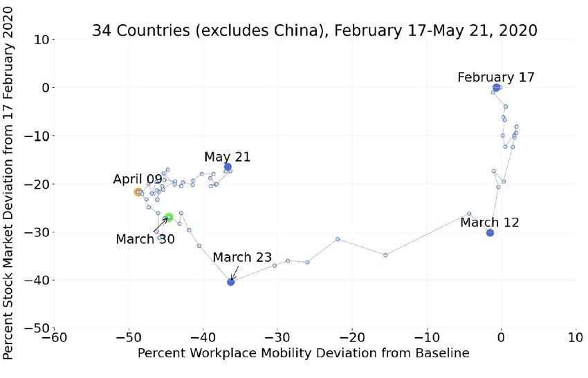
Only China, Taiwan and South Korea
depart materially from this pattern.

                      Reproduced from Davis, Liu and Sheng (2021).

                                                                2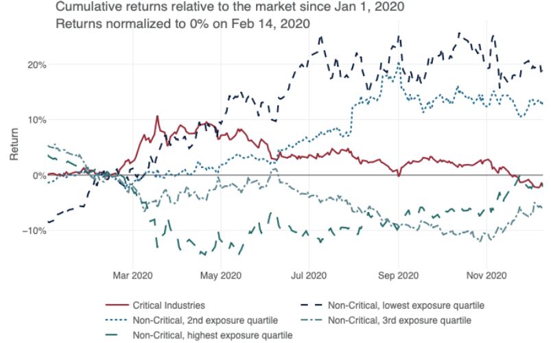
Realized U.S. Stock Market Volatility, January 1900 to April 2020
Volatility Last Two Weeks (1900-2020) Black
0.07 Great Crash Monday Coronavirus
10-11/1929 10/1987 Pandemic
0.06 3/2020
Great Global
0.05 Depression Financial
0.04 3/1933 Crisis
0.03 12/2008
0.02
0.01
0.00
2-Jan-00
1-Jan-03
1-Jan-06
1-Jan-09
1-Jan-12
1-Jan-15
1-Jan-18
1-Jan-21
1-Jan-24
1-Jan-27
1-Jan-30
1-Jan-33
1-Jan-36
1-Jan-39
1-Jan-42
1-Jan-45
1-Jan-48
1-Jan-51
1-Jan-54
1-Jan-57
1-Jan-60
1-Jan-63
1-Jan-66
1-Jan-69
1-Jan-72
1-Jan-75
1-Jan-78
1-Jan-81
1-Jan-84
1-Jan-87
1-Jan-90
1-Jan-93
1-Jan-96
1-Jan-99
1-Jan-02
1-Jan-05
1-Jan-08
1-Jan-11
1-Jan-14
1-Jan-17
1-Jan-20
0.06
0.05
0.04
0.03
Volatility Last Two Weeks (January 2020-April 2020)
0.02
0.01
0
20
0
20
20
20
0
20
20
20
20
0
9
0
0
0
0
0
0
-2
-2
-2
-2
-2
-2
r-2
-2
-2
-1
n-
n-
n-
n-
n-
-
-
-
ec
b
pr
pr
pr
ar
ar
ar
ar
eb
eb
eb
Ap
- Ja
- Ja
- Ja
- Ja
Ja
Fe
-M
-M
-M
-A
-A
-A
M
-D
-F
-F
-F
3-
3-
7-
10
17
24
31
6-
10
17
24
14
21
28
27
13
20
27
Notes: The sample period runs from 1/2/1900 to 4/30/2020. From December 1925 onwards, returns are computed using
Yahoo Finance’s ‘adjusted close’ series for the S&P 500 (^GSPC). Before that, returns are from the Global Financial Data
extension of the Dow Jones Index. In both panels, we calculate realized volatility as the sum of squared returns over the 3
past 10 trading days. Reproduced from Baker, Bloom, Davis, Kost, Sammon and Virayosin (2020).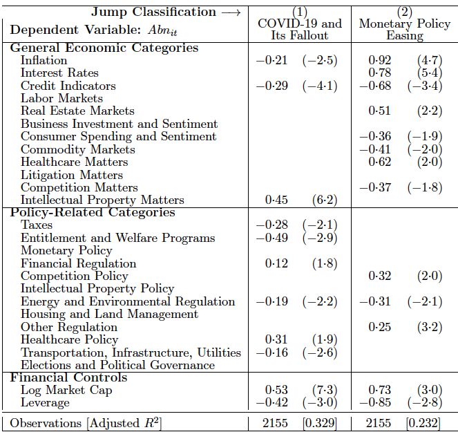
The Unprecedented Stock Market Impact of the Coronavirus
                          Number of Daily U.S.         Number Attributed to          Number Attributed
                          Stock Market Jumps             Economic Fallout            to Policy Responses
                          Greater than |2.5%|              of Pandemics                 to Pandemics

   2 January 1900 to
   21 February 2020                1,116                           0                            0
    24 February 2020
     to 30 April 2020                27                          13.4                         10.4
Note: Tabulated from results in Baker, Bloom, Davis and Sammon (2020), who consider all daily jumps in the U.S.
stock market greater than 2.5%, up or down, since 1900. They classify the reason for each jump into 17 categories
based on human readings of next-day (or same-evening) accounts in the Wall Street Journal (and New York Times
in 2020). Fractional counts arise when newspapers differ in their jump attribution or human readers differ in their
classification of the attribution. Number Attributed to Economic Fallout of Pandemics includes jumps on 3/12 and
3/16 that a subset of coders classified as Macroeconomic Outlook. It’s clear from reading these articles that the
journalist regarded the deterioration in the Macroeconomic Outlook as due to the spread of the coronavirus. 4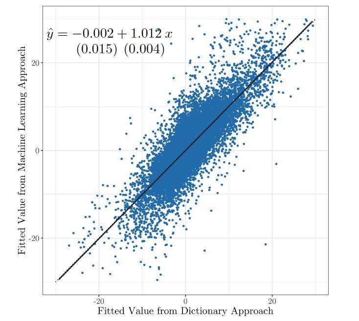
Tremendous Dispersion in U.S. Firm-Level
          Stock Price Reactions to COVID News

                                                                       Reproduced
                                                                       From Davis,
                                                                       Hansen and
                                                                       Seminario-
                                                                       Amez (2021)

                                                                       Classifications of
                                                                       jump days from
IQR is 15 standard                                                     Baker et al. (2021)
deviations greater
than average
IQR in 2019
                 Value-Weighted Mean and Cross-Sectional IQR of U.S. Equity Returns,
                 Daily for 2019 and Large Daily Jumps in February and March 2020.        5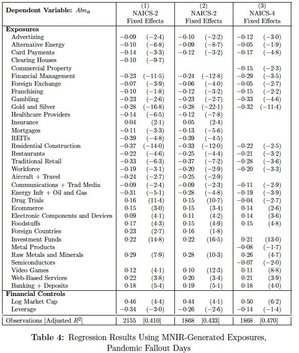
Davis, Hansen & Seminario-Amez (2021)
• Characterize firm-level shock exposures using the “Risk Factors”
  texts in annual 10-K filings.
• Use exposure measures to explain firm-level return reactions to
  market-moving news (daily market-level jumps > |2.5%|)
   –Focus on jumps from late February to end of April (2020).
• Implement and compare two text-analytic approaches:
   –Expert-curated dictionaries (e.g., Tetlock (2007), Loughran-
    McDonald (2011), Baker-Bloom-Davis (2016))
   –Taddy’s (2013) Multinomial Inverse Regression (MNIR), a form
    of supervised machine learning (ML)
• Develop a hybrid approach to uncover new exposures and
  sharpen explanations/interpretations of firm-level returns.
                                                                     6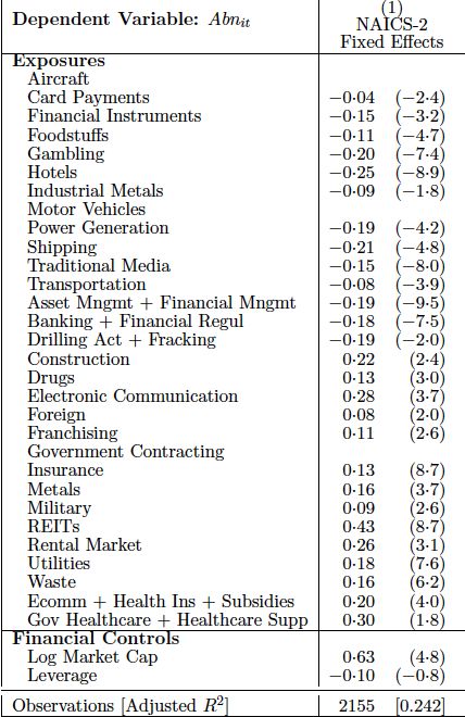
Using the Text in Regulatory Filings to Quantify Firm-
Level Exposures and Characterize Return Drivers

                                                         7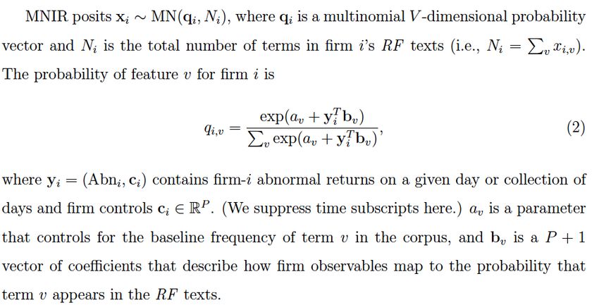
Dictionary Approach
• Dictionaries from Baker et al. (2019), who expand on ones developed by
  BBD (2016) and Davis (2017).
    • 16 dictionaries cover aspects of economic and financial conditions
    • 20 pertain to policy areas.
    • Each dictionary contains terms that effectively define the category.
• In aggregate, the dictionaries contain 244 distinct terms that appear 1.4
  million times (2.4% of the entire RF corpus).
• The RF texts for a given firm contain 28 distinct dictionary terms on average
  (standard deviation of 10) and 642 instances of dictionary terms (standard
  deviation of 620).
• To quantify a firm's exposure to a given category, we identify sentences in
  its RF texts that contain at least one term in the corresponding dictionary.
• After computing the fraction of such sentences in each of the firm’s RF
  texts, we average over years for the firm. This yields 36 firm-level exposure
  values, one for each category.                                            9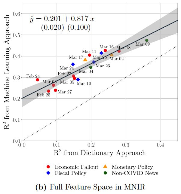
Dictionary Examples
Inflation: {cpi, inflation, gold, silver}
Commodity Markets: {wheat, corn, sugar, cotton, beef, pork,
petroleum, oil, coal, natural gas, biofuel, ethanol, steel, copper,
zinc, tin, platinum, gold, metal, silver, aluminum, lead,
commodity exchange, nymex, mercantile exchange, gas pipeline}
Monetary Policy: {monetary policy, money supply, open market
operations, discount window, quantitative easing, central bank,
federal reserve, the fed, european central bank}
Taxes: {taxes, tax, taxation, taxed, vat, accelerated depreciation,
fiscal cliff, internal revenue service}
Trade Policy: {tariff, dumping, world trade organization, north
american free trade agreement, international trade commission}   10
Firm-Level Return Regressions
(Least Squares)
We fit firm-level return regressions of the form,
Where:
• is the abnormal return of firm i on jump-day t, or its
average abnormal return on a collection of jump dates.
• is firm i’s exposure to category j risks/shocks.
• Leverage and Mcap (market capitalization) are controls.
• is a vector of industry effects (NAICS2 or NAICS4 level).
Under the dictionary approach, captures the effect of
firm i’s exposure to category j on its one-day abnormal equity
return. Fit to data for “jump” days in February and March 2020. 11This table
excerpt
reports our
fitted
dictionary-
based
regression
models for
the 9
pandemic
fallout days
and the 2
monetary
policy
easing days
12Multinomial Inverse Regression Approach, 1
•MNIR treats the RF texts for each firm as a bag-of-words
represented by a V-dimensional vector !" of terms or
``features.’’
• !",$ is the count of term v for firm i, and V = 18,911 is
the number of unique terms in our RF corpus.
•At the firm level, the average number of nonzero
elements in !" is 2,245, with a standard deviation of 891.
13Multinomial Inverse Regression Approach, 2
14Multinomial Inverse Regression Approach, 3
Equation (2) describes a multinomial logistic regression
over V categories, which we fit to 2,155 observations per
jump day, one per firm. Here, we model the probability that
a particular term in V appears in a random draw from the
firm’s RF texts.
We fit (2) using Bayesian regularization methods with a
Gamma-Laplace prior structure on the regression
coefficients. The prior trades off goodness-of-fit and model
complexity, maximizing an information criterion to avoid
over-fitting. See Taddy (2013, 2015) for details.
15Multinomial Inverse Regression Approach, 4
To move from (2) to a forward regression with !"#$ as the
dependent variable, we follow Taddy (2013) and
16How Much Fit Gain from MNIR, and Why?
1718
Comparing Firm-Level Predictions

                                   19
MNIR Captures Much More than Standard Industry Codes
Dependent
variable in
regressions:
1-day firm-level
abnormal
Returns. All
regressions
include
firm-level
financial
controls and
NAICS4 fixed
Effects.
20What Accounts for the Fit?
21Why A Hybrid Approach? •MNIR: impressive predictive performance, but raw results help little to explain/understand what drives the structure of firm-level returns. •By combining MNIR with a semi-automated process for constructing new exposure categories, we: • Sidestep laborious task of constructing expert-curated dictionaries (and lean much less on domain expertise). • Obtain more granular exposure categories & measures. • Fit firm-level returns better than models generated by expert- curated dictionaries. • Obtain straightforward regression results that have much greater interpretive value than MNIR alone. 22
How Our Hybrid Approach Works
Step 1: Select seed terms

                                  23
Step 2: Build term sets corresponding to each seed
Associate each seed with terms in the RF corpus that meet two criteria:
Step 3: Manual pruning of term sets and, in a few
cases, combining term sets
24Exposure Categories for Pandemic
Fallout Dates: Hybrid Approach
2526
Step 4: Compute firm-level exposures

Step 5: Run the same type of regressions as when
using expert-curated dictionaries to generate
firm-level exposures.

                                                   27
How Well Do Our Return Regressions Fit?
Adjusted R-Squared Value in Firm-
Level Abnormal Return Regression
Empirical Nine Pandemic Day after Super
Approach Fallout Days Tuesday Election
Use expert-curated dictionaries and RF
texts to quantify firm-level exposures.
0.33 0.20
Supervised Machine Learning: Forward
regression in MNIR approach of Taddy.
0.50 0.35
Hybrid Approach: Use MNIR to build
limited number of new dictionaries that
0.41 0.24
yield firm-level risk exposure measures
28This table
shows results
of the daily
abnormal
returns
regression fit
to the nine
pandemic
fallout jump
days using
the hybrid
approach.
Apologies for
the small
font.
29This table shows
results of the daily
abnormal returns
regression fit to the
jump day following
the Super Tuesday
primary elections
using the hybrid
approach.
30Summary of Results
1. Bad COVID-19 news lowers returns for firms with high exposures
to travel, traditional retail, aircraft production and energy supply
– directly and via downstream demand linkages – and raises them
for firms with high exposures to healthcare policy, e-commerce,
web services, drug trials and materials that feed into supply
chains for semiconductors, cloud computing & telecom.
2. Monetary and fiscal policy responses strongly impact firm-level
returns as well but differently than pandemic news.
3. Super Tuesday (a huge win for Biden) drove negative returns for
firms with high exposure to hotels, gambling, fracking, and
financial management; and positive returns for firms with high
exposure to healthcare, REITs, property rentals, communications
and construction.
31Summary of Results, 2
4. Despite major methodological differences, dictionary approach
and MNIR yield highly congruent predictions of firm-level returns.
5. By operating on a vastly larger feature space, MNIR outperforms
with respect to goodness-of-fit.
• Our dictionary-based model explains 1/3 of the (huge) firm-
level abnormal return variation on pandemic jump days, while
MNIR explains 1/2.
6. Our hybrid approach outperforms dictionary approach in terms of
model fit and, unlike MNIR, yields readily interpretable results.
7. Our text-based models of firm-level abnormal returns have strong
predictive content for future corporate earnings surprises.
32Text-Based Models Fit to Feb-March 2020 Data Predict
2020 Q3 Earnings Surprises Relative to 2019 Q1 Forecasts
33Concluding Remarks The pandemic-induced return reactions in February-March 2020 that we uncover foretell shifts in the real economy. For example: •Major job losses in the traditional retail sector, employment gains at online shopping and delivery firms, a persistent collapse in air travel, job cuts in aircraft production, numerous bankruptcies among oil and gas companies, a collapse of advertizing revenue in print media, and surging demand for cloud computing. •Evidence that COVID-19 accelerated ongoing shifts to digital services and remote interactions across a host of activities. E.g.., the share of new U.S. patent applications that advance technologies to support video conferencing, telecommuting, remote interactivity, and working from home doubled in the wake of the pandemic. 34
Concluding Remarks, 2
Although often seen as methodological alternatives, our analysis
suggests these expert-curated dictionary methods and supervised
machine learning are complements as much as substitutes.
By combining elements of both, we obtain rich models that (a) fit
better than models based on expert-curated dictionaries, (b) uncover
new, empirically relevant exposure categories missed by the curated
dictionaries and, at the same time, (c) deliver interpretable patterns
in the estimated structure of firm-level returns.
This last feature pushes the supervised ML approach from prediction
to interpretation.

                                                                 35
Extra Slides
36A Standard Asset-Pricing Model
Barro (2006) posits an endowment economy with a representative agent
who has time-separable, isoelastic preferences over consumption. Log
output evolves exogenously as a random walk with drift:
!"($%&' ) = !"($% ) + + + ,%&' + -%&' (3)
where the drift + ≥ 0, ,%&' is i.i.d. normal with mean 0 and variance 0 1 ,
and -%&' picks up low-probability disaster shocks. Barro shows that the
price of a one-period equity claim at t is
454(64')7&('/1)(64')9 : 9
2%' = $% 3 [3 4< + (1 − 3 4< )×E{(1 − B)'46 }] (4)
where ρ is the time preference rate, θ is relative risk aversion, σ is the
standard deviation of the output growth rate absent disasters, E denotes the
expectations operator, p is the disaster probability, and b is the size of the
log output drop when disaster strikes. Agents know the parameters. 37In taking this model to the data, we interpret 17 February as the last date
before disaster strikes and 23 March as the date by which agents fully grasp the
gravity of the disaster. Global and U.S. equity prices fell about 40 percent (51
log points) over this 33-day period. Using (3) and (4), the model-implied
realized equity return over this period is
#$%&'( ,$%&'( 33
!" = !" = - + u3 − v3 , (5)
#)'%*(' ,)'%*(' 365
where v3 is the realized disaster size, and u3 is the realized value of the regular
shock. For any reasonable values of the annual drift (-) and the variability of
regular shocks (9), the first two terms on the right side are tiny compared to v3 .
Thus, the model implies that stock prices should fall nearly one-for-one in
proportion to disaster size. (Given the stochastic process in (3), the rates of
return on one-period and full equity claims are identical.)
38Assessing the Size of the COVID Disaster
Note: The solid lines show U.S. real GDP per capita (from
FRED) plotted in natural log units from 2014 Q1
to 2019 Q4 (solid blue line) and 2020 Q1
to 2020 Q3 (orange line).
The dashed line shows a linear fit to the pre-pandemic
data and its extrapolation to the post-pandemic period.
The maximal gap between the dashed and orange curves
of 11.6 log points which occurs in 2020 Q2.
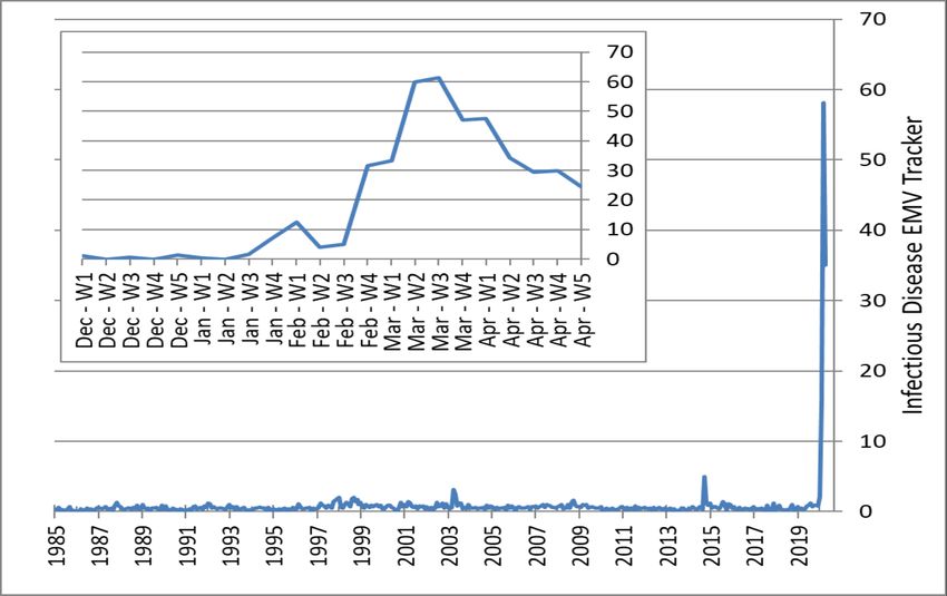
39Infectious Disease EMV Tracker, Weekly and
Monthly Data from 1985 to April 2020
Coronavirus
Weekly from Week 1 of December 2019 (COVID-19)
Bird Flu Swine Flu
SARS MERS/Ebola
(H5N1) (H1N1)
Notes: The Infectious Disease EMV Tracker is computed as the overall Equity Market Volatility Tracker
value multiplied by the share of EMV Articles that contain one or more of the following terms:
epidemic, pandemic, virus, flu, disease, coronavirus, mers, sars, ebola., H5N1, H1N1. See Baker, Bloom,
40
Davis and Kost (2019) and Baker, Bloom, Davis, Kost, Sammon and Viratyosin (2020).Time Path of China Stock Prices and Mobility
from 13 January to 30 April 2020
Note: Stock prices for companies with
equity securities listed on mainland
exchanges only and denominated in
RMB from the CSMAR dataset (China
analog to WRDS). An orange diamond
03/05 marks the first confirmed COVID-19
04/10 death, a green cross marks the first date
02/06
with stringency index value of 70 or
more, and a red dot marks the date on
01/24 which the stringency index first drops
below 70. We linearly interpolate stock
01/31
prices from 24 January to 3 February,
given that mainland China stock markets
were closed from 25 January to 2
February, inclusive.
Source: Davis, Liu and Sheng (2021).
41The Unprecedented Stock Market
Impact of the Coronavirus: China
The same pattern holds for the Hang Seng index (Hong Kong).
Reproduced from “Stock Prices, Lockdowns, and Economic Activity in the Time of
Coronavirus” by Davis, Liu and Sheng (2021). 42Equity Markets Think the Shift to WFH Is a Big Deal
Firms outside ”Critical
Industries” sorted into
quartiles based on the
fraction of workers in
their industry that can
feasibly work from
home.
This chart is from
https://sites.google.co
m/site/lawrencedwsc
hmidt/covid19 and is
based on work by
Schmidt and
Papanikalaou (2020).
4344
Selected Firms with Big Fit Gains on
Pandemic Fallout Days from MNIR45
Clustering of Jump Days Based on MNIR-Fitted Structure
of Returns to Classification Based on Human Readings of
Next-Day Newspaper Explanations for Jumps

                                                          46
An Example of Intra-Industry Differences in Shock Exposures
This chart shows box plots
for the distribution of firm-
level exposures to “Web-
Based Services” for the
indicated industries.
47References
Baker, Scott R., Nick Bloom, and Steven J. Davis, 2016. “Measuring Economic Policy Uncertainty,” Quarterly Journal of Economics.
Baker, Scott R., Nick Bloom, Steven J. Davis and Kyle Kost, 2019. “Policy News and Stock Market Volatility,” NBER WP 25720.
Baker, Scott R., Nick Bloom, Steven J. Davis, Kyle Kost, Marco Sammon and Tasaneeya Viratyosin, 2020. “The Unprecedented Stock
Market Reaction to COVID-19,” Review of Asset Pricing Studies,10, no. 4.
Baker, Scott R., Nick Bloom, Steven J. Davis, and Marco Sammon and Tasaneeya Viratyosin, 2021. “What Triggers Stock Market Jumps?”
NBER Working Paper 28687.
Barrero, Jose Maria, Nicholas Bloom and Steven J. Davis, 2020. “COVID-19 Is Also a Reallocation Shock,” Brookings Papers on
Economic Activity, Summer.
Barrero, Jose Maria, Nicholas Bloom and Steven J. Davis, 2021a. “Why Working from Home Will Stick,” NBER Working Paper 28731.
Barrero, Jose Maria, Nicholas Bloom, Steven J. Davis and Brent Meyer, 2021b. “COVID-19 Is a Persistent Reallocation Shock,” AEA
Papers & Proceedings, May.
Barro, Robert J., 2006. “Rare disasters and asset markets in the twentieth century,” Quarterly Journal of Economics, 121, no. 3.
Davis, Steven J. 2017. “Regularity Complexity and Policy Uncertainty: Headwinds of Our Own Making,” working paper.
Davis, Steven J., Stephen Hansen and Cristhian Seminario-Amez, 2020. “Firm-Level Risk Exposures and Stock Price Reactions to
COVID-19,” NBER Working Paper 27867.
Davis, Steven J., Dingqian Liu and Xuguang Simon Sheng, 2021. “Stock Prices, Lockdowns, and Economic Activity in the Time of
Coronavirus,” NBER Working Paper 28320.
Lougran T. and B. Mcdonald, 2011. “When Is a Liability Not a Liability? Textual Analysis, Dictionaries, and 10-Ks,” Journal of Finance,
66, no. 1.
Papanikolaou, Dimitris and Lawrence D.W. Schmidt, 2020. “Working Remotely and the Supply-Side Impact of COVID-19,” NBER
Working Paper 27330.
Taddy, Matt, 2013. “Multinomial Inverse Regression for Text Analysis,” Journal of the American Statistical Association, 1108, no 503.
Taddy, Matt, 2015. “Distributed Multinomial Regression,” Annals of Statistics, 9, no. 3, 1394-1414.
Tetlock, Paul C., 2007. “Giving Content to Investor Sentiment: The Role of Media in the Stock Market,” Journal of Finance, 62. no. 3.You can also read


