Projektbericht - Population projection for Germany 2015-2050 on grid level (RWI-GEO-GRID-POP-Forecast) - RWI Essen

Projektbericht

Philipp Breidenbach
 Matthias Kaeding
 Sandra Schaffner

 FDZ Data description
 Population projection for Germany 2015–2050
 on grid level (RWI-GEO-GRID-POP-Forecast)

Impressum

Herausgeber:
RWI – Leibniz-Institut für Wirtschaftsforschung
Hohenzollernstraße 1–3 | 45128 Essen, Germany

Postanschrift:
Postfach 10 30 54 | 45030 Essen, Germany

Fon: +49 201–81 49-0 | E-Mail: rwi@rwi-essen.de
www.rwi-essen.de

Vorstand
Prof. Dr. Christoph M. Schmidt (Präsident)
Prof. Dr. Thomas K. Bauer (Vizepräsident)
Dr. Stefan Rumpf

© RWI 2017
Der Nachdruck, auch auszugsweise, ist nur mit Genehmigung des RWI gestattet.

RWI Datenbeschreibung
Schriftleitung: Prof. Dr. Christoph M. Schmidt
Gestaltung: Daniela Schwindt, Magdalena Franke, Claudia Lohkamp

FDZ Data description
Population projection for Germany 2015–2050 on grid level
(RWI-GEO-GRID-POP-Forecast)

Autoren
Dr. Philipp Breidenbach, Matthias Kaeding und Dr. Sandra Schaffner

Projektbericht

 RWI – Leibniz-Institut für Wirtschaftsforschung

 FDZ Data description

Population projection for Germany 2015–2050
 on grid level (RWI-GEO-GRID-POP-Forecast)

RWI-GEO-GRID-POP-Forecast

List of contents
List of table and figures ...................................................................................................................4
0 Abstract ...........................................................................................................................5
1 Introduction .....................................................................................................................6
2 Data .................................................................................................................................8
3 Results ........................................................................................................................... 12
4 Scopes and Limitations .................................................................................................. 16
5 Data Availability .............................................................................................................. 17
6 References ..................................................................................................................... 18

 3

RWI

List of table and figures

Figure 1 Populated grids in Germany................................................................................................7
Figure 2 Annual death rate and arising life expectancy ................................................................... 9
Figure 3 Net migration flows .......................................................................................................... 10
Figure 4 Birth rates on county level .................................................................................................11
Figure 5 Probability of childbearing ................................................................................................11
Figure 6 Projected Population 2015 to 2050.................................................................................... 12
Figure 7 Mean age of the projected Population 2015 to 2050 .......................................................... 13
Figure 8 Stylized size of age cohorts ............................................................................................... 13
Figure 9 Regional variation of the mean age .................................................................................. 14
Figure 10 Old-age dependency ratio for Berlin ............................................................................... 14

Table 1 Population changes on municipality level ........................................................................... 15

4

RWI-GEO-GRID-POP-Forecast

0 Abstract
 Existing nationwide population projections focus on highly aggregated spatial units. The most re-
gionalized nationwide study is provided by the German Federal Institute for Building, Urban Affairs
and Spatial Research (BBSR) and predicts population on county level up to 2035 (BBSR 2015). Pro-
jections of the German Federal Statistical Office – marking the benchmark approach for German
population projections – are constraint to agglomerated projections for entire Germany or for federal
states, provided by the state offices. Existing small scaled data e.g. the RWI-GEO-GRID impressively
reveal the high heterogeneity of local socioeconomic traits within commonly applied county- or mu-
nicipality-data. Based on these existing population data on the grid level (offering a resolution of
1×1km-grids), the presented RWI-GEO-GRID-POP-Forecast provides a population projection up to
2050. The applied methodological concept strongly follows the approach of the German Federal
Statistical Office and the agglomerated results are in line with this projection. This article gives an
overview on the provided dataset, the applied methods, some basic results and the access to the
data for scientific purposes.

 5

RWI

1 Introduction
 The demographic structure in Germany changes due to low fertility rates and increased life expec-
tancy. Focusing on the natural development, Germany faces a shrinking and aging population. Ex-
pected migration flows will weaken these effects but it is not predicted to turn around. These devel-
opments are recorded by the German Federal Statistical Office in their German-wide projection
(Destatis 2015a) for the years up to 2060. Depending on underlying assumptions, the population will
shrink to about 70 million people in 2060 and the share of people over 65 years will increase from
21 % to about 32 %. These expected developments have substantial effects for various major fields
of economic policy. Public finances as well as the labor market and the demand for public services
and infrastructure are highly affected by the decrease and aging of the population.
 By definition, these German-wide projections disregard the wide variety of demographic change
on lower regional levels as these projections are only available on administrative levels like Federal
States or county. The demographic structure on lower levels is quite heterogeneous, which implies
that Federal State and country are too large to capture regional heterogeneity adequately. Especially
for child or elderly-care services, supply of medical care or local transport services areas below the
county level serve the right delineation to describe local needs. Up to now, there is a lack of such
data which offer a nationwide consistent demographic projection based on reliable data sources for
small scaled areas.
 To fulfill the need for such data, the Research Data Centre Ruhr at RWI (FDZ Ruhr) has developed
a demographic projection based on grid data. The grids are defined as 1×1 kilometer squares which
cover Germany in spatially equal units. In comparison to common administrative data, synthetic grid
data offer major advantages: (1) Grid data can be easily transformed into administrative regions. (2)
Spatial grids are time-independent, unlike e.g., German counties or zip codes. (3) Grid data can be
efficiently stored, analyzed and linked with other data types (4) The grids offer a high spatial reso-
lution to uncover heterogeneities in less dense populated areas, despite German counties or zip
code areas.
 This report summarizes the underlying method of this grid-based population projection for Ger-
many from 2015 to 2050, based on main assumptions from Destatis (2015a). The assumptions con-
sider birth probabilities, life-expectancy, net migration and expected changes in fertility, mortality
and migration. The projection is based on grid-level population data, the RWI-GEO-GRID (RWI/mi-
crom 2017), described in Budde/Eilers (2014). The grid level projection is comparable to the official
in its aggregation but it accounts for the substantial spatial variation.
 The paper is organized as follows. Section 2 gives a detailed overview of the data, the applied
methodology and the underlying assumptions. The results in section 3 show that our projection is in
line with existing nationwide projections of the Federal Statistical Office and give some insights into
the data. Section 4 sums up and gives information on the data availability.

6

RWI-GEO-GRID-POP-Forecast

Figure 1
Populated grids in Germany

Source: RWI/ microm (2017).

 7

RWI

2 Data
 The population projection is based on population data on the 1km² grid level from the RWI-GEO-
GRID, a dataset containing population information disaggregated by gender and age. Age is divided
into 17 age intervals 1. These data are available for 216 831 populated 1km² grid-cells 2 as defined
under the ETRS89 Lambert Azimuthal Equal-Area projection coordinate reference system (Annoni
2003). Figure 1 presents the distribution of populated grid cells, 39.66% of all German grid cells are
not populated.
 For forecasting purposes, the underlying population data presented in age intervals are trans-
formed into a population cohort for every age-year. As the last age interval (75, infinity) has no
information on the maximum age in this group, the age distribution is treated as truncated at 100
 
years. The RWI-GEO-GRID contains the number of people , ,2015 ,in 2015 by sex [s] for age interval
 
[i] in grid g=1,…, 216 831. However, the number of inhabitants , ,2015 for each age [a] is needed.
Therefore, a meaningful transformation of the given intervals into age-years is applied. Note that
 
 , ,2015 = ∑ , ,2015 .
 Define
 
 , ,2015
 , ,2015, ∶= ,
 , ,2015

 than
 
 , ,2015 = , ,2015, , ,2015 ,
 so that the population data can be transformed into age-years given an estimate for , ,2015, .
This fraction is taken from administrative county-level data which are available in age-year resolu-
tion up to the age of 85. The estimator for , ,2015, is given by the county-specific fraction
 , ,2015, 
 
 , ,2015
 of the county in which the majority of the area of the grid cell g is located. This method assumes
that the real fraction of each age-year within an age-interval is fix on the county level. For ages
above 85, German wide fractions of ages are used for all grid cells, as no population numbers are
available in age-year resolution for counties.
 This prepared database offers a good starting point for the projection algorithms. Basically two
algorithms are at work, the main one projects the non-newborn population in each year (i.e. age >
0), the other one projects the newborns for each year which can naturally not be derived by the
lower age-year in the past year (t-1). The non-newborn population N is estimated as
 −1 −1 
 , , = , , −1 − , , −1 + , , 

 for each grid g, sex s and year t=2016,…,2050 at the age-years a=1,…,100. D denotes the number of
deceased persons and M denotes net migration. For notational clarity, no distinction between esti-
mated or known entities is made. The number of deceased people is calculated by the life-expec-
tancy and its expected development over time. The migration in each age group comes from the
expected total migration for each year. These assumptions are described in the following para-
graphs.

1 i=[0,2],…,[6,9],[10,14],[15,17],[18,19],[20,24],[25,29],…,[65,74],[75,infinity),
2 About 40% of the grid cells covering Germany are not populated.

8

RWI-GEO-GRID-POP-Forecast

Figure 2
Annual death rate and arising life expectancy
Death rate by sex and age-year

Source: Estimated from the Lee-Carter model (1992). Note: The reported death rates imply an increasing life expectancy for
women from about 83.33 (men: 77.69) in 2015 to 86.93 (men: 82.80) in 2050.

 Life expectancy: It is assumed that life expectancy increases over time. The probability of death is
predicted using the popular Lee-Carter (1992) method, which can be viewed as the benchmark
method. The following model is assumed for the probability of death q, conditional on surviving up
to the age a -1:
 E[log( , , )] = , + , * , .
 The parameter , represents the mean life-expectancy of gender s and age-year a at time t, , 
represents the overall level of mortality at time t, for gender s which is adjusted by the gender and
age-group specific coefficient , . For , , a random walk with drift is assumed. The German-
wide death rates are projected to fall for each age-year by sex for 2015 and 2050 (Figure 2). The
underlying parameters are estimated using observed German-wide death rates from Destatis
(2015c). In the years 2015 to 2050, female life expectancy is projected to increase from 83.33 to 86.93
years, male life expectancy is projected to increase from 77.69 to 82.80 years. This trend is also
observed in the calculated death probabilities for the projected period. The death rate for each age-
year decreases. This decrease is the largest for young and middle-aged males. Focusing on the
highest age group, the decrease of death probability from 2015 to 2050 is rather weak. The under-
lying parameters are estimated using observed German-wide death rates from Destatis (2015c). Es-
timation is carried out using the R-package forecast (Hyndman et al. 2014).
 Specific death rates on lower regional levels are not used in the projection. These variations in
death rates are assumed to stem from worse health conditions in (former) employment and former
differences in the medical care system. We assume that these differences in death rates will vanish
over time.
 Net migration: Net migration is defined as the difference between immigrants and emigrants. The
net migration was driven by several trends during the last years (Figure 3). Before the start of the
financial crisis in 2008, Germany was characterized by very low or even negative net migration.
Afterwards, the rather strong German recovery compared to other European countries and the large
immigration flows due to the refugee crisis turned the net migration highly positive. Based on these
very different developments expectations on future migration are hard to make. Our projection as-
sumes a sequential decrease of net migration from the observed value of 1.13 million people in 2015
to 150 000 in 2020 (Figure 3). This value is approximated from the median net-migration inflow
before the migration wave from 2001 to 2015 (142 645). In line with the German-wide projection by
the German Federal Statistical Office, the net migration stays constant afterwards. Our long-term
migration is right in between the two scenarios which Destatis (2015a) applies (migration surplus of
100 000 or 200 000 per year). However, the short-run projection is much higher since the projection
of Destatis (2015a) was made just in the beginning the big refugee inflow. The age structure of the

 9

RWI

migrants is assumed to be constant over time and is derived from Destatis (2015a). Since there is no
information on future regional distribution of the migration, the regional migration surpluses are
based on the existing population. The net migration inflow is separated to each grid by its share of
the total population.
Figure 3
Net migration flows
Historical data up to 2013, assumed data up to 2050. In 1 000 persons.

Source: Destatis (2016a) for historical data – own assumptions for future values.

 Future intra-German flows are ignored in this projection since there is no reliable estimation on
the extent and direction of these future flows. Since the underlying movements on such small spatial
levels are a result of wages, unemployment, housing prices and connectivity and there are no long-
term small area predictions on these parameters, a resilient projection cannot cover these parame-
ters. Constant flow parameters can instead be added by users (e.g. assuming that urbanization
trends relocate a share of a certain population group from each rural to each urban area). The
projection can highlight the basic natural development in terms of an aging and mostly decreasing
population which can be compensated by good local competitiveness or be accelerated by a bad
policy.
 The projected number of newborns is based on the female population aged between 16 and 49,
which is assumed to be the period of birth-giving age:
 49
 0 
 , , = ∗ � , , ∗ , ,
 =16
 where fraction s 3 is the mean fraction of births of sex s taken from the years 1980 to 2015. The age-
specific fertility rate p of women at age a at time t and grid g must be simulated.
 Age-specific fertility rates: It is assumed that fertility rates vary over time and space. Regional
differences are accounted for by using county-specific birth rates, obtained from Destatis (2015b).
These differences in fertility rates are expected to be persistent. Figure 4 illustrates the variation for
Germany on county-level showing higher fertility rates in former Eastern German states and lower
rates on average in western parts. The rate varies from 1.07 children per women to 1.79.

3The mean fractions of births are: fractionfemale: 48.6633% and fractionmale: 51.3367%.

10

RWI-GEO-GRID-POP-Forecast

Figure 4
Birth rates on county level
Expected number of birth per woman.

Source: Computation based on Destatis (2015b).

 Furthermore, it is assumed that the age of women with the highest probability of giving birth shifts
from 31 in the year 2015 to 33 in the year 2028 and remains on this level afterwards. We assume that
the number of births per woman increases from 1.5 in the year 2015 sequentially to 1.6 in the year
2028 and stays constant in the years 2029 to 2050. This assumption is in line with Destatis (2015a).
Figure 5 shows a sample of resulting fertility rates for each age-year of women between 16 and 49
for 2015 and 2050.
Figure 5
Probability of childbearing
By age of women for 2015 and 2050.

Source: Destatis (2015b) – own assumptions for future values.

 11

RWI

3 Results
 The result section is intersected in two main strands. Before some stylized facts and maps are
presented, the long-term trends in the age structure of the aggregated German projection results
are compared to the results of Destatis (2015a). As the Destatis (2015a) projections can be seen as
the gold-standard of German population projections, a similarity can raise the credibility. Destatis
(2015a) computes different scenarios, we use “Variant 2: Continued trend based on higher immigra-
tion” as reference: This variant assumes the highest level of net migration, matching the observed
net migration in the most recent years somewhat better than the other variants.
 On the aggregated level, the German population is decreasing in size, as more people are dying
than being born or migrate to Germany. Figure 6 compares the total population by sex for each
projected year until 2050. The trends shown in both projections are similar, beginning with a trend
of increasing population (due to migration) there is a turnaround around the years 2020/2025 with
an ongoing decrease of population. While our projection starts with a slightly lower number of in-
habitants, the two projections intersect quickly around 2017 and the RWI-data project a higher pop-
ulation afterwards. While our data indicate 0.7% less population in the underlying data, we project
2.6% more inhabitants for 2050.
 These differences stem from different assumptions on migration. The reference scenario of Destatis
(2015a) assumes a lower level of migration for the years up to 2020. We assume a net migration
surplus of 3.87 million in the years 2015 until 2020, resulting in 1.62 million more migrants until
2020 compared to Destatis (2015a). Furthermore, we project a slightly lower level of migration for
the ongoing years afterwards (150 000 migrants per year compared to 200 000). Due to recent mi-
gration waves which could not be taken into account by Destatis (2015a) as their figures were defined
before the migration accelerated noticeably, our assumption seems to be plausible.
Figure 6
Projected Population 2015 to 2050
Comparison of Destatis (2015) and RWI-projection by sex in million people.

Source: Computation based on Destatis (2015b).

 Furthermore, our data slightly differ in the underlying age structure (Figure 7). In terms of mean
age, the population of our data is slightly younger (about three months). The difference increases
until the end of the projection period to about seven months. This development also stems from the
different assumption on migration. In contrast to the existing aging in society, the age structure of
migrants is assumed to be constant over time. As migrants gain a higher weight in our projections
(due to higher inflows), the lower mean age can be explained.

12

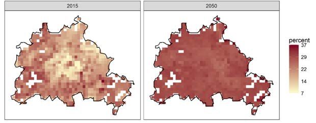
RWI-GEO-GRID-POP-Forecast

Figure 7
Mean age of the projected Population 2015 to 2050
Comparison of Destatis (2015a) and RWI-projection by sex

Source: Destatis (2015a) – own assumptions for future values

 Since our projection shows quite sophisticating results compared to Destatis (2015a), we proceed
with some further summarizing statistics especially on the spatial variation of our results. Figure 8
shows stylized developments of the age cohorts over the projected years. The baby boomer aged
about 50 in 2020 mark a peak of the distribution and represent the largest cohort of the population.
Their child-generation (aged about 25 to 35 in 2020) mark a local maximum as well as the pre-war
generation aged about 75 in 2020. Due to higher life-expectancy, the female distribution has a
stronger peak in this higher age. For the case of females, the baby-boomer generation will remain
the largest cohort in the 2050 distribution. For the male distribution, the lower life expectancy scales
down this generation earlier and the generation aged 20 to 30 today will become the largest popu-
lation. Due to the expected long-term fertility rate of 1.6, the following generations will remain
smaller than their parental generations.
Figure 8
Stylized size of age cohorts
For selected projected years by sex.

Source: Own assumptions for future values.

 13

RWI

 However, the strongest benefits of our data can be regarded in the detailed observation of spatial
differences. Figure 9 shows the mean age for Germany in 2015, 2033 and 2050. There is a consider-
ably difference in age structure between East and West Germany; the mean age is around two years
higher in East Germany. For the year 2033, this stays approximately constant while the mean age is
shifted upwards.
Figure 9
Regional variation of the mean age
Interpolated values based on grid level.

Source: Computation based on own projections. Note: Interpolation for 216.831 grids is done using a generalized additive
model, see Wood (2006).

 While the information presented yet can also be extracted from existing data especially on the
county level (BBSR 2015), Figure 10 gives an impression on the detailed information provided by our
data. The map shows the old-age dependency ratio for Berlin in 2015 and 2050. At the starting point
in 2015, the ratio varies from 7% to about 35 % derived by a few exceptions. In 2050, the mean ratio
is significantly higher and converges between the grids.4
Figure 10
Old-age dependency ratio for Berlin
In percent for 2015 and 2050.

Source: Computation based on own projections.

 Some information on the municipality-developments are listed in Table 1. Those ten municipalities
with the highest population gains and losses are shown as well as those with the strongest devel-
opments in the old-age dependency ratio. Municipalities with less than 5 000 inhabitants (in 2015)
are ignored since their gains and losses in percentage are prone to be driven by outliers. The data
show substantial changes due to natural demographic changes. The municipalities with the largest
loss loose more than 25% percent of their population. Eastern German municipalities dominate this
snapshot. Contrary, the municipalities with the highest gains of inhabitants are dominated by uni-
versities.

4 Especially for the case of Berlin, the ignored inner-German migration will change the results. However, such inflows will
intensify the small-scaled variation, making such grid data more important.

14

RWI-GEO-GRID-POP-Forecast

Table 1
Population changes on municipality level
Municipalities with largest losses and gains.
Municipality Inhabitants Inhabitants Change
 2015 2050 (in percent)
Guben 17 304 12 370 -28.5
Hoyerswerda 34 624 24 872 -28.2
Klingenthal 8 905 6 404 -28.1
Bad Füssing 6 789 4 901 -27.8
Grömitz 6 469 4 692 -27.5

Tübingen 85 212 103 208 21.1
Marburg 73 873 88 796 20.2
Gießen 77 966 92 828 19.1
Heidelberg 156 514 180 747 15.5
Hallbergmoos 10 073 11 571 14.9
Source: Computation based on own projections.

 15

RWI

4 Scopes and Limitations
 This article presents the RWI-GEO-GRID-POP-Projection – a population projection up to 2050 based
on 1×1km-grid data. This is the first nationwide projection considering spatial heterogeneity on such
a detailed level. The data are based on the RWI-GEO-GRID which contain population information for
detailed age groups. Projections are mostly in line with the German-wide projection from the Ger-
man Federal Statistical Office (Destatis 2015a). Fertility rates are regionalized as we assume that
there are persistent regional differences in the probability of having children. We do not assume
that differences in life expectancy are persistent over time as they massively reflect former employ-
ment which were harmful to health and former different medical services which are not assumed to
be persistent.
 As the basic factors of the projection by the Federal Statistical Office were defined before the mas-
sive migration wave beginning in 2015, we have increased the short-term migration for the years
up to 2020. In contrast to German-wide projections, we have to deal with the regional distribution
of migrants and intra-German flows.
 We assume that migrants distribute along the distribution of the total population. Future intra-
German flows are ignored in this projection since there is no reliable estimation on the extent and
direction of these future flows. Since the underlying movements on such small spatial levels are a
result of wages, unemployment, housing prices and connectivity and there are no long-term small
area predictions on these parameters, a resilient projection cannot cover these parameters. Constant
flow parameters can instead be added by users (e.g. assuming that urbanization trends relocate a
share of a certain population group from each rural to each urban area).
 Nevertheless, the projection can give a solid base on natural population development until 2050.
Comparing our results with the German-wide projection offer sophisticating results. Differences in
predicted total population and mean age can be explained by different assumptions on migration
while our migration assumptions have taken recent migrant waves into account.
 Our results suggest an aging society and shrinking population in Germany. Migration can slow
down (but not stop) this development. These trends differ substantially over the regions. A snapshot
on remarkable developments on municipality level show decreases up to 29% on the one side and
a gain in population of 21% from 2015 to 2050 on the other side.
 The dataset can be merged with basically all datasets which contain precise geographical infor-
mation (longitude/latitude or grid information). These data – as well as other grid information e.g.
provided by the RWI-GEO-GRID – can revalue existing datasets when they are merged as so-called
context data. Moreover the data can be aggregated to higher ordered regional entities. We have
good experience with aggregation on zip code or municipality level. The data also promise new
insights into demographic development on the municipality level since it is the first German wide
projection on this level.
 Regarding the research potential, these data allow research directly focused on demographic de-
velopments e.g. the provision and location of local infrastructures should be planned regarding the
local demographic trends.

16

RWI-GEO-GRID-POP-Forecast

5 Data Availability
 The data are available as a scientific use file (SUF) for scientific, non-commercial, research. The
data is stored efficiently using a wide format, where the rows are given by the combination of grid
cell, sex and age and the columns are the forecasted population numbers. 5 The data can be obtained
as a Stata® dataset (dta), R dataset (rds), Excel (xlsx) or csv. Data access requires a signed data use
agreement. Only researchers of scientific institutions are eligible to apply for data access to the SUF.
The SUF can be used at the workplace of the users. Upon request, we can provide snapshots of the
data or data on higher aggregated regional levels as public use file for non-scientists.
 Data access is provided by the Research Data Centre Ruhr at the RWI – Leibniz-Institute for Eco-
nomic Research (FDZ Ruhr). Data access can be applied for online at http://fdz.rwi-essen.de/appli-
cation.html. The application form includes a brief description and title of the project, cooperation,
department, expected duration of data usage as well as further participants in the project.

5 See http://fdz.rwi-essen.de/doi-detail/id-107807popforecastsufv1.html for meta data registered with the DOI. The meta data as
related publications are updated regularly.

 17

RWI

6 References
Annoni (2003). European Reference Grids. Proposal for a European Grid System. Workshop
Proceedings and Recommendations. EUR Report 21494 EN.
BBSR (2015). Die Raumordnungsprognose 2035 nach dem Zensus. In BBSR-Analysen Kompakt
05/2015.
Budde, R., & Eilers, L. (2014): Sozioökonomische Daten auf Rasterebene: Datenbeschreibung der
microm-Rasterdaten (No. 77). RWI Materialien.
Destatis (2015a). Bevölkerung Deutschlands bis 2060. 13. koordinierte
Bevölkerungsvorausberechnung. Statistisches Bundesamt: Wiesbaden.
Destatis (2015b). Geburten: Lebendgeborene nach Geschlecht, Nationalität und Alter der Mütter.
Destatis (2015c). Sterbetafel (Periodensterbetafel): Deutschland, Jahre, Geschlecht, Vollendetes Alter.
Destatis (2016a). Wanderungen: Wanderungen zwischen Deutschland und dem Ausland 1991 bis
2015.
FDZ Ruhr am RWI (2017): Population Forecast. RWI-GEO-GRID. Version: 1. RWI – Leibniz-Institut für
Wirtschaftsforschung. Datensatz. http://doi.org/10.7807/pop:forecast:suf:v1
Hyndman, R. J. & Booth, H. & Tickle, Leonie & Maindonald, John (2014): demography: Forecasting
mortality, fertility, migration and population data. R package version 1.18.
Lee, R. D., & Carter, L. R. (1992). Modeling and forecasting US mortality. Journal of the American
statistical association, 87(419), 659-671.
RWI; microm (2017). Socio-economic data on grid level (Wave 5). Population by age and gender.
RWI-GEO-GRID. Version: 1. RWI – Leibniz-Institut für Wirtschaftsforschung. Datensatz.
http://doi.org/10.7807/microm:einwGeAl:V5
Wood, S. N. (2006). Generalized Adaptive Models: An Introduction with R. Chapman and Hall/CRC.

18