STQ-Nets: Unifying Network Binarization and Structured Pruning - BMVC 2020
←
→
Page content transcription
If your browser does not render page correctly, please read the page content below
MUNAGALA ET AL.: UNIFYING BINARIZATION AND PRUNING                                               1

STQ-Nets: Unifying Network Binarization
and Structured Pruning
Sri Aurobindo Munagala1                             1
                                                        Center for Visual Information
s.munagala@research.iiit.ac.in                          Technology
Ameya Prabhu2                                           Kohli Center on Intelligent Systems
ameya@robots.ox.ac.uk                                   IIIT-Hyderabad, India
                                                    2
Anoop Namboodiri1                                       Department of Engineering
anoop@iiit.ac.in                                        University of Oxford, UK

                                             Abstract
          We discuss a formulation for network compression combining two major paradigms:
      binarization and pruning. Past works on network binarization have demonstrated that
      networks are robust to the removal of activation/weight magnitude information, and can
      perform comparably to full-precision networks with signs alone. Pruning focuses on
      generating efficient and sparse networks. Both compression paradigms aid deployment
      in portable settings, where storage, compute and power are limited.
          We argue that these paradigms are complementary, and can be combined to offer high
      levels of compression and speedup without any significant accuracy loss. Intuitively,
      weights/activations closer to zero have higher binarization error making them good can-
      didates for pruning. Our proposed formulation incorporates speedups from binary con-
      volution algorithms through structured pruning, enabling the removal of pruned parts of
      the network entirely post-training, beating previous works attempting the same by a sig-
      nificant margin. Overall, our method brings up to 89x layer-wise compression over the
      corresponding full-precision networks – achieving only 0.33% loss on CIFAR-10 with
      ResNet-18 with a 40% PFR (Prune Factor Ratio for filters), and 0.3% on ImageNet with
      ResNet-18 with a 19% PFR.

1    Introduction
Network binarization is a powerful compression paradigm, which quantizes full-precision
32-bit weights and activations to a 1-bit {-1,+1} scale. Binary networks retain information
exclusively related to spikes (i.e. important signal or not), discarding information about
magnitude of spikes (how important) in weights and activations of deep networks preserves
their performance to a surprising extent. Early works focused on finding suitable binary
approximations for training binary networks [8, 9, 29, 31], while recent works [3, 18, 19, 24]
focused on enhancing informational flow to adapt recent architectures with binary networks.
    In this work, we explore the direction of investigating the limits of binary network com-
pression by introducing pruning, while preserving accuracies. This is difficult to achieve
compared to full-precision networks, since binary networks have far fewer redundancies ow-
ing to the reduction from 32 bits to a single bit for weights. Intuitively, weights/activations
closer to zero have higher binarization error making them good candidates for pruning, as
removing weights with high binarization error has little impact on the network. Hence, our
primary idea is that structured filter-level pruning can work in tandem with binarization to
2 MUNAGALA ET AL.: UNIFYING BINARIZATION AND PRUNING
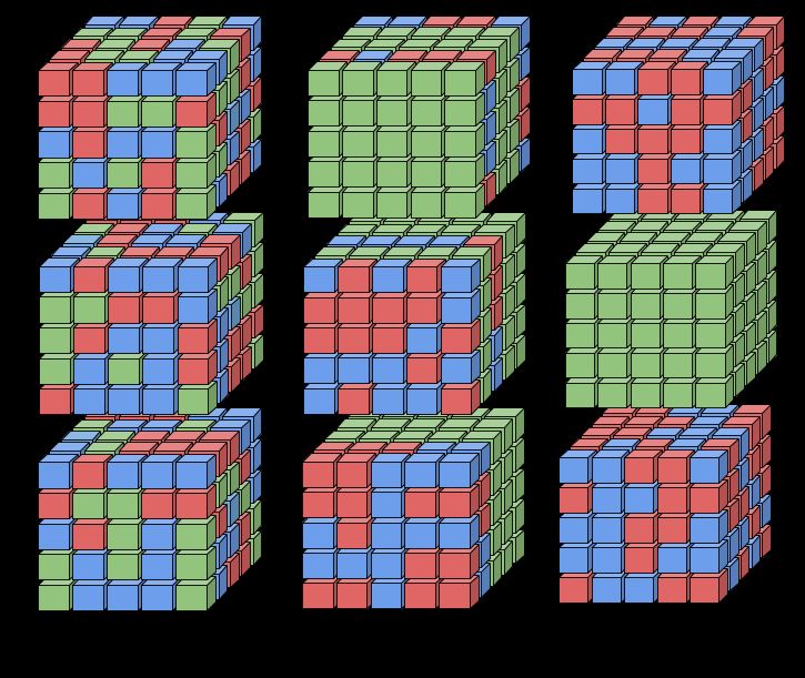
Figure 1: A comparison between (a) unstructured ternary weights, (b) STQ-B weights (c) STQ-A
weights, with each 5x5 cube representing a filter, green denoting a value of 0, and red/blue denoting
{-1,+1}. In (a), 0s are interspersed with {+1,-1} values, making it difficult to make use of fast binary
convolution algorithms. In (b), filters with certain channels/filters zeroed out, creating 3 binary chan-
nels. In (c), entire green({0}) filters can be removed entirely from the network. Thus, (b) and (c) are
compatible with fast binary convolution algorithms with higher overall speedups.
result in extremely compressed binary networks without significant loss. There has been
very limited exploration this direction [35, 36].
Past works on ternary representations [1, 7, 14, 33] generally quantize convolution layer
weights to {-1, 0, +1}; these unstructured weight matrices (i.e. with 0s interspersed with bi-
nary values in an unstructured manner), even with binary activations, are incompatible with
fast binary convolution algorithms and cannot leverage those speedups on any general pur-
pose CPU. In contrast, our structured ternary representations are constrained to the channel
level: individual channels are either fully binary ({-1, +1}, which are retained) or fully 0
(which are removed). We illustrate this in Figure 1. This structured pruning enables easy
removal of fully zero parts of the network, leading to high speedups with binary convolution
algorithms (based on XNOR-Popcount operations) at inference time.
We explore two approaches towards learning these structured ternary representation:
adapting 0 weights after learning a binary network, and adapting binary weights after fix-
ing 0 weights through masks. In the former (STQ-A), we train the network with binary
weights {-1,+1} while imposing a sparsity regularization on scaling values attached to fil-
ters. We prune away filters with low scaling factors after a round of training, and re-train
the network. In the second approach (STQ-B), we initialize filter masks before training the
network to zero them, and then train to learn weights of the remaining binary weights. Our
technique performs well across a wide range of settings: weight-binarized and weight-and-
input-binarized networks, different binarization and pruning algorithm combinations, across
various datasets and architectures. We hope that our work encourages exploration in the
direction of further compression on binary networks.MUNAGALA ET AL.: UNIFYING BINARIZATION AND PRUNING 3
2 Related Works
Binarization and pruning have been extensively studied directions for network compression.
We refer the reader to the surveys by Qin et al. [28] and Blalock et al. [4] for detailed review
of these areas.
Binary Networks: Binarization methods learn efficient and accurate networks with bi-
nary {-1,+1} weights and/or activations. Iniitial explorations achieved near state-of-the-art
performance on weight binarization, on MNIST with EBP [6, 31], CIFAR-10 with Bina-
ryConnect [8] and ImageNet with BWN [29]. This motivated work in full-binarization (bi-
narizing both weights and activations), with BinaryNet [9] demonstrating performance on
CIFAR-10 by approximating using a straight-through estimator [2]. XNOR-Net [29] im-
proved on this to achieve high performance on ImageNet by introducing a scaling factor
for filters. [5, 37] trained these scaling factors as parameters, among other tweaks [3, 32]
to improve binary network training. Real-to-Bin [24] further introduced a novel distilla-
tion loss, reaching to within 3-5% of accuracy with ResNet-18 on ImageNet. Several works
have attempted architectural tweaks for high overall performance as well. Bi-Real Net [19]
avoided binarizing downsample convolutions, and Prabhu et al. [26] designed an algorithm
to automatically determine layers to binarize. Works like ABC-Net [18], Group-Net [42] and
binary ensembles [41] used multiple parallel binary layers to improve accuracies while us-
ing higher computational expense. Our work utilizes and builds on these methods to achieve
further compression and speedups, which has seen little previous exploration.
Ternary Quantization: Ternary quantization approaches quantize network weights to
{-1, 0, +1}. TBN, TTQ[7, 14] propose approaches towards effective ternary quantization for
weights, performing comparably to full-precision counterparts. INQ [38] presents an effec-
tive low-bit quantization method and also combines their approach with pruning. TBN [33]
and GXNOR-Net [10] provide methods to gain high computational speedups using ternary-
binary and ternary-ternary inputs/weights respectively. Ternarized-weight networks, how-
ever, are unstructured, with the 0 values interspersed with {-1,+1} weights and thus requir-
ing 2 bits to store each weight. Our work performs structured ternarization to weights where
0 values occur as whole channels, which can simply be removed from the network - also
allowing full computational speedups available to binary networks.
Pruning: Pruning techniques involve sparsifying networks by removing parameters ef-
ficiently without loss to accuracy, and can be generally categorized into structured versus
unstructured methods. Unstructured pruning algorithms such as [11, 20, 40] remove indi-
vidual weights interspersed through the layer, which is not beneficial towards gaining high
computational speedups. Structured pruning techniques involve constraints that allow the
pruned networks to directly take advantage of faster computation without requiring addi-
tional calculation algorithms or specialized hardware. Of these, filter-level pruning methods
aim to find and remove entire filters through metrics such as effect on final output [15], statis-
tics from the subsequent layer [23], via enforcing an L1 loss on filter scaling factors [21],
or a channel-selection layer that trains alongside the network to identify unimportant filters
automatically [22]. Recent works have also explored pruning at initialization before train-
ing, with Expander-Nets [27] using properties of expander graphs to produce efficient sparse
networks, SNIP [13] using a saliency criterion based on connection sensitivity, and GraSP
[34] aiming to train networks pruned at initialization efficiently preserving gradient flows.
Our work explores both directions of structured pruning - pruning a trained network and re-
training it (STQ-A), and directly training a binary network with filters pruned at initialization
(STQ-B).4 MUNAGALA ET AL.: UNIFYING BINARIZATION AND PRUNING
Wk ∈ Rcin ×h×w kth filter in a full-precision conv layer, with cin denoting
the input channels and h, w denoting kernel size
Wkb ∈ α × {−1, 0, +1}cin ×h×w kth filter in a binarized conv layer
I b ∈ Rcin ×hin ×win Binarized input tensor, with hin , win denoting input size
Wk,ib ith channel in binary filter Wkb
K Number of filters in Wkb
count(k:Wkb ={0}h×w )
p PFR (Prune Filter Ratio), K
Table 1: Notations we use throughout this paper for binary weight filters, binary input tensors, filter
count, and PFR.
There has been limited exploration into developing sparse binary networks [35, 36].
Subsidiary-Networks [36] explored the combination of binarization and pruning by utiliz-
ing a subsidiary network in addition to the main network, which acts as a filter selector.
We compare our methods extensively with this method and outperform them across various
settings, with much simpler methods.
3 Structured Ternary Quantization
We describe our notations in Table 1. Our structured ternary formulation imposes the con-
b is either fully binary or fully zero, i.e.
straint that every filter channel Wk,i
(
b {-1,1}h×w , if unpruned
Wk,i ∈
{0}h×w , if pruned
Due to this additional constraint, structured ternarization trades off some amount of ac-
curacy to enable the removal of pruned parts of the network completely, resulting in an
extremely compressed binary network that can also leverage fast binary convolution algo-
rithms.
3.1 Algorithms
Our goal is to select a set S of 2D filters to zero out, and prune from the network:
b
Wk,i = {0}∀(k, i) ∈ S
We offer two algorithms towards forming S. As illustrated in figure 2, the algorithms differ
in when S is formed with regards to training: either after a round of training, selecting filters
with low corresponding scaling values (L1 Regularization), or during initialization before
training (Random Expanders). We describe both algorithms in detail below.
L1 regularization-based ternarization: In this algorithm, hereafter referred to as STQ-
A, we go through three stages: an initial round of training, pruning, and fine-tuning the
pruned network. We follow [21] for the pruning strategy, by imposing a sparsity regular-
ization loss on scaling factors attached to binary convolution channels and pruning channels
with low scaling factors. We then fine-tune this ternary network.MUNAGALA ET AL.: UNIFYING BINARIZATION AND PRUNING 5
Algorithm 1 L1 Reg. Ternarization
Converts Conv layer weights to {+1, 0, -1} Algorithm 2 Expander Ternarization
Converts Conv layer weights to {+1, 0, -1}
//During Training: Impose
a sparsity loss on BatchNorm //Pre-Training:
scaling factor Initialization
function FORWARD PASS(W , I): m = {0}cout ×cin ×h×w
for k in 1..cout do {Zero out filters}
Wkb = binarize(Wk ) for i = 1 to cout do
Wkb = (bn.αk )Wkb X = permutation(1, 2, 3...cin )
bn.αk .loss += β *|bn.αk | for j = 1 to p do
mi,X[ j] = {1}h×w
I b = sign(I)
return BinConvolve(W b , I b )
//During Training
//Post-Training: Zero out function FORWARD PASS(W , I):
filters and Finetune for k in 1..cout do
a = [α0b , α1b , α2b ..αcbout ] Wkb = sign(Wk )
for m = 1 to cout do Wb = Wb m
if αkb ≤ topk(a, p × cout ) then I b = sgn(I)
Wkb .fill(0) return BinConvolve(W b , I b )
Finetune()
Let a be an array consisting of scaling factors of all filters in the network. We take the top
p × cout filters within a. We set threshold limits to individual layers to avoid over-pruning,
and we avoid pruning in the initial conv layers. We finetune the structured ternary model
according to the approximation:
sgn(Wi ), α > topk(a, p×cout )
Wib = ft (Wi , α) =
{0}, α ≤ topk(a, p×cout )
to obtain our final structured ternary network. Overall, our algorithm is summarized in
Algorithm 1.
Expander-based Ternarization: In our expander-based ternarization algorithm (here-
after referred to as STQ-B), we have a single round of training. We model the network as a
directed acyclic graph, and select edges corresponding to a random expander with sparsity
equal to the PFR p. We add all edges not preserved to create our set S of pruned filters.
We preserve the rest of the edges hence sparsifying the network at initialization, following
Expander-Nets [27] - a simple, random pruning method which provides strong connectivity
guarantees. Hence, we get a structured ternary representation at initialization. We train the
structured ternary model similar as above, with forward pass approximated as:
sgn(Wi ),m= 1
Wib = ft (Wi , α) =
{0},m= 0
to obtain our final structured ternary network. Overall, our algorithm is summarized
in Algorithm 2. At train time, we represent convolution layer weights as sparse tensors
with sparsity pattern following the fixed masks initialized by set S, and this remains fixed
throughout training.6 MUNAGALA ET AL.: UNIFYING BINARIZATION AND PRUNING
Figure 2: We illustrate our training algorithms STQ-A (a) and STQ-B (b). In (a), we convert binary
filters with low scaling factors to 0-filters while keeping the rest intact, and then finetune the network.
In (b), we initialize the convolution layer with an expander-based representation that has a fixed number
of zero channels for each filter, and train the network directly.
3.2 Inference
XNOR-Popcount-based binary convolution algorithms bring around 58x speedups to full-
precision float convolutions on a 64-bit CPU [29]. Our STQ-A nets prune out entire channels
directly which can be removed from the model, while expander representations of binary
convolution layers can be converted to filters through a fast dense convolution algorithm
provided in [27]. The compressed forms of our final networks only contain binary channels,
thus allowing use of fast binary convolution algorithms.
In general, for a PFR p, the speedup for a given convolution layer gained through our
STQ networks would be S1 × S2 where S1 is the speedup through fast binary operations –
58x for XNOR-Nets – and S2 is the speedup gained through having fewer filters, which is
1
1−p . For a PFR of 30% on an STQ utilizing XNOR-Nets as the binary model, this equates
to an 83x speedup. For STQs using BNN-based binary convolutions, S1 would be 64x and
the final speedup in the above example would be 91x.
4 Experiments
In this section, we empirically demonstrate the further compressing binary networks with
pruning is possible with minimal loss in accuracy. We further demonstrate even simple ap-
proaches for binarization and pruning robustly work across varying architectures and image
classification datasets.
4.1 Experimental Details
We benchmark our STQNets on three datasets: CIFAR-10, CIFAR100, and ImageNet datasets.
On the CIFAR-10 and CIFAR-100 datasets, we use VGG-11 [30], ResNet-18 [12], and NIN
[17] models for evaluation and comparison. We primarily compare our results to the results
reported in [36]. On ImageNet, we report results for ResNet-18 and ResNet18-E models.
We train our models from scratch, and do not binarize first and last layers as in [29]. We use
the Adam optimizer with a 0 weight decay throughout, with a batch size of 128. We use the
cosine annealing scheduler [25] for 300 epochs on CIFAR-10/100 experiments and a fixed
learning schedule specified by [3] for ImageNet experiments. We impose a sparsity β of
1e-4 or 1e-5 (following [21]) on BatchNorm layer weights during train time. We report top-
1 accuracies for all our experiments, and the PFR for all compressed models. ThroughoutMUNAGALA ET AL.: UNIFYING BINARIZATION AND PRUNING 7
Methods Inputs Weights MACs BitOps Layerwise Speedup Acc.
Full-precision R R n×m×k 0 1× 69.3
BC [8] R {−1, 1} n×m×k 0 ∼ 2× -
BWN [29] R {−α, α} n×m×k 0 ∼ 2× 60.8
TTQ [7] R {−α n , 0, α p } n×m×k 0 ∼ 2× 66.6
DoReFa [39] {0, 1}×4 {0, α} n×k 8×n×m×k ∼ 15× -
HORQ [16] {−β , β }×2 {−α, α} 4×n×m 4×n×m×k ∼ 29× 55.9
TBN [33] {−1, 0, 1} {−α, α} n×m 3×n×m×k ∼ 40× 55.6
XNOR [29] {−β , β } {−α, α} 2×n×m 2×n×m×k ∼ 58× 51.2
BNN [9] {−1, 1} {−1, 1} 0 2×n×m×k ∼ 64× 42.2
Subsidiary [36] {−1, 1} {−α, 0, α} 2×n×m 2×n×m×k ∼ 73× 50.1
STQ-A (Ours) {−1, 1} {−1, 0, 1} 0 2×n×m×k ∼ 79× 51.2
Bi-Real-18 [19] {−1, 1} {−1, 1} 0 2×n×m×k ∼ 64× 56.4
Resnet18-E [3] {−1, 1} {−1, 1} 0 2×n×m×k ∼ 64× 56.7
STQ-A (Ours) {−1, 1} {−1, 0, 1} 0 2×n×m×k ∼ 89× 54.2
Table 2: A comparison of operations and speedups between different binarization methods, adapted
from [3]. We report accuracies of all methods given a ResNet18 model trained on ImageNet. MACs
refers to the number of Multiply-Accumulate operations. Note that our simple method achieves signifi-
cantly better speedup (79x) while retaining the performance of binary networks on ResNet18 providing
evidence to the hypothesis of complementary nature between pruning and binarization operations. On
ResNet18-E, we achieve 90x performance with a modest 2.5% accuracy tradeoff.
this section, we shall refer to CNNs having binary weights with full precision activations as
WBin (Weight-binarized) networks; those with both binary weights and activations as FBin
(Full-binarized) networks; and networks with both full-precision weights and activations as
FPrec (Full-precision) networks.
4.2 Comparison with Subsidiary-Networks
ImageNet: We present the performance of STQ-Nets to Subsidiary-Networks for CIFAR10
in Table 2. On ImageNet, STQ-A performs better on a ResNet-18 model for ImageNet both
in accuracy (51.2% versus 50.1%) and speedups (73x versus 79x).
CIFAR10: We present the performance of STQ-Nets to Subsidiary-Networks [36] for
CIFAR10 in Table 3. On NIN for CIFAR10, our STQ-B has a small increase in the delta
compared to Subsidiary-Networks (6.9% versus 8.3% relative to original loss) simultane-
ously with higher PFR of 39% compared to 33% in Subsidiary-Net. Our STQ-A network
performs worse than Subsidiary-Nets on NIN. For VGG-11 on CIFAR-10, both our STQ-
Nets with comparable PFR achieve much lower accuracy delta than Subsidiary-Nets (-1.2%
and 5.4% versus 11.77% relative to original loss). We observe a 2.5% relative loss on STQ-A
on ResNet-18 compared to 12.4% relative loss from Subsidiary-Net.
Overall, we consistently outperform Subsidiary-Networks across models and datasets
both in terms of lower decrease in performance over FBin counterparts and more compres-
sion (in PFR%). demonstrating that our significantly simpler STQ algorithms are simple but
powerful methods to further compress binary networks.
4.3 Further Compressing Binary Networks
We present the performance of STQ-Nets with other state-of-the-art binarization methods in
the decreasing order of difficulty of datasets.8 MUNAGALA ET AL.: UNIFYING BINARIZATION AND PRUNING
Method FBin. Err.(%) Ternary Err.(%) Delta(Abs/Rel%) PFR(%)
NIN
MSF-Layerwise 15.79% 19.28% 3.49/22% 33.05%
Subsidiary-Net 15.79% 16.89% 1.10/6.9% 33.05%
STQNet-A (Ours) 14.68% 17.45% 2.77/18.9% 31.00%
STQNet-B (Ours) 14.68% 15.90% 1.22/8.3% 39.00%
VGG11
MSF-Layerwise 16.13% 19.59% 3.46/21.4% 39.70%
Subsidiary-Net 16.13% 18.03% 1.9/11.77% 39.70%
STQNet-A (Ours) 15.65% 16.5% 0.85/5.4% 37.60%
STQNet-B (Ours) 15.65% 15.63% -0.02/-1.2% 41.00%
ResNet-18
MSF-Layerwise 12.11% 16.44% 4.33/35.8% 39.89%
Subsidiary-Net 12.11% 13.61% 1.5/12.4% 39.89%
STQNet-A (Ours) 13.11% 13.44% 0.33/2.5% 40.00%
STQNet-B (Ours) 13.11% 13.83% 0.72/5.5% 29.70%
Table 3: Our results on CIFAR-10, with original error, retrain error, the percentage increase in error
(absolute and relative), and PFR. We adapted this table and notations from [36]. We observe that
we consistently outperform Subsidiary-Nets, sustain little tradeoff with accuracy even for large prune
ratios across networks. This holds consistently for FBin and WBin networks and across both pruning
strategies.
Imagenet: We report our performance in Table 2, and achieve almost nearly the same
as the reported XNOR-Net accuracy on ResNet-18 even on pruning out a fifth of the total
channels from the FBin model, which brings the layer-wise average speedup to 79x. In
ResNet-E, we prune nearly 30% of total filters to obtain a 2.5% accuracy loss with an 89x
speedup, which is a decent tradeoff.
CIFAR100: Next, we test the performance of our methods on the CIFAR100 dataset
with VGG-11 and ResNet-18 models and present them in Table 4. Comparing the FBin
models, we observe a trend similar to ResNet18E, a moderate accuracy drop of roughly 3%
for pruning 35-40% of total filters. We were able to prune larger percent of filters due to
CIFAR100 being an easier dataset to train on compared to ImageNet. On WBin models,
we observe that we could filter a significant 33-43% of total filters with a slight tradeoff of
roughly 1.5% accuracy points. We also note that compressing FBin networks seem to suffer
a larger decrease in accuracy with pruning compared to WBin networks for similar pruning
ratio.
CIFAR10: Lastly, we train VGG-11, ResNet18 and NIN STQ models and report results
in Table 3. We observe from the table that STQNet-A for FBin models results in a slight
decrease in accuracy (around 0.5%) with prune ratios as high as 40%, except NIN which
suffered a drop of moderate 2.77% with prune ratio of 31%. NIN being a very compact
model, it suffers only a moderate drop when compressed further with the STQ representation,
which seems surprising. We observe that STQNet-A for WBin models results in little loss in
accuracy.
Varying prune ratio: We investigate the effect of changing the PFR in our STQ algo-
rithm and compare the final accuracies for STQ-A ResNet-18 on CIFAR10 and ImageNet
datasets across PFRs in Table 5. We observe that we have accuracies comparable with the
original FBin models up to a significant PFR - 40% on CIFAR10 and 20% on ImageNet.
This gives evidence that quantization can work in tandem with other compression strategiesMUNAGALA ET AL.: UNIFYING BINARIZATION AND PRUNING 9
Setup Bin. Type. Acc. Before(%) Acc. After(%) Delta(Abs%) PFR(%)
CIFAR10: STQ-A
FBin 86.89 86.56 0.33 40.00
ResNet18
WBin 93.22 92.97 0.25 44.39
FBin 85.32 82.55 2.77 31.00
NIN
WBin 89.98 87.44 2.54 32.56
FBin 84.35 83.50 0.85 37.60
VGG11
WBin 89.78 90.05 -0.27 26.31
CIFAR10: STQ-B
ResNet18 FBin 86.89 86.17 0.72 29.70
NIN FBin 85.32 84.1 1.22 39.00
VGG11 FBin 84.35 84.37 -0.22 41.00
CIFAR100: STQ-A
FBin 60.12 57.72 2.4 36.05
ResNet18
WBin 70.82 69.29 1.53 43.68
FBin 55.83 52.99 2.84 39.95
VGG11
WBin 66.13 64.49 1.64 33.06
Table 4: STQNet performance on CIFAR-100. We achieve modest performance drops with high PFRs
across models for both FBin and WBin binarization.
such as network pruning across various levels.
This shows that we can further compress binary net- Model PFR(%) Acc.(%)
works by structured pruning, obtaining extremely com- CIFAR10
pact STQ Nets with little decreases accuracy even at high 23 87.94
pruning ratios (30-40% PFR). The compressibility varies ResNet-18 33 87.49
on the difficulty of the clssification task. STQ-B performs 40 86.54
comparable to STQNet-A, achieving similar reduction in Imagenet
accuracy at largely similar compression rates. Overall, 13.3 51.5
ResNet-18
STQ-Nets provide a simple, effective way to compress 19 51.15
networks, robust across different pruning and binarization Table 5: STQ-A ResNet-18 accu-
methods, datasets and architectures. racy with changing PFR.
5 Conclusion
In this work, we studied the little explored direction of CNN compression extending bi-
narization. We hypothesized that binarization and pruning paradigms are complementary,
and when combined can bring significant compression/speedups without much performance
loss. We proposed a simple structured ternary representation with up to 40x compression,
90x run-time speedups and little accuracy loss, affirming our hypothesis. Our formulation
is simple and straightforward, and easily extensible across various networks, datasets, and
pruning/binarization methods.
Our investigation raises compression extending binarization as an exciting direction for
further research, such as effective reduction of parameter redundancy in a generalizable,
scalable fashion. This includes utilizing recent advancements in binarization/pruning tech-
niques, and searching the pareto frontier of sparse and accurate binary architectures in a
multi-objective optimization framework. One limitation of our work is that it does not ad-
dress compression in the first and last layers, which are usually left non-binarized and take
up a large amount of compute and parameters. Exploring these aspects will help deployment
in mobile scenarios with extremely scarce resources.10 MUNAGALA ET AL.: UNIFYING BINARIZATION AND PRUNING
References
[1] Zhou Aojun, Yao Anbang, Guo Yiwen, Xu Lin, and Chen Yurong. Incremental network
quantization: Towards lossless cnns with low-precision weights. ICLR, 2017.
[2] Yoshua Bengio. Estimating or propagating gradients through stochastic neurons.
CoRR, abs/1305.2982, 2013.
[3] Joseph Bethge, Haojin Yang, Marvin Bornstein, and Christoph Meinel. Binary-
densenet: Developing an architecture for binary neural networks. In CVPR-W, 2019.
[4] Davis Blalock, Jose Javier Gonzalez Ortiz, Jonathan Frankle, and John Guttag. What
is the state of neural network pruning? arXiv preprint arXiv:2003.03033, 2020.
[5] Adrian Bulat and Georgios Tzimiropoulos. Xnor-net++: Improved binary neural net-
works. In BMVC, 2019.
[6] Zhiyong Cheng, Daniel Soudry, Zexi Mao, and Zhenzhong Lan. Training binary mul-
tilayer neural networks for image classification using expectation backpropagation.
arXiv preprint arXiv:1503.03562, 2015.
[7] Huizi Mao Chenzhuo Zhu, Song Han and William J. Dally. Trained ternary quantiza-
tion. In ICLR, 2017.
[8] Matthieu Courbariaux, Yoshua Bengio, and Jean-Pierre David. Binaryconnect: Train-
ing deep neural networks with binary weights during propagations. In NeurIPS, 2015.
[9] Matthieu Courbariaux, Itay Hubara, Daniel Soudry, Ran El-Yaniv, and Yoshua Bengio.
Binarized neural networks: Training deep neural networks with weights and activations
constrained to+ 1 or-1. In ICML, 2016.
[10] Lei Deng, Peng Jiao, Jing Pei, Zhenzhi Wu, and Guoqi Li. Gxnor-net: Training deep
neural networks with ternary weights and activations without full-precision memory
under a unified discretization framework. Neural Networks, 2018.
[11] Song Han, Jeff Pool, John Tran, and William Dally. Learning both weights and con-
nections for efficient neural network. In NeurIPS, 2015.
[12] Kaiming He, Xiangyu Zhang, Shaoqing Ren, and Jian Sun. Deep residual learning for
image recognition. In CVPR, 2016.
[13] Namhoon Lee, Thalaiyasingam Ajanthan, and Philip Torr. SNIP: Single-shot network
pruning based on connection sensitivity. In ICLR, 2019.
[14] Fengfu Li, Bo Zhang, and Bin Liu. Ternary weight networks. arXiv preprint
arXiv:1605.04711, 2016.
[15] Hao Li, Asim Kadav, Igor Durdanovic, Hanan Samet, and Hans Peter Graf. Pruning
filters for efficient convnets. ICLR, 2017.
[16] Zefan Li, Bingbing Ni, Wenjun Zhang, Xiaokang Yang, and Wen Gao. Performance
guaranteed network acceleration via high-order residual quantization. In ICCV, 2017.
[17] Min Lin, Qiang Chen, and Shuicheng Yan. Network in network. ICLR, 2014.MUNAGALA ET AL.: UNIFYING BINARIZATION AND PRUNING 11
[18] Xiaofan Lin, Cong Zhao, and Wei Pan. Towards accurate binary convolutional neural
network. In NeurIPS, 2017.
[19] Zechun Liu, Baoyuan Wu, Wenhan Luo, Xin Yang, Wei Liu, and Kwang-Ting Cheng.
Bi-real net: Enhancing the performance of 1-bit cnns with improved representational
capability and advanced training algorithm. In ECCV, 2018.
[20] Zhenhua Liu, Jizheng Xu, Xiulian Peng, and Ruiqin Xiong. Frequency-domain dy-
namic pruning for convolutional neural networks. In NeurIPS, 2018.
[21] Zhuang Liu, Jianguo Li, Zhiqiang Shen, Gao Huang, Shoumeng Yan, and Changshui
Zhang. Learning efficient convolutional networks through network slimming. ICCV,
2017.
[22] Jian-Hao Luo and Jianxin Wu. Autopruner: An end-to-end trainable filter pruning
method for efficient deep model inference. Pattern Recognition, 2020.
[23] Jian-Hao Luo, Jianxin Wu, and Weiyao Lin. Thinet: A filter level pruning method for
deep neural network compression. In ICCV, 2017.
[24] Brais Martinez, Jing Yang, Adrian Bulat, and Georgios Tzimiropoulos. Training binary
neural networks with real-to-binary convolutions. In ICLR, 2020.
[25] Mark D. McDonnell. Training wide residual networks for deployment using a single
bit for each weight. In ICLR, 2018.
[26] Ameya Prabhu, Vishal Batchu, Rohit Gajawada, Sri Aurobindo Munagala, and Anoop
Namboodiri. Hybrid binary networks: Optimizing for accuracy, efficiency and mem-
ory. In WACV, 2018.
[27] Ameya Prabhu, Girish Varma, and Anoop Namboodiri. Deep expander networks: Ef-
ficient deep networks from graph theory. In ECCV, 2018.
[28] Haotong Qin, Ruihao Gong, Xianglong Liu, Xiao Bai, Jingkuan Song, and Nicu Sebe.
Binary neural networks: A survey. Pattern Recognition, 2020.
[29] Mohammad Rastegari, Vicente Ordonez, Joseph Redmon, and Ali Farhadi. Xnor-net:
Imagenet classification using binary convolutional neural networks. In ECCV, 2016.
[30] Karen Simonyan and Andrew Zisserman. Very deep convolutional networks for large-
scale image recognition. ICLR, 2015.
[31] Daniel Soudry, Itay Hubara, and Ron Meir. Expectation backpropagation: Parameter-
free training of multilayer neural networks with continuous or discrete weights. In
NeurIPS, 2014.
[32] Wei Tang, Gang Hua, and Liang Wang. How to train a compact binary neural network
with high accuracy? In AAAI, 2017.
[33] Diwen Wan, Fumin Shen, Li Liu, Fan Zhu, Jie Qin, Ling Shao, and Heng Tao Shen.
Tbn: Convolutional neural network with ternary inputs and binary weights. In ECCV,
2018.12 MUNAGALA ET AL.: UNIFYING BINARIZATION AND PRUNING
[34] Chaoqi Wang, Guodong Zhang, and Roger Grosse. Picking winning tickets before
training by preserving gradient flow. In ICLR, 2020.
[35] Qing Wu, Xiaojin Lu, Shan Xue, Chao Wang, Xundong Wu, and Jin Fan. Sbnn: Slim-
ming binarized neural network. Neurocomputing, 2020.
[36] Yinghao Xu, Xin Dong, Yudian Li, and Hao Su. A main/subsidiary network framework
for simplifying binary neural networks. In CVPR, 2019.
[37] Zhe Xu and Ray CC Cheung. Accurate and compact convolutional neural networks
with trained binarization. In BMVC, 2019.
[38] Aojun Zhou, Anbang Yao, Yiwen Guo, Lin Xu, and Yurong Chen. Incremental network
quantization: Towards lossless cnns with low-precision weights. In ICLR, 2017.
[39] Shuchang Zhou, Yuxin Wu, Zekun Ni, Xinyu Zhou, He Wen, and Yuheng Zou. Dorefa-
net: Training low bitwidth convolutional neural networks with low bitwidth gradients.
ICLR, 2016.
[40] Michael Zhu and Suyog Gupta. To prune, or not to prune: exploring the efficacy of
pruning for model compression, 2017.
[41] Shilin Zhu, Xin Dong, and Hao Su. Binary ensemble neural network: More bits per
network or more networks per bit? In CVPR, 2019.
[42] Bohan Zhuang, Chunhua Shen, Mingkui Tan, Lingqiao Liu, and Ian Reid. Structured
binary neural networks for accurate image classification and semantic segmentation. In
CVPR, 2019.You can also read